Hydrodynamic model for relaxation of optically injected currents in quantum wells

Abstract

We use a hydrodynamic model to describe the relaxation of optically injected currents in quantum wells on a picosecond time scale, numerically solving the continuity and velocity evolution equations with the Hermite-Gaussian functions employed as a basis. The interplay of the long-range Coulomb forces and nonlinearity in the equations of motion leads to rather complex patterns of the calculated charge and current densities. We find that the time dependence of even the first moment of the electron density is sensitive to this complex evolution.

The dynamics of hot electron currents, which determines the distance that injected carriers can propagate and the charge density patterns that can form, is important for the design of various semiconductor devices, including transistors, charge-coupled light detectors, cascade lasers and light emitting diodes Chicago . The full dynamics of systems strongly out of equilibrium requires a complicated analysis based either on extended numerical modeling employing Monte Carlo simulations MonteCarlo , or on quantum versions of the kinetic equationsWu06 ; Duc06 ; Rumyantsev04 ; Kuhn04 . For two-dimensional (2D), systems quantum kinetic approaches are numerically demanding and often unfeasible.

The direct injection of strong electrical and spin currents Bhat00 is possible using the interference of one-photon (frequency $2\omega$) and two-photon (frequency $\omega$) absorption. The high speed of the injected electrons, $v\approx 1000$ km/s, is determined by the excess photon energy $2\hbar\omega-E_{g},$ where $E_{g}$ is the band gap for the quantum well (QW). In an experiment injecting electrical current, coherent control is achieved by adjusting the relative phase parameter $\Delta\phi=2\phi_{\omega}-\phi_{2\omega}$ of the two beams, where $\phi_{\omega}$ $\left(\phi_{2\omega}\right)$ is the phase of the beam at $\omega$ $\left(2\omega\right).$ The resulting current density is approximately given by $Nv\sin(\Delta\phi),$ where $N$ is the concentration of optically injected carriers.

In experiments done on multiple quantum well (MQW) samples, with the beams incident along the growth direction, these injected lateral currents (see Fig.1) have been detected using various techniques Stevens02 ; Hubner03 . The QWs are well-separated and unbiased, so electrons do not have sufficient energy either to tunnel through the barriers or overcome them by thermal activation. For this reason no dynamics along the ”vertical” growth direction is possible, and in these systems we do not explore the rich nonlinear behavior seen in vertical transport in superlattices.Bonilla05 . Instead, our subject is only the lateral dynamics of the carriers subsequent to their injection.

Nonetheless, the analysis of this lateral dynamics is more complicated than in many transport problems because of the largely inhomogeneous long-range Coulomb field, leading to complicated space-charge effects. As the electrons and holes move away from each other, the characteristic range of inhomogeneity is on the order of the size of the electron and hole puddles themselves. A qualitative approach to this problem is to adopt a ”rigid spot” approximation, which reduces the problem to the motion of two coupled and damped linear oscillators, representing the centers of the electron and hole puddles, each moving with a uniform velocity and thus exactly preserving its shape.Sherman06 Here the entire dynamics is described by four parameters: displacements of electron and hole spots and their velocities.

An important question is to what extent this ”rigid spot” model can describe the dynamics, as Coulomb and other concentration-dependent forces come into play when the puddles separate. Typically, the change in carrier densities at any point is small, since the relaxation and Coulomb interaction prevent any large separation of the centers of charge. However, can the spatial dependence of this small change depart significantly from what is predicted in the ”rigid spot” model, leading to a picture involving more generally ”distorted puddles” as more appropriate ?

Answering this question is important for the ultimate design of numerical schemes to efficiently explore the system dynamics. What is needed initially is a practical model and calculation procedure that captures the essential physics, is transparent enough to allow extraction of the important features of the dynamics, and reasonable enough to allow comparison with experimental results, at least at a semiquantitative level. Here we propose a phenomenological hydrodynamic model for the dynamics of optically injected charge currents subject to space-charge effects. The advantage of the hydrodynamic approach is that it is insensitive to the details of the carriers’ distribution functions, with the dynamics described by a coupled system of partial differential equations for the concentrations and velocities. The collisions between carriers, and interaction between the carriers and the environment, are modeled by a set of characteristic times determined by the experimental conditions.

As an example calculation we consider a MQW structure (Fig. 1), assuming the excitation and subsequent dynamics in each quantum well is the same; within our model we perform a full 2D calculation of the carriers’ motion. The $\omega$- and $2\omega$-beams produce initial distribution of electron and hole densities and velocities which then evolve in time and space. The initial distribution of carriers in each single QW is $N_{e,h}^{(s)}\left(\mathbf{r},t=0\right)\equiv N_{s}\exp\left(-r^{2}/2\Lambda^{2}\right)$, where $\Lambda$ is governed by the beam sizes (see caption of Fig.1). The total concentration $N_{e,h}\left(\mathbf{r},t\right)=qN_{e,h}^{(s)}\left(\mathbf{r},t\right)$, where $\mathbf{r}=(x,y)$ is the 2D coordinate, and $q$ is the total number of single QWs, neglecting the distance from the first to the last single QW in the structure compared to $\Lambda$. The spin indices are omitted since here the electrons are assumed to be unpolarized. The $\left(\mathbf{r},t\right)$ arguments will be omitted below for brevity.

For simplicity, in this letter we present results for the dynamics of electrons assuming that the holes are infinitely heavy; we will include hole dynamics in a later publication. The equations describing the motion of carriers consist of the continuity, and momentum and energy evolution sets. In the effective mass approximation, the analysis of the dynamics shows that a first description can be provided even without taking the energy relaxation into account. For this reason we restrict ourselves to the first two sets of variables. The continuity and the evolution of the local mean velocity $\mathbf{u}\left(\mathbf{r},t\right)$ of electrons, are described by:

$$\frac{\partial N_{e}}{\partial t}+\nabla\left(N_{e}\mathbf{u}\right)=0,$$ (1)

$$\frac{\partial\mathbf{u}}{\partial t}+\left(\mathbf{u}\mathbf{\cdot\nabla}\right)\mathbf{u}=-\frac{e\mathbf{E}}{m_{e}}-\frac{\mathbf{u}}{\tau_{eh}}\frac{N_{h}}{N_{0}}-\frac{\mathbf{u}}{\tau_{e}},$$ (2)

where $\mathbf{E}=\mathbf{E}^{e}+\mathbf{E}^{h}$ is the macroscopic Coulomb field produced by electrons and holes, and $e$ is the elementary charge. Here $m_{e}$ is the electron effective mass, $\tau_{eh}$ describes momentum-conserving drag due to the Coulomb forces at electron-hole collisions Hopfel and can be weakly concentration-dependent itself Zhao07 , $\tau_{e}$ is the relaxation time for electrons due to external factors, such as phonons and impurities leading to the relaxation of the total momentum, and $N_{0}=qN_{s}$. In addition to the explicit time scales $\tau_{e}$ and $\tau_{eh}$ a third important time scale in the problem is $\Omega_{\rm pl}^{-1}$, where $\Omega_{\rm pl}=$ $\left(\pi/2\right)^{3/4}\sqrt{N_{0}e^{2}/\varepsilon m_{e}\sqrt{2}\Lambda}$ is the characteristic two-dimensional plasma frequencySherman06 ($\varepsilon$ is the dielectric constant); it characterizes the strength of the Coulomb interaction. In our sample calculations we take $\tau_{e}=80$ fs and $\tau_{eh}=150$ fs; a typical value $N_{s}=10^{11}$ cm^-2 with $q=1$ and our choice of $\Lambda=1$ $\mu$m leads to $\Omega_{\rm pl}^{-1}\approx 1.4$ ps. These times agree with the set of parameters of Duc et al. [Duc06, ] and are shorter than those for vertical transport Weber06 due to the higher dimensionality of carrier motion here.

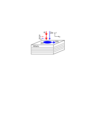
Figure 1: (Color online) A sketch of the optical current injection scenario. The MQW structure with $q=4$ (gray bands for GaAs) is shown. Vectors $\widehat{e}_{\omega(2\omega)}$ correspond to the polarization of the photons. The injected charge density follows the profiles of the $2\omega$-beam and the $square$ of the $\omega$-beam intensity, which are the same due to the $2\omega$ generation procedure (frequency doubling in nonlinear crystal). $U(0)$ is the initial macroscopic speed of the electron puddle.

To reduce the system of partial differential equations, we introduce a full basis set in the form of the harmonic oscillator wave functions

$$\Psi_{n_{1},n_{2}}\left(\mathbf{r}\right)=\psi_{n_{1}}(x)\psi_{n_{2}}(y),\qquad\psi_{n}(x)=\frac{H_{n}\left(x/\Lambda\right)}{\pi^{1/4}\sqrt{n!2^{n}}}e^{-x^{2}/2\Lambda^{2}},$$ (3)

where $H_{n}\left(x/\Lambda\right)$ is the Hermite polynomial of the $n-$th order. The key point of our approach is the expansion of the possible solutions in a finite basis in the form:

$$N_{e}=\sum_{n_{1},n_{2}}^{n_{\max}}N_{n_{1},n_{2}}^{e}(t)\Psi_{n_{1},n_{2}}\left(\mathbf{r}\right);\qquad u_{i}=\sum_{n_{1},n_{2}}^{n_{\max}}u_{n_{1},n_{2}}^{(i)}(t)\Psi_{n_{1},n_{2}}\left(\mathbf{r}\right)+U_{i}\left(t\right).$$ (4)

Here $i=x,y$ is the Cartesian index. To improve the convergence, we include a known function of time $U_{i}\left(t\right)$ in the right-hand side of Eq.(4). This function is obtained by solving the linear equations of motion in the rigid spot approximation Sherman06 . In the geometry considered here, $U_{y}\left(t\right)=0$, and, therefore, we drop the Cartesian index of $U_{x}\left(t\right)$. The electric fields at the point $\mathbf{r}$ are

$$\mathbf{E}^{e,h}\left(\mathbf{r},t\right)=\mp\frac{e}{\varepsilon}\sum_{n_{1},n_{2}}^{n_{\mathrm{max}}}N_{n_{1},n_{2}}^{e,h}(t)\int\Psi_{n_{1},n_{2}}\left(\widetilde{\mathbf{r}}\right)\frac{\mathbf{r}-\widetilde{\mathbf{r}}}{\left|\mathbf{r}-\widetilde{\mathbf{r}}\right|^{3}}d^{2}\widetilde{r},$$ (5)

where the upper (lower) sign corresponds to electrons (holes). If a QW is located close to the semiconductor-air interface, the role of the image charges which can be taken into account with the Green function technique Sipe81 , increases the field by a factor of two. Since $\Lambda$ is typically much larger than the distance between the QWs, within our assumption that the excitation of all the wells is the same, the electric field at a point $\mathbf{r}$ in each well and the subsequent dynamics is the same.

The state and the motion of the electron spot is then fully described by a $3\times\left(n_{\max}+1\right)^{2}-$component vector $S_{\alpha},$ where $\alpha$ is a two-component index corresponding to indices $n_{1}$ and $n_{2}.$ By projecting the equations (1),(2) and (5) on the set of $\Psi_{n_{1},n_{2}}\left(\mathbf{r}\right)$, we obtain the system of ordinary nonlinear differential equations in the form

$$\frac{dS_{\alpha}}{dt}=\sum_{\eta,\mu}\mathcal{C}\left(\alpha;\eta,\mu\right)S_{\eta}S_{\mu}-\sum_{\zeta}{\Gamma}\left(\alpha;\zeta\right)S_{\zeta}.$$ (6)

Here the matrix $\mathcal{C}\left(\alpha;\eta,\mu\right)$ is determined by the spatial dependence of concentration and velocity, and the electron-hole drag, while the matrix ${\Gamma}\left(\alpha;\zeta\right)$ depends on the Coulomb forces and momentum relaxation times. The full matrices will be presented elsewhere.

The initial conditions are given by: (i) $N_{0,0}^{e}(0)=\sqrt{\pi}N_{0},\;N_{n_{1},n_{2}}^{e}(0)=0$ (if $n_{1}>0$ or $n_{2}>0$), and (ii) $u_{n_{1},n_{2}}^{(i)e}(0)=0.$ Conditions (i) correspond to the initial injection of density in the Gaussian mode $\Psi_{0,0}\left(\mathbf{r}\right)$ only. Due to the symmetry of the problem $N_{n_{1},2m+1}^{e}(t)$, $u_{n_{1},2m+1}^{(x)}(t)$ and $u_{n_{1},2m}^{(y)}(t)$ will remain zero. The initial speed of the electron spot $U(0)$ is determined Bhat00 by the photon excess energy and $\Delta\phi$.

At very short times after the injection the carriers propagate ballistically, and then the motion becomes diffusive and influenced by the Coulomb forces. A simple characterization of the motion of the charge is given by the first moment of the concentration,

$$\left\langle x(t)\right\rangle=\frac{1}{N_{\rm t}}{\int xN_{e}\left(\mathbf{r},t\right)d^{2}r},\quad N_{\mathrm{t}}=\pi N_{0}\Lambda^{2},$$ (7)

where $N_{\mathrm{t}}$ is the total number of injected electrons. The relaxation and Coulomb interaction guarantee that $\xi\equiv\left\langle x(t)\right\rangle/\Lambda$ is always small in our systems. Were the rigid spot approximation valid, the amplitude of the nonzero higher terms $N_{n,0}^{e}$ would drop off as $\xi^{n}$. The main qualitative result of our investigations is that this is often not so for reasonable excitation parameters. Instead, the concentration-dependent Coulomb forces and drag lead to a deformation of the spot and, therefore, to an increase in the number of $\Psi_{n_{1},n_{2}}$ terms with non-negligible amplitude in the sums, and to a complicated spot structure. In the course of time, a few of the $N_{n_{1},n_{2}}^{e}(t)$ components can become of the same order of magnitude, although all small compared to $N_{0,0}(0)$ due to a relatively small spot displacement $\xi\ll 1$. The number of higher terms that are important depends mainly on the structure of the $\mathcal{C}\left(\alpha;\eta,\mu\right)$-matrix, with their relative contribution dependent on the parameters $\tau_{e}\Omega_{\mathrm{pl}}$ and $\tau_{e}/\tau_{eh}$. In contrast to the scattering by phonons and disorder, which stabilizes the spot motion and does not lead to its distortion, the role of electron-hole collisions is two-fold. On one hand, it stops the motion of the spot as a whole, on the other hand, it generates higher components in the velocity pattern due to nonuniform velocity evolution. The nonuniform velocity distribution produced by the Coulomb forces and the drag then leads to a nonuniform density distribution due to continuity. So the joint effects of the Coulomb forces and the drag lead to a ”buckling” of the electron spot along the direction of its velocity. The buckling becomes more pronounced as the space-charge effects, characterized by the parameter $\tau_{e}\Omega_{\mathrm{pl}}$, increase.

Figure 2: (Color online) The change in the electron density distribution compared to the injected density at $t=80$ fs (left column) and $t=1.5$ ps (right column). The MQW parameters are $q=1$ (upper row) and $q=16$ (second row). Relaxation times are $\tau_{e}=80$ fs, $\tau_{eh}$ = 150 fs. The spot size $\Lambda=1$ $\mu$m, $N_{s}=$10¹¹ cm${}^{-2},$ $U(0)=400$ km/s.

This is illustrated in Fig.2, where we show the pattern of the change in the electron density at two times, for samples with $q=1$ and $q=16$ buried deep within bulk Al_xGa_1-xAs where Eq.(5) is applicable. On the time scales of the ballistic regime, $t\leq\tau_{e},$ in both samples the spot moves as a rigid distribution with

$$N_{e}=N_{0}\exp\left[-\left(x-\left\langle x(t)\right\rangle\right)^{2}/2\Lambda^{2}\right]\exp\left[-y^{2}/2\Lambda^{2}\right],$$ (8)

and the corresponding density component develops as $N_{1,0}^{e}(t)=N_{0,0}^{e}(0)\xi/\sqrt{2}$. This is clearly seen in the left column of the Fig. 2, where the density profile is almost the same for systems with weak ($q=1$) and much stronger ($q=16$) space-charge effects at $t=80$ fs, and is well described by Eq.(8). At 1.5 ps, the profile for the $q=1$ system buckles only slightly; a ”rigid spot” picture is applicable. But for $q=16$ the behavior at these times is much more complicated, with several $\Psi_{n_{1},n_{2}}$ states contributing, and the profile changing from oval to bow-shaped. Here the ”rigid spot” approximation is no longer reasonable, and a more general ”distorted puddle” picture emerges. More insight can be obtained from the current density $N_{e}(\mathbf{r})u_{x}(\mathbf{r})$ distribution in Fig.3. At $t=80$ fs the patterns for $q=1$ and $q=16$ look similar. At $t=160$ fs, the distributions already differ very considerably, and the pattern for $q=16$ is much more nonuniform than that for $q=1$.

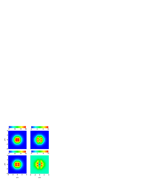
Figure 3: (Color online) The electron current density distribution (in arb. units) at $t=80$ fs (left column) and $t=160$ fs (right column). The MQW parameters are $q=1$ (upper row) and $q=16$ (second row). Other parameters are the same as in Fig. 2

It is interesting to see the effect of the real spot shape on gross features of the density distribution, such as its first moment (7). We evaluate this from our calculations as

$$\left\langle x(t)\right\rangle=\sum_{n_{1}=1}^{n_{\lim}}\sum_{n_{2}=0}^{n_{\max}}\frac{N_{n_{1},n_{2}}^{e}(t)}{N_{\mathrm{t}}}\int x\psi_{n_{1}}\left(x\right)dx\int\psi_{n_{2}}\left(y\right)dy,$$ (9)

and present in Fig.4 the results for $q=4$ and $q=16$ samples. The upper limit $n_{\lim}$ here is less than the number of Hermite-Gaussian states in the basis $n_{\max}$, since the contributions of the upper states cannot be calculated with a high precision; this problem is typical for calculations with finite basis. Sherman06a For this set of parameters we find that $n_{\max}=14$ and $n_{\lim}=7$ give converged results. In addition, Fig.4 shows the displacement in the rigid spot approximation Sherman06 , where the dynamics yields $\left\langle x_{\mathrm{rsa}}(t)\right\rangle=U(0)e^{-\gamma t}\mathrm{sinh}\left({\gamma}_{\rm pl}t\right)/{\gamma}_{\rm pl}$ with $2\gamma=1/\tau_{e}+1/2\tau_{eh}$, ${\gamma}_{\rm pl}^{2}=\gamma^{2}-\Omega_{\mathrm{pl}}^{2}$. With the stronger space-charge effects that arise for a larger number of wells, the deviation from the rigid spot approximation becomes more severe. However, both $\left\langle x_{\mathrm{rsa}}(t)\right\rangle$ and $\left\langle x(t)\right\rangle$ reach their maxima at almost the same time $t_{0}=2\tau_{e}\left|\ln(\Omega_{\mathrm{pl}}\tau_{e})\right|$, and the maximum values are very close to each other. The difference begins developing at $t>t_{0}$, when the buckling effects become more pronounced. The curves for small value of $\tau_{eh}=50$ fs show that a decrease in $\tau_{eh}$ does not qualitatively modify the dynamics in our range of parameters. However, in a regime with $\tau_{eh}\ll\tau_{e}$ a decrease in $\tau_{eh}$ can lead to an increase in the puddle distortion. We turn to the influence of this distortion on experimental results in a separate publication.

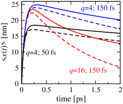
Figure 4: (Color online) Mean spot displacement $\left\langle x(t)\right\rangle$ (solid lines) and $\left\langle x_{\rm rsa}(t)\right\rangle$ (dashed lines). Parameters $q$ and $\tau_{eh}$ are marked near the lines. Other parameters are the same as in Fig. 2.

To conclude, we have shown that within a hydrodynamic model a Hermite-Gaussian expansion can be used to study the dynamics of currents injected optically by coherent control in MQW samples. As samples with increasing numbers of QWs are considered, we find the resulting dynamics shows a complicated buckling behavior in the density distribution that is driven by space-charge effects, with the charge density departing more and more from what a rigid spot approximation would predict. The details of our calculated results reflect both the simple dynamics (1),(2) we adopt, and the assumption of equal excitation of all the quantum wells. But it is unlikely that a relaxation of these approximations, and the richer dynamics that would result, would lead to a more rigid behavior of the charge puddle.

For $\tau_{eh}=150$ fs, we find that the complex behavior, associated with a number of comparable Hermite-Gaussian amplitudes, emerges at $\Omega_{\rm pl}\tau_{e}\approx 0.1$, well within the overdamped regime, and is determined by this parameter rather than by the electron-hole separation. How sensitive various experimental probes will be to this deviation from rigid spot dynamics has yet to be examined; at least it has significant consequences on the evolution of the first moment of density on the timescale of a picosecond.

Our numerical consideration relies on the finite basis analysis. In the overdamped regime we have considered here a fast decay of the off-diagonal Coulomb matrix elements with the distance between the states ensures the applicability of relatively small basis sets. As we consider systems with stronger Coulomb interaction, the basis should be extended. We can naturally expect the distortion of the carrier puddles to get more pronounced, and an interesting problem is whether it can lead to a chaotic behavior Pershin07 when many Hermite-Gaussian terms form the density and velocity patterns.

We are grateful to H. van Driel, J. McLeod, A. Najmaie, I. Rumyantsev, and A.L. Smirl for numerous valuable discussions. This work was supported by the Natural Sciences and Engineering Research Council of Canada (NSERC).

References

- (1) Nonequlibrium Carrier Dynamics in Semiconductors (M. Saraniti and U. Ravaioli, Eds.), Springer (2006)
- (2) S. Saikin, Yu. V. Pershin, and V. Privman, IEEE Proc. Circuits Devices Syst. 152, 366 (2005), Y. V. Pershin, Phys. Rev. B 75, 165320 (2007)
- (3) M. Q. Weng, M. W. Wu, and L. Jiang, Phys. Rev. B 69, 245320 (2004), J. Zhou, J. L. Cheng, and M. W. Wu, Phys. Rev. B 75, 045305 (2007)
- (4) H. T. Duc, Q. T. Vu, T. Meier, H. Haug, and S. W. Koch, Phys. Rev. B 74, 165328 (2006), H. T. Duc, T. Meier, and S. W. Koch, Phys. Rev. Lett. 95, 086606 (2005)
- (5) I. Rumyantsev, A. Najmaie, R.D.R. Bhat, and J.E. Sipe, International Quantum Electronics Conference, IEEE, Pascataway, NJ, 2004, p. 486.
- (6) J. Wühr, V. M. Axt, and T. Kuhn, Phys. Rev. B 70, 155203 (2004), M. Glanemann, V. M. Axt, and T. Kuhn, Phys. Rev. B 72, 045354 (2005)
- (7) R. D. R. Bhat and J. E. Sipe, Phys. Rev. Lett. 85, 5432 (2000), Ali Najmaie, R.D.R. Bhat, and J. E. Sipe, Phys. Rev. B 68, 165348 (2003)
- (8) M. J. Stevens, A. Najmaie, R. D. R. Bhat, J. E. Sipe, and H. M. van Driel, and A.L. Smirl, J. Appl. Phys. 94, 4999 (2003), M. J. Stevens, A. L. Smirl, R. D. R. Bhat, A. Najmaie, J. E. Sipe, and H. M. van Driel, Phys. Rev. Lett. 90, 136603 (2003)
- (9) J. Hübner, W.W. Rühle, M. Klude, D. Hommel, R.D.R. Bhat, J.E. Sipe, and H.M van Driel, Phys. Rev. Lett. 90, 216601 (2003).
- (10) E.Ya. Sherman, Ali Najmaie, H.M. van Driel, Arthur L. Smirl and J.E. Sipe, Solid State Comm. 139, 439 (2006)
- (11) L. L. Bonilla and H. T. Grahn, Rep. Prog. Phys. 68, 577 (2005)
- (12) R.A. Hopfel, J. Shah, P.A. Wolff, and A.C. Gossard, Phys. Rev. Lett. 56, 2376 (1986), R.A. Hopfel, J. Shah, P.A. Wolff, and A.C. Gossard, Appl. Phys. Lett. 49, 573 (1986)
- (13) H. Zhao, A.L. Smirl and H.M. van Driel, Phys. Rev. B 75, 075305 (2007), J.-Y. Bigot, M. T. Portella, R. W. Schoenlein, J. E. Cunningham, and C. V. Shank, Phys. Rev. Lett. 67, 636 (1991), W. A. Hügel, M. F. Heinrich, and M. Wegener, Phys. Status Solidi B 221, 473 (2000).
- (14) J.E. Sipe, Surface Science 105, 489 (1981), J.E. Sipe, Journal of the Optical Society of America B 4, 481 (1987)
- (15) C. Weber, F. Banit, S. Butscher, A. Knorr, and A. Wacker, Appl. Phys. Lett. 89, 091112 (2006)
- (16) E. Ya. Sherman and J. E. Sipe, Phys. Rev. B 73, 205335 (2006)
- (17) N. Bushong, Yu. V. Pershin, M. Di Ventra, Phys. Rev. Lett. 99, 226802 (2007)