Photon emission by an atom in a lossy cavity

Abstract

The dynamics of an initially excited two-level atom in a lossy cavity is studied by using the quantum trajectory method. Unwanted losses are included, such as photon absorption and scattering by the cavity mirrors and spontaneous emission of the atom. Based on the obtained analytical solutions, it is shown that the shape of the extracted spatiotemporal radiation mode sensitively depends on the atom-field interaction. In the case of a short-term atom-field interaction we show how different pulse shapes for the field extracted from the cavity can be controlled by the interaction time.

I Introduction

A single atom interacting with a quantized radiation-field mode in a high-$Q$ optical cavity plays an important role in quantum optics not only due to its conceptual relevance, but also because it appears as a basic element in various schemes, such as in the field of quantum information science (for a review see, e.g., Refs. HarocheRaimond ; Walther1 ; Walther2 ; Nielsen ). Cavity quantum electrodynamics (QED) has been used for the generation and processing of nonclassical radiation, as, for example, in the single-atom maser Haroche:347 ; Gallas:414 ; Meschede:551 ; Rempe:353 ; Brune:1899 or in the optical domain Thompson:1132 . The quantum control of single-photon emission from an atom in a cavity for generating single-photon Fock states on demand has been realized Monroe:238 , and single-photon Fock state generation of high efficiency has been a key requirement in various applications such as quantum cryptography Bennett:2724 ; Luetkenhaus:52304 or quantum networking for distribution and processing of quantum information Cirac:3221 ; Knill:46 . Recently, single-photon sources operating on the basis of adiabatic passage with just one atom trapped in a high-$Q$ optical cavity have been realized Parkins:3095 ; Hennrich:4872 ; Mckeever:1992 ; Hijlkema:253 . In this way, the generation of single photons of known circular polarization has been possible Wilk:063601 . Moreover, the adjustment of the spatiotemporal profile of single-photon pulses has been achieved Kuhn:067901 ; Keller:1075 .

In view of the widespread applications of cavity-assisted single-photon sources, it is of great importance to carefully study the quantum state of the field escaping from a cavity. Let us consider the simplest case of a two-level atom that near-resonantly interacts with a narrow-band cavity-field mode. On a time scale that is sufficiently short compared to the inverse bandwidth of the mode, the radiative and non-radiative cavity losses may be disregarded, and the atom-field dynamics can be described by the familiar Jaynes-Cummings model Jaynes:89 . Clearly, for longer times, the atom-cavity system can no longer be regarded as being a closed system, and the losses must be taken into account. Since the wanted outgoing field represents, from the point of view of the atom–cavity system, radiative losses, the study of the input–output problem necessarily requires inclusion in the theory of the effects of losses. Such a system, consisting of a two-level atom interacting with a single mode of a lossy cavity, has been widely considered in the past decades. Some of the initial theoretical works treating the effects of losses on the Jaynes-Cummings dynamics can be found in Refs. Barnett:2444 ; Filipowicz:3077 ; Puri:3433 ; Kuklinski:3175 ; Risken:346 ; Cirac:4541 ; Quang:6092 ; Alsing:13 ; Banacloche:2221 . For a review on this topic see, e.g., Refs. Shore:1195 ; Barnett:2033 . Anyway, a detailed characterization of the cavity output field in such a system still presents some open questions of significant interest, as, for example, the control of the pulse shape of the emitted photon.

There are primarily two approaches to this problem, which are based on either quantum field theory or quantum noise theory. In quantum field theory, the system is commonly described on the basis of Maxwell’s equations as used in macroscopic QED Knoell:1 ; VogelWelsch . It has been shown that an approximate description of the fields inside and outside a cavity can be formulated in terms of quantum Langevin equations and input-output relations Knoell:543 ; Plank:1791 . Macroscopic QED can also be used to study effects of unwanted losses, such as scattering and absorption losses caused by the cavity mirrors Khanbekyan:053813 ; Semenov:033803 ; Semenov:013807 . More recently, the photon emission by an excited atom in a cavity has been analyzed by the method of macroscopic QED Khanbekyan:quant-ph . By using a source-quantity representation of the electromagnetic field, the properties of the outgoing field are investigated. In such an approach the field inside and outside the cavity is combined in a unique radiation mode, without regarding the fields inside and outside the cavity as representing independent degrees of freedom.

Conversely, in quantum noise theory the fields inside and outside a cavity are regarded as representing independent degrees of freedom Collett:1386 ; Gardiner:3761 ; GardinerZoller . Accordingly, such a theory is based on discrete and continuous mode expansions of the fields inside and outside the cavity, respectively. Thus the operators of the intracavity and external fields are regarded as commuting quantities. The continuum of the external modes is regarded as playing the role of a dissipative system. Its effect on the dynamics of the intracavity modes can be treated by quantum Langevin equations, or, alternatively, by master equations Haake ; Louisell ; Davies . For obtaining their solution one can apply, for example, the quantum trajectory method Dalibard:580 ; Dum:4382 ; Carmichael .

In the present paper we consider a two-level atom interacting with a lossy cavity, within the framework of quantum noise theory, giving particular emphasis to the derivation of the pulse shape of the emitted photon. The dynamical evolution of the open quantum system under study is described by a master equation for the reduced density operator of the atom-cavity system. The effects of unwanted losses, such as spontaneous emissions of the two-level atom out the side of the cavity and photon absorption and scattering by the cavity mirrors, are also taken into account. For an initially excited two-level atom in an empty cavity, we solve the master equation analytically by using the quantum trajectory method. In order to characterize the cavity output field, described by a single-photon spatiotemporal mode, we connect the probability to measure a photon in this mode with the photodetection probability as given by the quantum trajectory theory. This allows us to derive the shape of the mode of the extracted cavity field, which shows a clear mapping of the intracavity-field dynamics onto the mode of the output field. Moreover, the probability of the outgoing mode to carry a single-photon Fock state is calculated. After considering the case of a continuing atom-field interaction, we also analyze the short-term atom-field interaction. It is shown that, by changing the interaction time of the atom with the cavity, the mode structure of the outgoing field results in different pulse shapes of the single-photon wave packet. This opens possibilities to control the shape of the pulse.

The paper is organized as follows. In Sec. II the master equation describing the dynamics of the atom-cavity system is introduced, and the problem is solved analytically by using the quantum trajectory method. In Sec. III, giving a description of the single-photon wave packet in terms of spatiotemporal mode functions, the shape of the mode of the extracted cavity field is obtained. In Sec. IV we analyze short-term atom-field interactions and obtain different shapes of the mode of the extracted field. A summary and some concluding remarks are given in Sec. V.

II Damped atom-field dynamics

In this section we analyze the dynamics of the system under scrutiny starting from a master equation and solving it by using the quantum trajectory theory. We consider a single two-level atomic transition of frequency $\omega_{a}$ coupled to a cavity mode of frequency $\omega_{c}$. The cavity mode is detuned by $\Delta$ from the two-level atomic transition frequency, $\omega_{\rm a}=\omega_{\rm c}+\Delta$, and is damped by losses through the partially transmitting cavity mirrors, cf. Fig. 1. In addition to the wanted outcoupling of the field, the photon can be spontaneously emitted out the side of the cavity into modes other than the one which is preferentially coupled to the resonator. Moreover, the photon may be absorbed or scattered by the cavity mirrors.

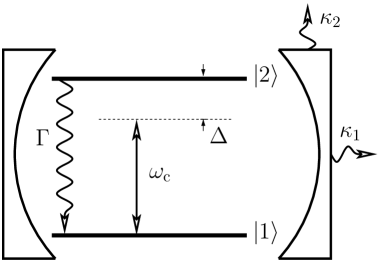
Figure 1: The cavity mode of frequency $\omega_{\rm c}$ is detuned by $\Delta$ from the two-level atomic transition frequency $\omega_{\rm a}=\omega_{\rm c}+\Delta$. $\kappa_{1}$ and $\kappa_{2}$ are the photon escape rate of the cavity and the cavity mirrors’ absorption and scattering rate, respectively. $\Gamma$ is the dipole relaxation rate from level $|2\rangle$ to $|1\rangle$.

Treating the dissipation due to the cavity losses in a standard way Haake ; Louisell ; Davies , the dynamical evolution of the reduced density operator $\hat{\rho}(t)$ of the atom and the cavity field is described by the following master equation

$$\frac{d\hat{\rho}(t)}{dt}\!\!\! = \!\!\!\frac{1}{i\hbar}\!\left[\hat{H},\hat{\rho}(t)\right]\!+\!\sum_{i=1}^{2}\frac{\kappa_{i}}{2}\!\left[2\hat{a}\hat{\rho}(t)\hat{a}^{\dagger}\!-\!\hat{a}^{\dagger}\hat{a}\hat{\rho}(t)\!-\!\hat{\rho}(t)\hat{a}^{\dagger}\hat{a}\right]$$ (1)

$$+ \frac{\Gamma}{2}\left[2\hat{A}_{12}\hat{\rho}(t)\hat{A}_{21}-\hat{A}_{22}\hat{\rho}(t)-\hat{\rho}(t)\hat{A}_{22}\right].$$

Here $\kappa_{1}$ and $\kappa_{2}$ are the photon escape rate of the cavity and the cavity mirrors’ absorption and scattering rate, respectively. We denote by $\Gamma$ the spontaneous emission rate of the two-level atom. The Hamiltonian that describes the atom-cavity interaction is given, in the rotating-wave approximation, by

$$\hat{H}=\hbar{g}\left(\hat{a}\hat{A}_{21}+\hat{a}^{\dagger}\hat{A}_{12}\right)+\hbar\Delta{\hat{A}}_{22}\,,$$ (2)

where $\hat{a}$ and $\hat{a}^{\dagger}$ are annihilation and creation operators for the cavity field, respectively, and $\hat{A}_{ij}=|i\rangle\langle j|$ ($i,j=1,2$), where $|1\rangle$ and $|2\rangle$ are the two atomic energy eigenstates. Moreover, $g$ is the atom-cavity coupling constant. Here we are considering an interaction picture with respect to $\hat{H}_{0}-\hbar\Delta{\hat{A}}_{22}$, where ${\hat{H}}_{0}=\hbar\omega_{\rm c}\hat{a}^{\dagger}\hat{a}+(1/2)\hbar\omega_{\rm a}({\hat{A}}_{22}-{\hat{A}}_{11})$.

For notational convenience, in the following we will identify the state $|a\rangle$ with the state $|2,0\rangle$, the atom in the upper level, and no photon in the cavity. The state $|a\rangle$ will be considered to be the initial state of the system. Moreover, we will indicate with $|b\rangle$ the state $|1,1\rangle$, the atom in the lower level, and one photon in the cavity. Due to photon extraction through the cavity mirror, photon absorptions, or spontaneous emissions, the quantum state of the atom-cavity system is projected into the state $|c\rangle$, that indicates the state $|1,0\rangle$, i.e., the atom in the lower level and no photon in the cavity. It follows that the Hilbert space that describes the atom-cavity system under scrutiny is, in this model, simply spanned by the three vectors $|a\rangle$, $|b\rangle$ and $|c\rangle$.

To evaluate the time evolution of the system different approaches can be used, see, for example, Refs. Agarwal:1757 ; Puri:3610 ; Briegel:3311 . Here we have found it quite convenient to use a quantum trajectory approach Dalibard:580 ; Dum:4382 ; Carmichael to obtain our analytical solutions. In this approach the dynamical evolution of the unnormalized state vector $|\bar{\psi}(t)\rangle$, that describes the system at time $t$, is governed by a nonunitary Schrödinger equation with a non-Hermitian Hamiltonian. The evolution generated by this Schrödinger equation is randomly interrupted, from time to time, by the action of collapse, or jump, operators.

More precisely, in our specific case, considering the system prepared at time $t_{0}=0$ in the state $|a\rangle$, to determine the state vector of the system at a later time $t$, assuming that no jump has occurred between time $t_{0}$ and $t$, we have to solve the nonunitary Schrödinger equation

$$i\hbar\frac{d}{dt}|\bar{\psi}_{\rm no}(t)\rangle=\hat{H^{{}^{\prime}}}\,|\bar{\psi}_{\rm no}(t)\rangle\,,$$ (3)

where $\hat{H^{{}^{\prime}}}$ is the non-Hermitian Hamiltonian given by

$$\hat{H^{{}^{\prime}}}=\hat{H}-i\hbar\frac{\kappa}{2}\hat{a}^{\dagger}\hat{a}-i\hbar\frac{\Gamma}{2}\hat{A}_{22}\,,$$ (4)

with $\hat{H}$ given by Eq. (2), and where we have defined

$$\kappa=\kappa_{1}+\kappa_{2}\,.$$ (5)

If no jump has occurred between time $t_{0}$ and $t$, the system evolves via Eq. (3) in the unnormalized state

$$|\bar{\psi}_{\rm no}(t)\rangle=\alpha(t)|a\rangle+\beta(t)|b\rangle\,.$$ (6)

In this case the conditioned density operator for the atom-cavity system is given by

$$\hat{\rho}_{\rm no}(t) = \frac{|\bar{\psi}_{\rm no}(t)\rangle\langle\bar{\psi}_{\rm no}(t)|}{\langle\bar{\psi}_{\rm no}(t)|\bar{\psi}_{\rm no}(t)\rangle}\,.$$ (7)

Here we have used the word conditioned to stress the fact that this is the density operator at time $t$ one obtains conditioned to the fact that no jump has occurred between time $t_{0}$ and $t$.

The evolution governed by the nonunitary Schrödinger equation (3) is randomly interrupted by three kinds of jumps, $\hat{J}_{1}$, $\hat{J}_{2}$ and $\hat{J}_{\rm s}$ given by

$$\hat{J}_{i}=\sqrt{\kappa_{i}}\hat{a}~{}~{}~{}(i=1,2)\,,$$ (8)

$$\hat{J}_{\rm s}=\sqrt{\Gamma}\,\hat{A}_{12}\,.$$ (9)

The jump operators $\hat{J}_{1}$ and $\hat{J}_{2}$ are related to a photon extracted from the cavity and a photon absorbed or scattered by the mirrors, respectively. The jump operator $\hat{J}_{\rm s}$ is related to a photon spontaneously emitted by the atom. If a jump has occurred at time $t_{\rm J}$, $t_{\rm J}\in(t_{0},t]$, the wavevector is found collapsed in the state $|c\rangle$ due to the action of one of the jump operators

$$\hat{J}_{i}\,|\bar{\psi}_{\rm no}(t_{\rm J})\rangle\!=\!\sqrt{\kappa_{i}}\,\hat{a}|\bar{\psi}_{\rm no}(t_{\rm J})\rangle\rightarrow|c\rangle~{}~{}(i=1,2),$$ (10)

$$\hat{J}_{\rm s}\,|\bar{\psi}_{\rm no}(t_{\rm J})\rangle\!=\!\sqrt{\Gamma}\,\hat{A}_{12}|\bar{\psi}_{\rm no}(t_{\rm J})\rangle\rightarrow|c\rangle\,.$$ (11)

It is clear that in the problem under study we can have only one jump. Once the system collapses in the state $|c\rangle$ the nonunitary Schrödinger equation (3) simply keeps it there forever. In this case the conditioned density operator at time $t$ is given by

$$\hat{\rho}_{\rm yes}(t)=|c\rangle\langle c|\,,$$ (12)

where we indicate with “yes” the fact that a jump has occurred.

According to the quantum trajectory method, the density operator $\hat{\rho}(t)$ is obtained by performing an ensemble average over the different conditioned density operators at time $t$. In the present case, starting at time $t_{0}$ with the density operator $\hat{\rho}_{0}=|a\rangle\langle a|$, the ensemble average is performed over the two possible realizations (histories) “yes” and “no”:

$$\hat{\rho}(t)=p_{\rm no}(t)\hat{\rho}_{\rm no}(t)+p_{\rm yes}(t)\hat{\rho}_{\rm yes}(t)\,.$$ (13)

Here $p_{\rm no}(t)$ and $p_{\rm yes}(t)$ are the probability that between the initial time $t_{0}$ and time $t$ no jump and one jump has occurred, respectively. Of course, $p_{\rm no}(t)+p_{\rm yes}(t)=1$. The density operator given by Eq. (13) tells us that the system at time $t$ is in a statistical mixture: either no photon has escaped from the cavity or one (and only one) photon has escaped.

To evaluate $p_{\rm no}(t)$ we use the method of the delay function Dum:4382 . This method tells us that the probability $p_{\rm no}(t)$ is given by the square of the norm of the unnormalized state vector:

$$p_{\rm no}(t)=\parallel|\bar{\psi}_{\rm no}(t)\rangle\!\parallel^{2}=\langle\bar{\psi}_{\rm no}(t)|\bar{\psi}_{\rm no}(t)\rangle=|\alpha(t)|^{2}+|\beta(t)|^{2}\,.$$ (14)

From Eqs. (13) and (14) one obtains for the density operator $\hat{\rho}(t)$ the expression

$$\hat{\rho}(t) = |\alpha(t)|^{2}|a\rangle\langle a|+|\beta(t)|^{2}|b\rangle\langle b|+\alpha(t)\beta^{*}(t)|a\rangle\langle b|$$ (15)

$$+ \alpha^{*}(t)\beta(t)|b\rangle\langle a|+|\gamma(t)|^{2}|c\rangle\langle c|\,,$$

where we have defined

$$|\gamma(t)|^{2}\equiv p_{\rm yes}(t)=1-\left[|\alpha(t)|^{2}+|\beta(t)|^{2}\right]\,.$$ (16)

The physical meaning of $|\alpha(t)|^{2}$, $|\beta(t)|^{2}$ and $|\gamma(t)|^{2}$ is clear. They represent the probability that at time $t$ the system can be found either in $|a\rangle$, $|b\rangle$, or $|c\rangle$. Moreover, from the master equation (1), together with Eq. (15), one obtains

$$\frac{d|\gamma(t)|^{2}}{dt}={\rm Tr}\left[\frac{d\hat{\rho}(t)}{dt}|c\rangle\langle c|\right]=\kappa|\beta(t)|^{2}+\Gamma|\alpha(t)|^{2}\,.$$ (17)

To better understand the meaning of Eq. (17), it is useful to do the following consideration. According to the quantum trajectory theory, the probability for a jump, cf. Eqs. (8) and (9), to occur in the time interval $(t,t+dt]$ is given by $(i=1,2)$

$$p_{\rm i}(t)\!=\!\langle\hat{J}_{i}^{\dagger}\hat{J}_{i}\rangle_{t}\,dt=\kappa_{i}\,{\rm Tr}\left[\hat{\rho}(t)\hat{a}^{\dagger}\hat{a}\right]dt=\kappa_{i}|\beta(t)|^{2}dt$$ (18)

and

$$p_{\rm s}(t)\!=\!\langle\hat{J}_{\rm s}^{\dagger}\hat{J}_{\rm s}\rangle_{t}\,dt=\Gamma\,{\rm Tr}\left[\hat{\rho}(t)\hat{A}_{22}\right]\!dt\!=\!\Gamma|\alpha(t)|^{2}dt\,.$$ (19)

Of course, the increment in the time interval $dt$ for $p_{\rm yes}(t)$ is equal to $p_{1}(t)+p_{2}(t)+p_{\rm s}(t)$, so that we can write, using Eqs. (18), (19), and (16),

$$d|\gamma(t)|^{2}=dp_{\rm yes}(t)=\kappa|\beta(t)|^{2}dt+\Gamma|\alpha(t)|^{2}dt\,,$$ (20)

that is again Eq. (17). The physical meaning of this relation is quite clear. When the system is in $|b\rangle$, i.e. with probability $|\beta(t)|^{2}$, we can have an emission of a photon from the cavity or an absorption or scattering by the cavity mirrors (controlled by the parameter $\kappa$). When the system is in $|a\rangle$, i.e. with probability $|\alpha(t)|^{2}$, we can have a photon spontaneously emitted by the atom (controlled by the parameter $\Gamma$). The related jumps operators project the system into $|c\rangle$, hence producing an increment of $|\gamma(t)|^{2}$. Moreover, by integrating equation (20) one gets

$$p_{\rm yes}(t)=|\gamma(t)|^{2}=p_{\rm ext}(t)+p_{\rm abs}(t)+p_{\rm spo}(t)\,,$$ (21)

where we have defined

$$p_{\rm ext}(t)=\kappa_{1}\int_{0}^{t}dt^{\prime}|\beta(t^{\prime})|^{2}\,,$$ (22)

$$p_{\rm abs}(t)=\kappa_{2}\int_{0}^{t}dt^{\prime}|\beta(t^{\prime})|^{2}\,,$$ (23)

and

$$p_{\rm spo}(t)=\Gamma\int_{0}^{t}dt^{\prime}|\alpha(t^{\prime})|^{2}\,.$$ (24)

The function $p_{\rm ext}(t)$ represents the probability that a photon is extracted from the cavity in the time interval $[0,t]$, and $p_{\rm abs}(t)$ the probability that a photon is absorbed or scattered by the mirrors in the same time interval. Finally, $p_{\rm spo}(t)$ represents the probability that a spontaneous emission has occurred in time interval $[0,t]$.

Note that from Eqs. (22), (23), and (24) it follows that $p_{\rm ext}(t)$, $p_{\rm abs}(t)$, and $p_{\rm spo}(t)$ have to be monotonically increasing functions: the longer one waits, the larger is the probability that a photon has leaked out of the cavity, or is absorbed or scattered by the mirrors, or a spontaneous emission has occurred. Moreover, if we wait long enough a photon is certain to be emitted in one of the three ways, so that $\lim_{t\to\infty}|\gamma(t)|^{2}=1$. In this case $p_{\rm ext}(t)$ does not reach asymptotically the value $1$, due to the presence of spontaneous emissions and mirror absorption or scattering. If we take the limit $t\to\infty$ of Eq. (21), we get

$$p_{\rm ext}(\infty)+p_{\rm abs}(\infty)+p_{\rm spo}(\infty)=1\,.$$ (25)

In order to determine $\alpha(t)$ and $\beta(t)$ we have to solve the nonunitary Schrödinger equation, cf. Eqs. (3) and (4). This brings us to consider the following linear system of differential equations,

$$\left\{\begin{array}[]{ll}\dot{\alpha}(t)=-i\left(\Delta-i\frac{\Gamma}{2}\right)\alpha(t)-ig\beta(t)\,,\\ \dot{\beta}(t)=-ig\alpha(t)-\frac{\kappa}{2}\beta(t)\,.\end{array}\right.$$ (26)

For the initial conditions $\alpha(0)\!=\!1$ and $\beta(0)\!=\!0$, and defining

$$\Omega\equiv\sqrt{\frac{\kappa^{2}}{4}-4g^{2}-i\kappa\left(\Delta-i\frac{\Gamma}{2}\right)-\left(\Delta-i\frac{\Gamma}{2}\right)^{2}}\,,$$ (27)

we can write the solutions as

$${\alpha}(t)\!=\!\left[\frac{\kappa/2-i(\Delta-i\Gamma/2)}{\Omega}\sinh\left(\frac{\Omega t}{2}\right)\right.$$

$$~{}~{}~{}~{}~{}~{}~{}~{}+\left.\cosh\left(\frac{\Omega t}{2}\right)\right]\!e^{-[(\kappa+\Gamma)/4+i\Delta/2]t},$$

$${\beta}(t)\!=\!-\frac{2ig}{\Omega}\sinh\left(\frac{\Omega t}{2}\right)e^{-[(\kappa+\Gamma)/4+i\Delta/2]t}\,.$$ (28)

Figure 2: The probabilities $|\alpha(t)|^{2}$ (dashed line), $|\beta(t)|^{2}$ (dotted line), $p_{\rm ext}(t)$ (full line), and $p_{\rm abs}(t)$, $p_{\rm spo}(t)$ (dot-dashed lines) are shown for $2g/\kappa=10$, $\Delta/\kappa=0.1$, $\kappa_{1}/\kappa=0.9$, and $\Gamma/\kappa=0.5$.

Using the solutions given in Eq. (28), one can plot the probabilities to find at time $t$ the system in $|a\rangle$ or in $|b\rangle$, i.e. $|\alpha(t)|^{2}$ and $|\beta(t)|^{2}$, respectively, as well as $p_{\rm ext}(t)$, $p_{\rm abs}(t)$ and $p_{\rm spo}(t)$, as given by Eqs. (22)–(24). In Fig. 2 we show these functions for the parameters $2g/\kappa=10$, $\Delta/\kappa=0.1$, $\kappa_{1}/\kappa=0.9$, and for the realistic choice of $\Gamma/\kappa=0.5$, cf. Ref. Miller:S551 . Note that for $t\to\infty$, $|\alpha(t)|^{2}\to 0$, $|\beta(t)|^{2}\to 0$, and $p_{\rm ext}(t)+p_{\rm abs}(t)+p_{\rm spo}(t)=|\gamma(t)|^{2}\to 1$, as it is expected from Eqs. (28) and (16).

Let us consider $\Delta\!=\!0$ and $g\gg\kappa,\Gamma$. From Eq. (28) one immediately obtains

$$|\alpha(t)|^{2}=\cos^{2}(gt)e^{-(\kappa+\Gamma)t/2}\,,$$

$$|\beta(t)|^{2}=\sin^{2}(gt)e^{-(\kappa+\Gamma)t/2}\,.$$ (29)

In this case the system undergoes damped Rabi oscillations between $|a\rangle$ and $|b\rangle$ with frequency $2g$. From Eq. (29) one easily obtains, using Eqs. (22)–(24),

$$p_{\rm ext}(t)\!=\!\kappa_{1}\!\int_{0}^{t}dt^{\prime}|\beta(t^{\prime})|^{2}\!=\!\frac{\kappa_{1}}{\kappa+\Gamma}\left(1\!-\!e^{-(\kappa+\Gamma)t/2}\right),$$ (30)

$$p_{\rm abs}(t)\!=\!\kappa_{2}\!\int_{0}^{t}dt^{\prime}|\beta(t^{\prime})|^{2}\!=\!\frac{\kappa_{2}}{\kappa+\Gamma}\left(1\!-\!e^{-(\kappa+\Gamma)t/2}\right),$$ (31)

and

$$p_{\rm spo}(t)\!=\!\Gamma\!\int_{0}^{t}dt^{\prime}|\alpha(t^{\prime})|^{2}\!=\!\frac{\Gamma}{\kappa+\Gamma}\left(1\!-\!e^{-(\kappa+\Gamma)t/2}\right)\,.$$ (32)

From Eq. (21) we then get

$$p_{\rm yes}(t)=|\gamma(t)|^{2}=1-e^{-(\kappa+\Gamma)t/2}\,,$$ (33)

that shows a simple exponential behavior. For $t\!\to\!\infty$ we have $p_{\rm ext}(t)\!\to\!\kappa_{1}/(\kappa+\Gamma)$, $p_{\rm abs}(t)\!\to\!\kappa_{2}/(\kappa+\Gamma)$, $p_{\rm spo}(t)\!\to\!\Gamma/(\kappa+\Gamma)$, and $|\gamma(t)|^{2}\!\to\!1$.

III Single-photon wave packet

The analysis performed here, using a quantum trajectory approach, is implicitly based on an unraveling of the master equation (1) for the case of direct photoelectric detection of the field emitted from the cavity Carmichael . In experiments one uses a large number of photodetections to recover the properties of the electromagnetic field, also in the case of single-photon sources, see, e. g., Refs. Kuhn:067901 ; Keller:1075 . Properties like wave packet duration or wave packet bandwidth are analyzed with an ensemble of photons and cannot be determined from a measurement on just a single photon. In this respect it is important to carefully describe the arrival of photons at the photodetector.

For this purpose it is convenient, following the approach of Blow:4102 ; Legero:797 ; Legero:253 , to choose spatiotemporal modes for characterizing the single-photon wave packet. A stream of single photons emitted one after the other can be described by a state vector $|1_{\xi_{i}}\rangle$, where

$$|1_{\xi_{i}}\rangle=\hat{c}_{\xi_{i}}^{\dagger}|0\rangle\,.$$ (34)

Here $\hat{c}_{\xi_{i}}^{\dagger}$ is the creation operator for photons of spatiotemporal mode $\xi_{i}(t)$ defined as

$$\hat{c}_{\xi_{i}}^{\dagger}=\int_{0}^{\infty}dt\,\xi_{i}(t)\hat{b}^{\dagger}(t)\,,$$ (35)

where $\xi_{i}(t)=0$ for $t<0$, and $\hat{b}^{\dagger}(t)$ is given by

$$\hat{b}^{\dagger}(t)=\frac{1}{\sqrt{2\pi}}\int d\omega\,b^{\dagger}(\omega)e^{i\omega t}\,,$$ (36)

that is, the Fourier transform of the operator $\hat{b}^{\dagger}(\omega)$, the creation operator of quanta of a monochromatic wave of frequency $\omega$ in free space. From the relation

$$\left[\hat{b}(\omega),\hat{b}^{\dagger}(\omega^{{}^{\prime}})\right]=\delta(\omega-\omega^{{}^{\prime}})\,,$$ (37)

and from Eq. (36), it follows that

$$\left[\hat{b}(t),\hat{b}^{\dagger}(t^{\prime})\right]=\delta(t-t^{\prime})\,.$$ (38)

Given that the photon is in the mode $\xi_{i}$, i.e. it is described by the normalized function $\xi_{i}(t)$, according to

$$\int_{0}^{\infty}dt\,|\xi_{i}(t)|^{2}=1\,,$$ (39)

it is possible to construct a complete orthonormal set $\{\xi_{j}(t)\}$ of functions where

$$\int dt\,\xi_{i}(t)\xi_{j}^{*}(t)=\delta_{ij}\,,$$ (40)

and

$$\sum_{i}\xi_{i}^{*}(t)\xi_{i}(t^{\prime})=\delta(t-t^{\prime})\,.$$ (41)

From Eqs. (38) and (40) it is immediate to show that

$$\left[\hat{c}_{\xi_{i}},\hat{c}_{\xi_{j}}^{\dagger}\right]=\delta_{ij}\,,$$ (42)

so that the operators defined by Eq. (35) using the complete set of orthonormal functions $\{\xi_{j}(t)\}$ represent a set of independent bosons, and $\hat{c}_{\xi_{i}}$ can be used to construct number states in the usual way,

$$|n_{\xi_{i}}\rangle=\frac{1}{\sqrt{n!}}\left[\hat{c}_{\xi_{i}}^{\dagger}\right]^{n}|0\rangle\,.$$ (43)

The spatiotemporal mode function ${\xi_{i}}(t)$ is composed of an amplitude envelope $\epsilon_{i}(t)$ and a phase $\phi_{i}(t)$,

$$\xi_{i}(t)=\epsilon_{i}(t)e^{i\phi_{i}(t)}\,.$$ (44)

According to Eq. (39), the normalization reads as

$$\int_{0}^{\infty}dt\,\epsilon^{2}_{i}(t)=1\,.$$ (45)

If we now define the flux operator in units of photons per unit time,

$$\hat{f}(t)=\hat{b}^{\dagger}(t)\hat{b}(t)\,,$$ (46)

using the inverse relation of Eq. (35), $\hat{b}(t)=\sum_{i}\xi_{i}(t)\hat{c}_{\xi_{i}}$, we can write Eq. (46) as

$$\hat{f}(t)=\sum_{i}\sum_{j}\xi_{i}^{*}(t)\xi_{j}(t)\hat{c}_{\xi_{i}}^{\dagger}\hat{c}_{\xi_{j}}\,.$$ (47)

When no extra losses, such as spontaneous emissions out the side of the cavity or mirrors’ absorption or scattering, are considered, the density operator of the cavity output field for a photon in the mode $\xi_{i}$ is, in the Heisenberg picture, $\hat{\rho}_{\rm out}=|1_{\xi_{i}}\rangle\langle 1_{\xi_{i}}|$, cf. Ref. Legero:253 . When extra losses are included, the density operator of the cavity output field is given by the statistical mixture

$$\hat{\rho}_{\rm out}=p_{\rm ext}(\infty)|1_{\xi_{i}}\rangle\langle 1_{\xi_{i}}|+\left[1-p_{\rm ext}(\infty)\right]|0\rangle\langle 0|\,.$$ (48)

Note that $1-p_{\rm ext}(\infty)=p_{\rm abs}(\infty)+p_{\rm spo}(\infty)$, consistently with the fact that the zero-field contribution is related to the spontaneous emissions out the side of the cavity or to mirrors’ absorption or scattering. The probability density distribution of measuring the photon at a given time $t$ is then

$$P_{\xi_{i}}(t)={\rm Tr}\left[\hat{\rho}_{\rm out}\hat{f}(t)\right]=p_{\rm ext}(\infty)\epsilon_{i}^{2}(t)\,.$$ (49)

Of course, integrating Eq. (49), and using Eq. (45) we have

$$P_{\rm tot}=\int_{0}^{\infty}\!dt\,P_{\xi_{i}}(t)=p_{\rm ext}(\infty)\int_{0}^{\infty}\!dt\,\epsilon_{i}^{2}(t)=p_{\rm ext}(\infty)\,,$$ (50)

as it is expected.

Let us consider a photon in the mode $\xi_{i}$, whose amplitude envelope $\epsilon_{i}(t)$ does not change significantly in the detection time resolution $T$. The response probability of the detector within a time interval $[t-T/2,t+T/2]$ is then, using Eq. (49), given by

$$P_{\rm D}(t)\!=\!\int_{t-T/2}^{t+T/2}\!\!\!dt^{\prime}P_{\xi i}(t^{\prime})\simeq p_{\rm ext}(\infty)\epsilon_{i}^{2}(t)\,T.$$ (51)

In the case of a detector of quantum efficiency $\eta$, Eq. (51) becomes

$$P_{\rm D}(t)=\eta\,p_{\rm ext}(\infty)\epsilon_{i}^{2}(t)\,T\,.$$ (52)

In a usual experiment a large number of photodetection events are accumulated to obtain $P_{\rm D}(t)$, and from these measurements one gets $\epsilon_{i}(t)$. This consideration is important because it tells us how one can obtain the amplitude envelope of the mode function within a quantum trajectory formalism. The probability to measure between time $t-T/2$ and $t+T/2$ a “click” at the detector is equal to the probability to have a jump $\hat{J}_{1}$ in the same time interval, so that using Eq. (18), we get, in the case of a detector of efficiency $\eta$,

$$P_{\rm D}(t)=\eta\kappa_{1}{\rm Tr}\left[\hat{\rho}(t)\hat{a}^{\dagger}\hat{a}\right]T=\eta\kappa_{1}|\beta(t)|^{2}T\,.$$ (53)

Comparing this with Eq. (52) we obtain

$$\epsilon_{i}(t)=\sqrt{\frac{\kappa_{1}}{p_{\rm ext}(\infty)}}|\beta(t)|\,.$$ (54)

Let us check if Eq. (45) is still fulfilled. Using Eq. (22) we obtain

$$\int_{0}^{\infty}\!dt\,\epsilon_{i}^{2}(t)=\frac{1}{p_{\rm ext}(\infty)}\lim_{t\rightarrow\infty}\kappa_{1}\!\int_{0}^{t}\!dt^{\prime}|\beta(t^{\prime})|^{2}=1\,.$$ (55)

Figure 3: Plot of the amplitude envelope $\epsilon_{i}(z,t)\sqrt{p_{\rm ext}(\infty)/\kappa_{1}}$ for the spatiotemporal mode of the cavity output field, with parameters $2g/\kappa=10$, $\Delta/\kappa=0.1$, $\kappa_{1}/\kappa=0.9$, $\Gamma/\kappa=0.5$, and $\kappa t=7$.

To obtain Eq. (54) we have assumed that the photodetector was positioned just outside the cavity, at $z=0$, so that this equation gives the amplitude envelope of the spatiotemporal mode function at $z=0$. Of course we could imagine to position the detector in an arbitrary position $z$ (with $z>0$). In this case, because outside the cavity the field is propagating at the speed of light $c$, the amplitude envelope $\epsilon_{i}(z,t)$ is related to the one at position $z=0$ via the retarded time $t-z/c$. More precisely,

$$\epsilon_{i}(z,t)\!=\!\left\{\begin{array}[]{ll}\!\epsilon_{i}(0,t\!-\!\frac{z}{c})\!=\!\sqrt{\frac{\kappa_{1}}{p_{\rm ext}(\infty)}}\,\left|\beta(t\!-\!\frac{z}{c})\right|&\mbox{~{}$t>\frac{z}{c}>0$}\\ \\ \!0&\mbox{~{}~{}~{}$t<\frac{z}{c}\,.$}\end{array}\right.$$ (56)

Note that $|\beta(t)|^{2}$ represents the probability to find at time $t$ a photon inside the cavity. In this respect, Eq. (56) shows that the intracavity field dynamics determines the structure of the spatiotemporal mode of the output field. Moreover, in order to clarify the connection between $\epsilon_{i}(z,t)$ and the probability to emit a photon, it is useful to consider the following equation, obtained from Eqs. (56) and (22):

$$\int_{z/c}^{t}dt^{\prime}\,\epsilon_{i}^{2}(z,t^{\prime})=\frac{p_{\rm ext}(t-z/c)}{p_{\rm ext}(\infty)}~{}~{}~{}(t>z/c)\,,$$ (57)

where $p_{\rm ext}(t)$ represents the probability that a photon has leaked out of the cavity in the time interval $[0,t]$. Using Eq. (56) and the solution given by Eq. (28), in Fig. 3 we plot the amplitude envelope $\epsilon_{i}(z,t)\sqrt{p_{\rm ext}(\infty)/\kappa_{1}}$ for the spatiotemporal mode of the cavity output field for the case where the parameters $g$ and $\kappa$ are chosen as $2g/\kappa=10$, $\Delta/\kappa=0.1$, $\Gamma/\kappa=0.5$, and $\kappa t=7$. It is clearly seen that the intracavity dynamics strongly modulates the mode structure of the photon wave packet propagating outside the cavity.

IV Time control of the photon wave packet

Let us now consider the case where the interaction of the atom with the cavity-assisted field has a limited duration, so that it effectively terminates at time $\tau$. To analyze this situation we have obviously to split the dynamical evolution of the system in two distinct time intervals, one interval from the initial time $t_{0}=0$ to the time $\tau$, and the second interval for times $t$ greater than $\tau$. For times $t$ such that $0\leq t\leq\tau$, the evolution is still described by the one previously analyzed in Sec. II, with solutions given by Eq. (28). For times $t$ with $t>\tau$, when the interaction of the atom with the cavity is set to zero, the Hilbert space of the system (cavity field) reduces to that spanned by the two Fock-state vectors $|1\rangle$ and $|0\rangle$ of the cavity field. At time $\tau$ the cavity field, obtained by tracing over the atomic states in Eq. (15), is described by the following density operator:

$$\hat{\rho}(\tau)=\left[1-|\beta(\tau)|^{2}\right]|0\rangle\langle 0|+|\beta(\tau)|^{2}|1\rangle\langle 1|\,,$$ (58)

where $\beta(\tau)$ is given by Eq. (28).

To analyze the dynamical evolution, for $t>\tau$, of this initial state, we follow the procedure given by the quantum trajectory theory when the initial state is not a pure state, but a statistical mixture Dalibard:580 ; Dum:4382 ; Carmichael . For the part related to $\left[1-|\beta(\tau)|^{2}\right]|0\rangle\langle 0|$, one has to start with the state vector $|\psi(\tau)\rangle=|0\rangle$. Because in this case the cavity is already empty, the evolution simply leaves the cavity in its vacuum state also at later times, so that we simply have

$$\hat{\rho}_{1}(t)=|0\rangle\langle 0|\,.$$ (59)

For the part related to $|\beta(\tau)|^{2}|1\rangle\langle 1|$, one has instead to start with the state vector $|\psi(\tau)\rangle=|1\rangle$. Before a collapse occurs, the evolution of the unnormalized state $|\bar{\psi}_{\rm no}(t)\rangle=\bar{\beta}(t)|1\rangle$ is described by the nonunitary Schrödinger equation

$$i\hbar\frac{d}{dt}|\bar{\psi}_{\rm no}(t)\rangle=-i\hbar\frac{\kappa}{2}\hat{a}^{\dagger}\hat{a}|\bar{\psi}_{\rm no}(t)\rangle.$$ (60)

Its solution is $\bar{\beta}(t)=e^{-\kappa(t-\tau)/2}$. If a jump $\hat{J}_{i}$, cf. Eq. (8), has occurred at time $t_{\rm J}$, $t_{\rm J}\in(\tau,t]$, the wave vector collapses in the state $|0\rangle$,

$$\hat{J}_{i}\,|\bar{\psi}_{\rm no}(t_{\rm J})\rangle=\sqrt{\kappa_{i}}\,\hat{a}\left[\,\bar{\beta}(t_{\rm J})|1\rangle\right]\rightarrow|0\rangle\,.$$ (61)

This tells us that at time $t>\tau$ the density operator for the part related to the initial state $|\psi(\tau)\rangle=|1\rangle$ is, using the method of the delay function Dum:4382 , given by

$$\hat{\rho}_{2}(t)=p_{\rm no}(t)|1\rangle\langle 1|+\left[1-p_{\rm no}(t)\right]|0\rangle\langle 0|\,,$$ (62)

where

$$p_{\rm no}(t)=\parallel|\bar{\psi}_{\rm no}(t)\rangle\!\parallel^{2}=|\bar{\beta}(t)|^{2}=e^{-\kappa(t-\tau)}\,.$$ (63)

Substituting this in Eq. (62) one gets

$$\hat{\rho}_{2}(t)=e^{-\kappa(t-\tau)}|1\rangle\langle 1|+\left[1-e^{-\kappa(t-\tau)}\right]|0\rangle\langle 0|\,.$$ (64)

Figure 4: The probabilities $p_{\rm in}(t)$ (dotted line) and $\bar{p}_{\rm ext}(t)$ (full line) are shown for $\tau=\pi/|\Omega|$, $2g/\kappa=10$, $\Delta/\kappa=0.1$, $\kappa_{1}/\kappa=0.9$, and $\Gamma/\kappa=0.5$.

The evolution for the initial density operator given in Eq. (58) is, according to the quantum trajectory theory, given by

$$\hat{\rho}(t)=\left[1-|\beta(\tau)|^{2}\right]\hat{\rho}_{1}(t)+|\beta(\tau)|^{2}\hat{\rho}_{2}(t)\,,$$ (65)

so that we obtain, using Eqs. (59) and (64), the result

$$\hat{\rho}(t) = |\beta(\tau)|^{2}e^{-\kappa(t-\tau)}|1\rangle\langle 1|$$ (66)

$$+ \left[1-|\beta(\tau)|^{2}e^{-\kappa(t-\tau)}\right]|0\rangle\langle 0|\,.$$

This is the density operator for the intracavity field for $t>\tau$. Combining this result with the one for the time interval $[0,\tau]$, cf. Eq. (15), we can write the probability to find a photon inside the cavity at an arbitrary time $t$ as

$$p_{\rm in}(t)=\Theta(\tau-t)|\beta(t)|^{2}+\Theta(t-\tau)|\beta(\tau)|^{2}e^{-\kappa(t-\tau)},$$ (67)

where $|\beta(t)|^{2}$ and $|\beta(\tau)|^{2}$ are given by Eq. (28), and $\Theta(t)$ is the unit-step function.

Figure 5: The probabilities $p_{\rm in}(t)$ (dotted line) and $\bar{p}_{\rm ext}(t)$ (full line) are shown for $\tau=2\pi/|\Omega|$, $2g/\kappa=10$, $\Delta/\kappa=0.1$, $\kappa_{1}/\kappa=0.9$, and $\Gamma/\kappa=0.5$.

Let us now consider the probability $\bar{p}_{\rm ext}(t)$ that a photon is extracted from the cavity in the time interval $[0,t]$. For $t\leq\tau$ this probability is equal to $p_{\rm ext}(t)$, cf. Eq. (22), with $\beta(t)$ given by Eq. (28). For $t>\tau$ we have a sum of two contributions, a first one up to time $\tau$, given by $p_{\rm ext}(\tau)$, and a second one for the time interval $[\tau,t]$. This second contribution is given, using Eqs. (18) and (66), by

$$p_{\rm ext}^{\tau}(t) = \int_{\tau}^{t}dt^{\prime}\langle\hat{J}_{1}^{\dagger}\hat{J}_{1}\rangle_{t^{\prime}}=\kappa_{1}\!\int_{\tau}^{t}dt^{\prime}|\beta(\tau)|^{2}e^{-\kappa(t^{\prime}-\tau)}$$ (68)

$$= \frac{\kappa_{1}}{\kappa}|\beta(\tau)|^{2}\left[1-e^{-\kappa(t-\tau)}\right]\,.$$

We can now combine these results and write, for an arbitrary time $t$, the probability $\bar{p}_{\rm ext}(t)$ as

$$\bar{p}_{\rm ext}(t)\!=\!\Theta(\tau-t)p_{\rm ext}(t)+\Theta(t-\tau)\left[p_{\rm ext}(\tau)\!+\!p_{\rm ext}^{\tau}(t)\right].$$ (69)

From this equation one gets that, for $t\to\infty$, the extraction probability is equal to $\bar{p}_{\rm ext}(\infty)=p_{\rm ext}(\tau)+(\kappa_{1}/\kappa)|\beta(\tau)|^{2}$. This relation can be rewritten, using Eqs. (16) and (21), as

$$\bar{p}_{\rm ext}(\infty)=1-|\alpha(\tau)|^{2}-p_{\rm spo}(\tau)-p_{\rm abs}(\infty)\,,$$ (70)

where $p_{\rm abs}(\infty)=p_{\rm abs}(\tau)+(\kappa_{2}/\kappa)|\beta(\tau)|^{2}$, and $p_{\rm abs}(\tau)$, $p_{\rm spo}(\tau)$ are given by Eq. (23) and Eq. (24), respectively. Eq. (70) shows that the extraction probability is not, in general, asymptotically reaching the value one. This reflects the fact that at time $\tau$ the atom can be, with probability $|\alpha(\tau)|^{2}$, in its excited state. If the interaction is set to zero when the atom is in its excited state, then, obviously, no photon extraction can anymore occur from the empty cavity. Moreover, also the contribution due to spontaneous emissions up to time $\tau$, $p_{\rm spo}(\tau)$, and the total absorption probability, $p_{\rm abs}(\infty)$, remove photons from the extracted output channel. Note that from Eq. (70) one obtains, for $\tau\to\infty$, Eq. (25), as it is expected, being $|\alpha(\tau)|^{2}\to 0$.

Figure 6: Plot of the amplitude envelope $\epsilon_{i}(z,t)\sqrt{\bar{p}_{\rm ext}(\infty)/\kappa_{1}}$ for the spatiotemporal mode of the cavity output field, for $\tau=\pi/|\Omega|$, $\kappa t=7$, $2g/\kappa=10$, $\Delta/\kappa=0.1$, $\kappa_{1}/\kappa=0.9$, and $\Gamma/\kappa=0.5$.

Let us now analyze the dynamical evolution of the system for the following two cases. In the first case we consider that the atom leaves the cavity at time $\tau$ equal to the first half Rabi cycle, i.e. at $\tau=\pi/|\Omega|$, cf. Eq. (28). In the second case we consider that the atom leaves the cavity at time $\tau$ equal to the first Rabi cycle, i.e. at $\tau=2\pi/|\Omega|$. For $\tau=\pi/|\Omega|$, using Eqs. (67) and (69), we plot in Fig. 4 the behavior of the probabilities $p_{\rm in}(t)$ and $\bar{p}_{\rm ext}(t)$, respectively. Note that for the parameters used in this case we have $|\alpha(\tau)|^{2}\simeq 0$. For $\tau=2\pi/|\Omega|$, the behavior of the probabilities $p_{\rm in}(t)$ and $\bar{p}_{\rm ext}(t)$ is plotted in Fig. 5, using Eqs. (67) and (69). Because in this case $|\beta(\tau)|^{2}\simeq 0$, one sees from Eq. (67) that the probability to find a photon inside the cavity at time $t>\tau$ is constant and, approximately, equal to zero. From Eq. (69) the probability $\bar{p}_{\rm ext}(t)$ has, for $t>\tau$, the constant value $p_{\rm ext}(\tau)$. Moreover, in this case $|\alpha(\tau)|^{2}$ is not negligible because the interaction was switched off when the atom had a significant probability to be found in its excited state.

We consider now the problem to determine the single-photon pulse shape in the case of a short-term atom-field interaction. Because for $t>\tau$ the probability to measure between time $t-T/2$ and $t+T/2$ a “click” at a photodetector of efficiency $\eta$, positioned at $z=0$, is given by $P_{\rm D}(t)=\eta\kappa_{1}|\beta(\tau)|^{2}e^{-\kappa(t-\tau)}T$, we can write the amplitude envelope of the spatiotemporal mode function as

$$\sqrt{\frac{\bar{p}_{\rm ext}(\infty)}{\kappa_{1}}}\epsilon_{i}(t)=\Theta(\tau-t)|\beta(t)|+\Theta(t-\tau)|\beta(\tau)|e^{-\frac{\kappa}{2}(t-\tau)}\,,$$ (71)

where $\beta(t)$ and $\beta(\tau)$ are given by Eq. (28), and $\bar{p}_{\rm ext}(\infty)$ by Eq. (70). The factor $\sqrt{\bar{p}_{\rm ext}(\infty)/\kappa_{1}}$ is needed in order for the spatiotemporal mode function to be properly normalized accordingly to Eq. (45). If we now define the retarded time $t_{\rm r}\equiv t-z/c$, we can generalize Eq. (71) as

$$\sqrt{\frac{\bar{p}_{\rm ext}(\infty)}{\kappa_{1}}}\epsilon_{i}(z,t) = \Theta(\tau-t_{\rm r})|\beta(t_{\rm r})|$$ (72)

$$+ \Theta(t_{\rm r}-\tau)|\beta(\tau)|e^{-\frac{\kappa}{2}(t_{\rm r}-\tau)}\,,~{}~{}~{}~{}~{}$$

for $t>z/c>0$, and, obviously, $\epsilon_{i}(z,t)=0$ for $t<z/c$.

Figure 7: Plot of the amplitude envelope $\epsilon_{i}(z,t)\sqrt{\bar{p}_{\rm ext}(\infty)/\kappa_{1}}$ for the spatiotemporal mode of the cavity output field, for $\tau=2\pi/|\Omega|$, $\kappa t=7$, $2g/\kappa=10$ and $\Delta/\kappa=0.1$, $\kappa_{1}/\kappa=0.9$, and $\Gamma/\kappa=0.5$.

Using Eq. (72) one can obtain, for example, the amplitude envelope of the spatiotemporal mode for the two cases above considered, i.e. for $\tau=\pi/|\Omega|$ and for $\tau=2\pi/|\Omega|$, respectively. In Fig. 6 we consider the case where the interaction time $\tau$ is chosen as $\tau=\pi/|\Omega|$, and $\kappa t=7$. After $|\beta(t)|^{2}$, the probability to find a photon inside the cavity reaches its maximum values at time $\tau$, the interaction with the atom is set to zero, and one observes an exponential decay regulated by the photon escape and absorption rate $\kappa$. This behavior is mapped in the amplitude envelope shape of the extracted spatiotemporal mode, as can be clearly seen in Fig. 6. If we consider now the case where the interaction time $\tau$ is chosen as $\tau=2\pi/|\Omega|$, using Eq. (72) we obtain, for $\kappa t=7$, the function plotted in Fig. 7. Here, $|\beta(t)|^{2}$, after reaching its maximum value, returns practically to zero, for $\tau=2\pi/|\Omega|$. At this point the interaction with the atom is switched off, so that the cavity is, practically, left with no photon inside, so that no photon can be extracted at later times. This dynamics is clearly mapped in the amplitude envelope shape of the spatiotemporal mode, producing a short pulse, of length $2\pi c/|\Omega|$, as can be seen in Fig. 7.

Finally, we consider the amplitude envelope for the spatiotemporal mode of the cavity output field for an interaction time $\tau$ arbitrary chosen so that $\kappa\tau\!=\!2.2$. In Fig. 8, using Eq. (72), we plot the function $\epsilon_{i}(z,t)\sqrt{\bar{p}_{\rm ext}(\infty)/\kappa_{1}}$ in the region $17\leq\kappa z/c\leq 20$. In this plot the amplitude envelope shows a behavior that is intermediate between the one depicted in Fig. 6 and the one in Fig. 3. After approximately three and a half Rabi cycles, the interaction is switched off, and the cavity field simply decays with an exponential behavior regulated by $\kappa$. To clearly see the effects of spontaneous emissions we also plot in Fig. 8 the behavior of the function $\epsilon_{i}(z,t)\sqrt{\bar{p}_{\rm ext}(\infty)/\kappa_{1}}$ for the case $\Gamma=0$. We see that the presence of spontaneous emissions is not negligible.

Figure 8: Plot of the amplitude envelope $\epsilon_{i}(z,t)\sqrt{\bar{p}_{\rm ext}(\infty)/\kappa_{1}}$ for the spatiotemporal mode of the cavity output field in the region $17\leq\kappa z/c\leq 20$, for $\kappa\tau=2.2$, $\kappa t=20$, $2g/\kappa=10$, $\Delta/\kappa=0.1$, $\kappa_{1}/\kappa=0.9$, and for $\Gamma=0$ (full line), or $\Gamma/\kappa=0.5$ (dashed line).

In order to realize the time control analyzed here, let us consider a neutral atom Mckeever:1992 ; Hijlkema:253 or a trapped ion Keller:1075 in an optical cavity. With the use of an external laser pulse it is possible to excite the atom to an auxiliary electronic state, to decouple the atom from the cavity mode. In this way the interaction time between the atom and the cavity can be regulated. Moreover, for a continuous time-dependent control of the interaction, a pulsed Raman coupling could be useful, or the atom could be tuned out of resonance by external electric or magnetic fields. A single-photon wave packet with a defined pulse shape may be used for a bidirectional atom-photon interface in a quantum network Cirac:3221 . This relies on the coherent interaction between the atom and the cavity field, provided that the effective coupling exceeds the atomic decay rates Keller:1607 .

V Summary and Conclusions

The dynamics of an atom-cavity system, which consists of an initially excited two-level atom in a lossy cavity, has been analyzed. The open quantum system under study has been described by means of a master equation. By using the quantum trajectory method, we have derived analytical solutions for the dynamics of the system. The effects of unwanted losses, such as absorption and scattering by the cavity mirrors and spontaneous emission of the atom into field modes out the side of the cavity, have also been considered. After giving a description of the single-photon wave packet in terms of spatiotemporal mode functions, we have connected the probability to measure a photon in a definite mode structure of the output field with the photodetection probability. In this way the shape of the mode of the extracted cavity field has been obtained. The mode shape sensitively depends on the atom-field interaction, showing a clear mapping of the intracavity field dynamics onto the output field. The probability of the mode to carry a one-photon Fock state has been calculated. We have also shown that different pulse shapes of the extracted field can be generated by controlling the duration of the atom-field interaction time.

Finally we would like to comment on a fundamental difference of the quantum noise approach under study in comparison with the treatment of the same problem by macroscopic QED. In the latter method one does not distinguish between the intracavity and the external fields. There exists only a unique field mode, which covers both the areas inside and outside the cavity. In the quantum noise theory on the other hand, the input-output coupling is introduced via the interaction of two types of modes, describing the intracavity and the external fields. These modes belong to different Hilbert spaces and are therefore commuting. In the description of a unified mode, as in macroscopic QED, there is no hint of the existence of commuting field observables that might describe intracavity and external fields. To overcome this basic difference between the two treatments, it seems reasonable to assume that entanglement between the commuting field modes in the quantum noise theory may replace the noncommutativity in the macroscopic QED in some respect. A careful study of this problem requires further investigations.

References

- (1) S. Haroche and J.-M. Raimond, Exploring the Quantum (Oxford University Press, Oxford, 2006).
- (2) H. Walther, Fortschr. Phys. 54, 617 (2006).
- (3) H. Walther, B.T.H. Varcoe, B.G. Englert, and T. Becker, Rep. Prog. Phys. 69, 1325 (2006).
- (4) M.A. Nielsen and I.L. Chuang, Quantum Computation and Quantum Information (Cambridge University Press, Cambridge, England, 2000).
- (5) S. Haroche and J.-M. Raimond, Adv. At. Mol. Phys. 20, 347 (1985).
- (6) J.A.C. Gallas, G. Leuchs, H. Walther, and H. Figger, Adv. At. Mol. Phys. 20, 413 (1985).
- (7) D. Meschede, H. Walther, and G. Müller, Phys. Rev. Lett. 54, 551 (1985).
- (8) G. Rempe, H. Walther, and N. Klein, Phys. Rev. Lett. 58, 353 (1987).
- (9) M. Brune, J.M. Raimond, P. Goy, L. Davidovich, and S. Haroche, Phys. Rev. Lett. 59, 1899 (1987).
- (10) R.J. Thompson, G. Rempe, and H.J. Kimble, Phys. Rev. Lett. 68, 1132 (1992).
- (11) C. Monroe, Nature 416, 238 (2002).
- (12) C.H. Bennett and P.W. Shor, IEEE Trans. Inf. Theory 44, 2724 (1998).
- (13) N. Lütkenhaus, Phys. Rev. A 61, 52304 (2000).
- (14) J.I. Cirac, P. Zoller, H.J. Kimble, and H. Mabuchi, Phys. Rev. Lett. 78, 3221 (1997).
- (15) E. Knill, R. Laflamme, and G.J. Milburn, Nature 409, 46 (2001).
- (16) A.S. Parkins, P. Marte, P. Zoller, and H.J. Kimble, Phys. Rev. Lett. 71, 3095 (1993).
- (17) M. Hennrich, T. Legero, A. Kuhn, and G. Rempe, Phys. Rev. Lett. 85, 4872 (2000).
- (18) J. McKeever, A. Boca, A.D. Boozer, R. Miller, J.R. Buck, A. Kuzmich, and H.J. Kimble, Science 303, 1992 (2004).
- (19) M. Hijlkema, B. Weber, H.P. Specht, S.C. Webster, A. Kuhn, and G. Rempe, Nature Physics 3, 253 (2007).
- (20) T. Wilk, S.C. Webster, H.P. Specht, G. Rempe, and A. Kuhn, Phys. Rev. Lett. 98, 063601 (2007).
- (21) A. Kuhn, M. Hennrich, and G. Rempe, Phys. Rev. Lett. 89, 067901 (2002).
- (22) M. Keller, B. Lange, K. Hayasaka, W. Lange, and H. Walther, Nature 431, 1075 (2004).
- (23) E.T. Jaynes and F.W. Cummings, Proc. IEEE 51, 89 (1963).
- (24) S.M. Barnett and P.L. Knight, Phys. Rev. A 33, 2444 (1986).
- (25) P. Filipowicz, J. Javanainen, and P. Meystre, Phys. Rev. A 34, 3077 (1986).
- (26) R.R. Puri and G.S. Agarwal, Phys. Rev. A 35, 3433 (1987).
- (27) J.R. Kukliński and J.L. Madajczyk, Phys. Rev. A 37, 3175 (1988).
- (28) J. Eiselt and H. Risken, Phys. Rev. A 43, 346 (1991).
- (29) J.I. Cirac, H. Ritsch, and P. Zoller, Phys. Rev. A 44, 4541 (1991).
- (30) T. Quang, P.L. Knight, and V. Buz̆ek, Phys. Rev. A 44, 6092 (1991).
- (31) P. Alsing and H.J. Carmichael, Quantum Opt. 3, 13 (1991).
- (32) J. Gea-Banacloche, Phys. Rev. A 47, 2221 (1993).
- (33) B.W. Shore and P.L. Knight, J. Mod. Opt. 40, 1195 (1993).
- (34) S.M. Barnett and J. Jeffers, J. Mod. Opt. 54, 2033 (2007).
- (35) L. Knöll, S. Scheel and D.-G. Welsch, Coherence and Statistics of Photons and Atoms (Wiley, New York, 2001), chap. 1, quant-ph/0006121.
- (36) W. Vogel and D.-G. Welsch, Quantum Optics (Wiley-VCH, Weinheim, 2006), third, revised and extended ed.
- (37) L. Knöll, W. Vogel, and D.-G. Welsch, Phys. Rev. A 43, 543 (1991).
- (38) R.W.F. van der Plank and L.G. Suttorp, Phys. Rev. A 53, 1791 (1996).
- (39) M. Khanbekyan, L. Knöll, D.-G. Welsch, A.A. Semenov, and W. Vogel, Phys. Rev. A 72, 053813 (2005).
- (40) A.A. Semenov, D.Yu. Vasylyev, W. Vogel, M. Khanbekyan, and D.-G. Welsch, Phys. Rev. A 74, 033803 (2006).
- (41) A.A. Semenov, W. Vogel, M. Khanbekyan, and D.-G. Welsch, Phys. Rev. A 75, 013807 (2007).
- (42) M. Khanbekyan, D.-G. Welsch, C. Di Fidio, and W. Vogel, quant-ph/0709.2998v2.
- (43) M.J. Collett and C.W. Gardiner, Phys. Rev. A 30, 1386 (1984).
- (44) C.W. Gardiner and M.J. Collett, Phys. Rev. A 31, 3761 (1985).
- (45) G.W. Gardiner and P. Zoller, Quantum Noise (Springer, Berlin, 2004) third ed.
- (46) F. Haake, Statistical Treatment of Open System by Generalized Master Equations, (Springer, Berlin, 1973), Vol. 66 in Springer Tracts in Modern Physics.
- (47) W.H. Louisell, Quantum Statistical Properties of Radiation (Wiley, New York, 1973).
- (48) E.B. Davies, Quantum Theory of Open Systems (Academic Press, New York, 1976).
- (49) J. Dalibard, Y. Castin, and K. Mølmer, Phys. Rev. Lett. 68, 580 (1992).
- (50) R. Dum, A.S. Parkins, P. Zoller, and C.W. Gardiner, Phys. Rev. A 46, 4382 (1992).
- (51) H.J. Carmichael, An Open System Approach to Quantum Optics (Springer, Berlin, 1993) Vol. m18 of Lecture Notes in Physics, New Series m: Monographs.
- (52) G.S. Agarwal and R.R. Puri, Phys. Rev. A 33, 1757 (1986).
- (53) R.R. Puri and G.S. Agarwal, Phys. Rev. A 33, 3610 (1986).
- (54) H.-J. Briegel and B.-G. Englert, Phys. Rev. A 47, 3311 (1993).
- (55) R. Miller, T.E. Northup, K.M. Birnbaum, A. Boca, A.D. Boozer, and H.J. Kimble, J. Phys. B: At. Mol. Opt. Phys. 38, S551 (2005).
- (56) K.J. Blow, R. Loudon, S.J.D. Phoenix, and T.J. Shepherd, Phys. Rev. A 42, 4102 (1990).
- (57) T. Legero, T. Wilk, A. Kuhn, and G. Rempe, Appl. Phys. B 77, 797 (2003)
- (58) T. Legero, T. Wilk, A. Kuhn, and G. Rempe, Adv. At. Mol. Opt. Phys. 53, 253 (2006).
- (59) M. Keller, B. Lange, K. Hayasaka, W. Lange, and H. Walther, J. Mod. Opt. 54, 1607 (2007).