Effect of inhomogeneous coupling on superconductivity

Abstract

We investigate the influence of inhomogeneity in the pairing coupling constant $U(\vec{r})$ on dirty BCS superconductors, focusing on $T_{c}$, the order parameter $\Delta(\vec{r})$, and the energy gap $E_{g}(\vec{r})$. Within mean-field theory, we find that when the length-scale of the inhomogeneity is comparable to, or larger than the coherence length, the ratio $2E_{g}/T_{c}$ is significantly reduced from that of a homogeneous superconductor, while in the opposite limit this ratio stays unmodified. In two dimensions, when strong phase fluctuations are included, the Kosterlitz-Thouless temperature $T_{KT}$ is also studied. We find that when the inhomogeneity length scale is much larger than the coherence length, $2E_{g}/T_{KT}$ can be larger than the usual BCS value. We use our results to qualitatively explain recent experimental observation of a surprisingly low value of $2E_{g}/T_{c}$ in thin films.

I Introduction

The presence of disorder in essentially all superconducting systems makes research of the interplay of disorder and superconductivity essential. In their pioneering work, AndersonAnderson (1959), and Abrikosov and GorkovAbrikosov and Gorkov (1959), claimed that nonmagnetic impurities have no considerable effect on the thermodynamic properties of s-wave superconductors; this result is known as ”Anderson theorem” for weakly disordered dirty superconductors. Since the discovery and elucidation of the localization phenomenon Abrahams et al. (1979), corrections to the Anderson theorem have been intensively investigated both experimentallyGraybeal and Beasley (1984); White et al. (1986); Dynes et al. (1986); Valles et al. (1989); Jaeger et al. (1989) and theoreticallyMaekawa and Fukuyama (1981); Anderson et al. (1983); Ma and Lee (1985); Kapitulnik and Kotliar (1985); Ramakrishnan (1989); Finkel’stein (1987, 1994); Larkin (1999); Ghosal et al. (2001); Dubi et al. (2007). Within mean field theory, it has been shown that if one neglects Coulomb interactions, pairing survives below the mobility edge until the localization length reaches a critical valueMa and Lee (1985); Kapitulnik and Kotliar (1985). But interactions change this picture significantly, since the effect of Coulomb repulsion is strengthened by localization, resulting in a suppressed effective attractive interaction and thus a reduced mean-field $T_{c}$Maekawa and Fukuyama (1981); Anderson et al. (1983); Ramakrishnan (1989); Finkel’stein (1987, 1994). An underlying assumption of these works is the uniformity of the superconducting order parameter, which has been questioned by numerical simulations in recent years Ghosal et al. (2001); Dubi et al. (2007).

Experiments in this field focused on two-dimensional (2d) superconductors, namely superconducting thin films. The disorder in superconducting films is expected to reduce the superfluid density and the phase ordering temperature, i.e., the Kosterlitz-Thouless temperature $T_{KT}$, in addition to suppressing the mean field $T_{c}$. These considerations naturally lead to the possibility of a quantum superconductor-insulator transition (SIT) at a critical amount of disorder or magnetic field. Furthermore, the scale invariant nature of a film’s resistance raised expectations that such an SIT would exhibit many universal features Fisher et al. (1990). The superconducting-insulator transition was intensively studied experimentallyHaviland et al. (1989); Hebard and Paalanen (1990); Paalanen et al. (1992); Valles et al. (1992); Liu et al. (1993); Hsu et al. (1995); Valles et al. (1994); Yazdani and Kapitulnik (1995); Hsu et al. (1998); Goldman and Markovic (1998); Goldman (2003); Sambandamurthy et al. (2004). The theoretical viewpoint on these transitions took two main forms: the nature of the SIT was interpreted either as the breaking of Cooper pairs caused by amplitude fluctuationFinkel’stein (1987, 1994); Larkin (1999), or localization of Cooper pairs resulting from phase fluctuationFisher and Lee (1989); Fisher (1990); Wen and Zee (1990); Fisher et al. (1990); Cha et al. (1991); Wallin et al. (1994). While the nature of the SIT in various systems is still debated, in recent years the interest in this problem is further intensified by the observation of a possible metallic phase intervening the superconducting and insulating phaseEphron et al. (1996); Mason and Kapitulnik (1999, 2001); Qin et al. (2006); Merchant et al. (2001). This observation stimulated several theoretical proposals Galitski et al. (2005); Dalidovich and Phillips (2001); Spivak et al. (2001); Kapitulnik et al. (2001); Shimshoni et al. (1998); Dubi et al. (2006), but its origin is still a mystery.

Motivated by the thin-film physics, more experimental studies focused on the nature of the density of states (DOS) and the quasi-particle energy gap of disordered single layer superconducting thin filmsWhite et al. (1986); Dynes et al. (1986); Valles et al. (1989, 1992, 1994); Hsu et al. (1995, 1998) and superconductor - normal-metal (SN) bilayers Merchant et al. (2001); Long et al. (2004, 2006). Interestingly, these studies found a broadening of the BCS peak and also a subgap density of statesDynes et al. (1986); Valles et al. (1992, 1994); Hsu et al. (1995, 1998); Long et al. (2004). Of particular interest to us is the work in Ref. Long et al., 2006, which studied a thin SN bilayer system, and found a surprisingly low value of the ratio of the energy gap to $T_{c}$, in contradiction to standard BCS theory, and the theory of proximity Cooper (1961); de Gennes (1964); Fominov and Feigel’man (2001) where it is claimed that the energy gap-$T_{c}$ ratio should be bounded from below by $\sim 3.52$. A drop below this bound, $2E_{g}/T_{c}<3.52$, was also observed in amorphous Bi films as it approaches the disorder tuned SIT Valles et al. (1992, 1994). Similar trends were also observed in SN bilayers in Ref. Merchant et al., 2001 and in amorphous tin films in Ref. Valles et al., 1989.

In this paper we show that a reduction of the $2E_{g}/T_{c}$ ratio in a dirty superconductor could be explained as a consequence of inhomogeneity in the pairing interaction. In SN bilayer thin films, thickness fluctuations of either layer result in effective pairing inhomogeneity (in thin SN bilayers the effective pairing is the volume averaged one, c.f., Ref. de Gennes, 1964; Fominov and Feigel’man, 2001 and Sec. IV). Such inhomogeneities in other systems occur due to grain boundaries, dislocations, or compositional heterogeneity in alloysAbrikosov (1988). For simplicity we will assume in our analysis that the pairing coupling constant takes a one-dimensional modulating form:

$$U(\vec{r})=\bar{U}+U_{Q}\cos(Qx).$$ (1)

In bilayer SN films, the effect of localization and Coulomb interaction is minor compared to proximity effect, and therefore we will neglect these complications in this work.

In our results, the ratio between the inhomogeneity length, $L\equiv 1/Q$, and the superconducting coherence length $\xi$, plays a crucial role. When $Q\xi\gg 1$, the superconducting properties are determined by an effective coupling $\bar{U}\lesssim U_{eff}<\bar{U}+U_{Q}$ Martin et al. (2005). In this limit, the ratio $2E_{g}/T_{c}$ is preserved at the standard BCS value $\sim 3.52$. Small corrections are obtained when $1/(Q\xi)$ is finite. In the opposite limit, $Q\xi\ll 1$, the system tends to be determined by the local value of $U(x)$. Within mean field theory, the ratio $2E_{g}/T_{c}$ is generally suppressed from the BCS value $3.52$; in 2d, however, when one includes the thermal phase fluctuation and studies the Kosterlitz-Thouless temperature, $T_{KT}$, the ratio $2E_{g}/T_{KT}$ can be larger than the usual BCS value. These results on $2E_{g}/T_{c}$ are summarized in FIG. 6.

Our analysis is inspired by similar previously studied models. Particularly, the $T_{c}$ of the clean case of this model has been analyzed in Ref. Martin et al., 2005. Here we extend the study of non-uniform pairing to both $T_{c}$ and zero-temperature properties of disordered films, in the regime where the electron mean free path $l$ obeys $1/k_{F}\ll l\ll\xi_{0}\sim\frac{\hbar v_{F}}{T_{c}}$, which is relevant to the experiments of Long et al.Long et al. (2004, 2006). Note that while Anderson theorem states that the critical temperature and gap of a homogenous superconductor do not depend on disorderAnderson (1959), in an inhomogeneous system the theorem does not hold. Indeed, we find that the results of Ref. Martin et al., 2005, are modified in the dirty case. In another related work, a system with a Gaussian distribution of the inverse pairing interaction was studied Larkin and Ovchinnikov (1972); Meyer and Simons (2001). It was shown that an exponentially decaying subgap density of states appears due to mesoscopic fluctuations which lie beyond the mean field picture. Finally, inhomogeneous coupling in the attractive Hubbard model Aryanpour et al. (2006) and lattice XY model Loh and Carlson (2007) were also analyzed, with relevance to High-$T_{c}$ materials.

This paper is organized as follows. In Sec. II we review the quasiclassical Green’s function formalism which we use, and briefly demonstrate how it works for the usual dirty superconductors with spatially uniform coupling constant. Then, in Sec. III we discuss the cases with nonuniform coupling classified by the competition of two length scales: the coherence length $\xi$ and the length scale associated with the variation of the coupling constant $L=1/Q$. We will also discuss the effect of other types of inhomogeneities briefly. In section IV we provide a useful analogy with superconductor-normal metal superlattice to provide more physical intuition about our results on the energy gaps. In section V we will summarize our analysis and discuss the connection with experimental results.

II The gap equation of a nonuniform film

The starting point of our analysis is the standard s-wave BCS Hamiltonian:

$$H = H_{0}+H_{int}+H_{imp},$$

$$H_{0} = \sum_{\sigma}\psi^{{\dagger}}_{\sigma}(\vec{r})\hat{\xi}\psi(\vec{r})_{\sigma},$$

$$H_{int} = -U(\vec{r})\psi^{{\dagger}}_{\downarrow}(\vec{r})\psi^{{\dagger}}_{\uparrow}(\vec{r})\psi_{\uparrow}(\vec{r})\psi_{\downarrow}(\vec{r}),$$ (2)

where $\hat{\xi}\equiv-\frac{\nabla^{2}}{2m}-\mu$, and $U(\vec{r})>0$ is the attractive coupling constant between electrons, and $H_{imp}$ includes scattering with nonmagnetic impurities. When the pairing interaction, $U(\vec{r})$, is nonuniform, so is the order parameter in this system. A standard technique to tackle this non-uniform superconductivity problem is the quasiclassical Green’s functions Usadel (1970); Kopnin (2001); Belzig et al. (1999). In the dirty limit $\ell\ll\xi_{0}\sim\frac{\hbar v_{F}}{T_{c}}$, the quasiclassical Green’s functions obey a simple form of the Usadel equation, which in the absence of a phase gradient is:

$$\frac{D}{2}\left(-\nabla^{2}\theta\right)=\Delta\cos\theta-\omega_{n}\sin\theta,$$ (3)

where $D=\frac{1}{d}v_{F}l$ is the diffusion constant, $l$ is the mean free path, $d$ is the spatial dimension, and $\Delta$ is the superconducting order parameter. $\theta$ is a real function of space and Matsubara frequencies $\omega_{n}$ and is a parametrization of the quasiclassical Green functions $g$ and $f$:

$$g=\cos\theta,f=f^{{\dagger}}=-i\sin\theta.$$ (4)

Also, we list the relation between the integrated quasiclassical Green’s function and Gor’kov’s Green’s function $G$ and $F$:

$$g(\vec{r})=\int\frac{d\Omega_{p}}{4\pi}\int\frac{d\xi_{p}}{i\pi}G(\vec{r},\vec{p})=\frac{1}{i\pi N_{F}}\int\frac{d^{3}p}{(2\pi)^{3}}G(\vec{r},\vec{p}),$$

$$f(\vec{r})=\int\frac{d\Omega_{p}}{4\pi}\int\frac{d\xi_{p}}{i\pi}F(\vec{r},\vec{p})=\frac{1}{i\pi N_{F}}\int\frac{d^{3}p}{(2\pi)^{3}}F(\vec{r},\vec{p}),$$

where $\vec{r}$ is the center of mass coordinate, and $\vec{p}$ is momentum corresponding to the relative coordinate; $\Omega_{p}$ is the angle of momentum $\vec{p}$ and $N_{F}$ is the density of states (per spin) of the normal state at the Fermi energy. The self-consistency equation reads:

$$\Delta(\vec{r})=U(\vec{r})N_{F}\pi T\sum_{n}if_{\omega_{n}}(\vec{r}).$$ (5)

For simplicity we assume the pairing is as given in Eq. (1),

$$U(\vec{r})=\bar{U}+U_{Q}\cos(Qx).$$

II.1 The uniform pairing case

Before analyzing the inhomogeneous pairing problem, let us briefly review the calculation of $T_{c}$, the superconducting order parameter $\Delta(T=0)$, and the DOS $\nu(E)$ of a dirty superconductor with a spatially uniform coupling constant $U$, using quasiclassical Green’s functions. In this case Eqs. (3) and (5) admit a uniform solution for both $\theta$ and $\Delta$:

$$\theta=\arctan\left(\frac{\Delta}{\omega_{n}}\right).$$ (6)

Using (5), we obtain the standard BCS self-consistency equation:

$$1=UN_{F}\pi T\sum_{n}\frac{1}{\sqrt{\Delta^{2}+\omega_{n}^{2}}}.$$ (7)

$T_{c}$ and $\Delta(T=0)$ are easily obtained from (7):

$$T_{c}=\frac{2C}{\pi}\omega_{D}e^{-\frac{1}{UN_{F}}},\Delta_{(T=0)}=2\omega_{D}e^{-\frac{1}{UN_{F}}}.$$

where $C=e^{\gamma}\approx 1.78$, with $\gamma=0.5772\ldots$ the Euler constant, and $\omega_{D}$ the Debye frequency. The DOS can be obtained from the retarded quasiclassical Green’s function: $\nu(E)=\textrm{Re}\{g^{R}(E)\}$, which can be obtained from $g(\omega_{n})=\cos(\theta_{n})$ by analytical continuation $i\omega\rightarrow E+i0^{+}$:

$$\nu(E)=\textrm{Re}\frac{-iE}{\sqrt{\Delta^{2}-(E+i0^{+})^{2}}}=\left\{\begin{array}[]{ll}\frac{E}{\sqrt{E^{2}-\Delta^{2}}},&\textrm{if $E>\Delta$}\\ 0,&\textrm{if $E<\Delta$}\end{array}\right..$$

Thus there exists a gap in the excitation spectrum $E_{g}=\Delta$, and its ratio with $T_{c}$ is a universal number $\pi/C\approx 1.76$. As expected, these results for dirty superconductors are exactly the same as those of clean superconductors, thus explicitly illustrating Anderson theorem.

III The case of inhomogeneous pairing

Using the formalism reviewed in the previous section, we now discuss the non-uniform superconducting film. Our discussion will concentrate on the limits of fast and slow pairing modulations, i.e., large and small $Q\xi$ respectively ($\xi$ is the zero temperature coherence length in the dirty limit: $\xi=\sqrt{{\hbar D}/{\bar{\Delta}_{T=0}}}\sim\sqrt{{\hbar D}/{T_{c}}}$, where $\bar{\Delta}$ is the spatially averaged $\Delta(x)$).

III.1 Fast pairing modulation: proximity enhanced superconductivity

With a nonuniform coupling $U(x)$, uniform solution of either $\theta(x)$ or $\Delta(x)$ no longer exists. When fast pairing modulation are present, the angle $\theta$ is dominated by its $k=0$ Fourier component, $\theta_{0}$, since it can not respond faster than its characteristic length scale $\xi$. Corrections to the uniform solution are of the form $\theta_{1}\cos(Qx)$, and are suppressed by powers of $\frac{1}{Q\xi}$. From Eq. (5), we see that in contrast to $\theta$, the order parameter $\Delta(x)$ has a factor of $U(x)$ in its definition, and therefore it can fluctuate with the fast modulation of $U(x)$. The modulating component of $\Delta(x)$ is thus only suppressed by $U_{Q}/\bar{U}$, while the modulating part of $\theta(x)$ is suppressed by both $U_{Q}/\bar{U}$ and $1/(Q\xi)$. Keeping both $1/Q\xi\ll 1$ and expanding in $U_{Q}/\bar{U}$, we can perturbatively solve Eqs. (3) and (5). Starting with:

$$\Delta(x)=\Delta_{0}+\Delta_{1}\cos(Qx),\theta(x)=\theta_{0}+\theta_{1}\cos(Qx);$$ (8)

Eq. (3) can be solved order by order:

$$\theta_{0} = \arctan\left(\frac{\Delta_{0}}{\omega_{n}}\right),$$ (9)

$$\theta_{1} = \Delta_{1}\frac{\omega_{n}}{\frac{D}{2}Q^{2}\sqrt{\omega_{n}^{2}+\Delta_{0}^{2}}+\omega_{n}^{2}+\Delta_{0}^{2}}.$$

The self-consistency equation (5) can be Fourier transformed:

$$\Delta_{0} = N_{F}\pi T\sum_{\omega_{n}}\left(\bar{U}\sin\theta_{0}+2\frac{U_{Q}}{2}\frac{\cos\theta_{0}}{2}\theta_{1}\right),$$ (10)

$$\frac{\Delta_{1}}{2} = N_{F}\pi T\sum_{\omega_{n}}\left({\bar{U}}\frac{\cos\theta_{0}}{2}\theta_{1}+\frac{U_{Q}}{2}\sin\theta_{0}\right),$$

where the $\omega_{n}$ index of $\theta_{0}$ and $\theta_{1}$ is implicit.

When $T\rightarrow T_{c}$, we can linearize $\theta_{0}$ and $\theta_{1}$ with respect to $\Delta_{0}$ and $\Delta_{1}$, respectively:

$$\sin\theta_{0}\approx\frac{\Delta_{0}}{|\omega_{n}|},\hskip 8.53581pt\theta_{1}(\cos\theta_{0})\approx\frac{\Delta_{1}}{|\omega_{n}|+\frac{DQ^{2}}{2}}.$$

Note that

$$\sum_{n=0}^{N_{0}}\frac{1}{n+1/2}\approx\ln N_{0}+2\ln 2+\gamma\textrm{ for $N_{0}\gg 1$,}$$ (11)

where $\gamma$ is the Euler constant, we have approximately

$$2\pi T\sum_{\omega_{n}=0}^{\frac{\omega_{D}}{2\pi T}}\frac{1}{\omega_{n}} \approx \ln(2C\omega_{D}/\pi T),$$ (12)

$$2\pi T\sum_{\omega_{n}=0}^{\frac{\omega_{D}}{2\pi T}}\frac{1}{\omega_{n}+DQ^{2}/2} \approx \ln\left(1+\frac{\omega_{D}}{DQ^{2}/2}\right),$$

where, as before, $C=e^{\gamma}\approx 1.78$ and $\omega_{D}$ is the Debye frequency. Defining

$$K_{0}=\bar{U}N_{F}\ln(2C\omega_{D}/\pi T),\hskip 8.53581ptK_{1}=\bar{U}N_{F}\ln\left(1+\frac{2\omega_{D}}{DQ^{2}}\right),$$ (13)

we get

$$\Delta_{0} = K_{0}\Delta_{0}+\frac{1}{2}\frac{U_{Q}}{\bar{U}}K_{1}\Delta_{1},$$

$$\Delta_{1} = \frac{U_{Q}}{\bar{U}}K_{0}\Delta_{0}+K_{1}\Delta_{1}.$$

$T_{c}$ is the temperature at which this equation admits a nonzero solution:

$$T_{c}=\frac{2C}{\pi}\omega_{D}\exp\left(-\frac{1}{U_{eff}N_{F}}\right),$$ (14)

where the effective pairing strength is:

$$U_{eff}=\bar{U}\left(1+\left(\frac{U_{Q}}{\bar{U}}\right)^{2}\frac{K_{1}}{2(1-K_{1})}\right).$$ (15)

This is the dirty case analogue of the result obtained by Ref. Martin et al., 2005.

Next we turn to the order parameter. At $T=0$ the sums in the self-consistency equations (10) become integrals, which can be performed (see also Appendix A):

$$\Delta_{0}=N_{F}\bar{U}\Delta_{0}\ln\left(\frac{2\omega_{D}}{\Delta_{0}}\right)+\frac{1}{2}\frac{U_{Q}}{\bar{U}}K_{1}\Delta_{1},$$

$$\frac{\Delta_{1}}{2}=\frac{K_{1}\Delta_{1}}{2}+\frac{N_{F}U_{Q}}{2}\Delta_{0}\ln\left(\frac{2\omega_{D}}{\Delta_{0}}\right),$$ (16)

thus giving the solution

$$\Delta_{0(T=0)} = 2\omega_{D}\exp\left(-\frac{1}{U_{eff}N_{F}}\right),$$

$$\Delta_{1(T=0)} = \Delta_{0(T=0)}\frac{U_{Q}}{U_{eff}}\frac{1}{1-K_{1}}.$$

with the same $U_{eff}$ defined in (15). Noting that $\Delta_{0}$ is the spatially averaged value of the order parameter $\bar{\Delta}$, we arrive at the conclusion that in the limit $Q\xi\gg 1$, the ratio

$$\frac{2\bar{\Delta}}{T_{c}}=\frac{2\Delta_{0(T=0)}}{T_{c}}=\frac{2\pi}{C}$$ (17)

is preserved.

The modification of the gap, however, must be addressed separately. Although the gap and the order parameter coincide for a uniform BCS superconductor, this is not generally true in a nonuniform superconductor. To obtain the DOS and the gap one has to rephrase the problem in a real-time formalism and calculate the retarded Green’s function which is parameterized by a complex $\theta(x,E)=\theta^{\prime}(x,E)+i\theta^{\prime\prime}(x,E)$ with both $\theta^{\prime},\,\theta^{\prime\prime}$ real, and then compute the DOS via $\nu(x,E)=\textrm{Re}g^{R}(x,E)=\textrm{Re}\cos\theta(x,E)=\cos\theta^{\prime}\cosh\theta^{\prime\prime}$Kopnin (2001); Belzig et al. (1999). Naively one can perform the prescription $i\omega\rightarrow E+i0^{+}$ in the imaginary time Green’s functions to obtain the retarded ones, but our perturbative solution will break down as $E$ approaches $\Delta_{0}$, since $\theta_{1}$ diverges faster than $\theta_{0}$. Therefore to analyze the gap one has to re-solve the real time counterpart of equation (3) with $\Delta(x)$ given above. Note that our solution of $\Delta(x)$ is still valid, sparing us the need to solve the self-consistency equation.

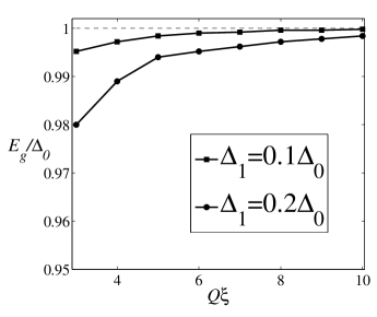
Figure 1: The energy gap, $E_{g}$, measured in units of $\Delta_{0}$, vs. $Q\xi$ for $Q\xi\gg 1$. The two curves are for $\Delta_{1}/\Delta_{0}=0.1$ and $0.2$, respectively. Here, $\Delta_{0}$ and $\Delta_{1}$ are the uniform and oscillating components of the order parameter, respectively. $Q$ is the modulating wavevector of the inhomogeneous coupling constant; $\xi$ is the superconducting coherence length. The estimated numerical error of $E_{g}/\Delta_{0}$ is about $0.01$. The deviation of $E_{g}$ from $\Delta_{0}$ is small, but it increases with larger $\Delta_{1}/\Delta_{0}$ or smaller $Q\xi$.

In real time, Eq. (3) becomes:

$$-\frac{D}{2}\partial_{x}^{2}\theta^{\prime} = \cos\theta^{\prime}(\Delta\cosh\theta^{\prime\prime}-E\sinh\theta^{\prime\prime}),$$

$$\frac{D}{2}\partial_{x}^{2}\theta^{\prime\prime} = \sin\theta^{\prime}(\Delta\sinh\theta^{\prime\prime}-E\cosh\theta^{\prime\prime}).$$ (18)

We numerically solved these coupled equations with periodic boundary condition on $[0,2\pi/Q]$, and computed the DOS $\nu(E)=\cos\theta_{1}\cosh\theta_{2}$, and thereby obtained the gap. We find that despite the fluctuating $\Delta(x)$, the energy gap, $E_{g}$, is spatially uniform. Fig. 1 shows a graph of $E_{g}$ vs. $Q\xi$ for $\Delta_{1}/\Delta_{0}=0.1$ and $0.2$. Again, in the plot we define the coherence length $\xi$ to be $\sqrt{\hbar D/\bar{\Delta}_{T=0}}=\sqrt{\hbar D/{\Delta_{0,T=0}}}$. One can see that in the limit $Q\xi\rightarrow\infty$ $E_{g}$ coincides with $\Delta_{0}$, and nonzero $1/(Q\xi)$ brings about only small corrections to make the gap slightly smaller than $\Delta_{0}$. These corrections increase with smaller $Q\xi$ or larger $U_{Q}/\bar{U}$ (i.e., $\Delta_{1}/\Delta_{0}$). Thus we find that for $Q\xi\gg 1$ case

$$\frac{2E_{g(T=0)}}{T_{c}}\lesssim\frac{2\Delta_{0(T=0)}}{T_{c}}=\frac{2\pi}{C}=3.52.$$ (19)

It is easy to understand the uniformity of $E_{g}$, since the wave function of a quasiparticle excitation should be extended on a length scale $1/Q\ll\xi$. Some intuition for the fact that $E_{g}\approx\Delta_{0}$ is provided in Sec. IV.

III.2 Slow pairing fluctuations: WKB-like local superconductivity

When the pairing strength fluctuates slowly, i.e., over a large distance, both the Green’s functions and the order parameter $\Delta(x)$ can vary on the length scale of $1/Q$, and we can approximate the zeroth order solution by a ’local solution’:

$$\theta_{0}(x)=\arctan\left(\frac{\Delta(x)}{\omega_{n}}\right),$$ (20)

where $\Delta(x)$ is to be solved from the self-consistency equation. This ’local’ property of the system implies a large spatial variation of both $\Delta(x)$ and $\theta(x)$, in contrast to the $Q\xi\gg 1$ case. To improve the zeroth order solution, we write $\theta(x)=\theta_{0}(x)+\theta_{1}(x)$. Neglecting the small gradient term of $\theta_{1}$, one can solve for $\theta_{1}$ from Usadel’s equation (3) :

$$\theta_{1}=\frac{D}{2}\left(\frac{\omega_{n}\partial_{x}^{2}\Delta}{(\Delta^{2}+\omega_{n}^{2})^{3/2}}-\frac{2\Delta\omega_{n}(\partial_{x}\Delta)^{2}}{(\Delta^{2}+\omega_{n}^{2})^{5/2}}\right),$$ (21)

thus the self-consistency equation (5) becomes

$$\Delta(x)=U(x)N_{F}2\pi T\sum_{n=0}^{\frac{\omega_{D}}{2\pi T}}\left(\frac{\Delta}{\sqrt{\Delta^{2}+\omega_{n}^{2}}}+\frac{\omega_{n}}{\sqrt{\Delta^{2}+\omega_{n}^{2}}}\theta_{1}\right).$$ (22)

In the Ginzburg-Landau regime, one is justified in keeping lowest order terms in (22):

$$\Delta(x)=U(x)N_{F}\left\{\Delta(x)\ln\left(\frac{2C\omega_{D}}{\pi T}\right)-\frac{7\zeta(3)}{8\pi^{2}T^{2}}\Delta^{3}(x)\right.$$

$$\left.+\frac{\pi\hbar D}{8T}\partial_{x}^{2}\Delta(x)\right\},$$ (23)

where $\zeta(n)$ is the Riemann $\zeta$ function. Remarkably, equation (III.2) is nothing but the Ginzburg-Landau equation for a modulating coupling constant $U(x)$ with $Q\xi\ll 1$, and is precisely the dirty case analogue of equation (9) in Ref. Martin et al., 2005, with $\xi$ replaced by the dirty limit expression ${\tilde{\xi}}^{2}=\hbar\pi D/8T$ ($\tilde{\xi}$ is slightly different from the coherence length defined in this work $\xi\equiv\sqrt{\hbar D/\bar{\Delta}_{T=0}}$, where $\bar{\Delta}$ is the spatially averaged $\Delta(x)$). In the limit $Q\xi\rightarrow 0$, $\Delta(x)$ would be determined only by the local value of $U(x)$, and the mean field transition temperature would be given by $T_{c,max}=2C\omega_{D}/\pi\exp(-1/(\bar{U}+U_{Q}))$. A small but nonzero $Q\xi$ leads to a weak coupling between spatial regions, hence slightly reducing the mean field $T_{c}$. Following the analysis of Ref. Martin et al., 2005, one obtains the mean field transition temperature:

$$T_{c}^{MF}\approx\frac{2C\omega_{D}}{\pi}e^{-{1}/{N_{F}(\bar{U}+U_{Q})}}e^{-\tilde{\xi}QA/\sqrt{2}},$$ (24)

where $A\equiv\sqrt{U_{Q}/(N_{F}\bar{U}^{2})}$.

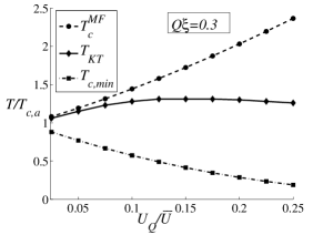
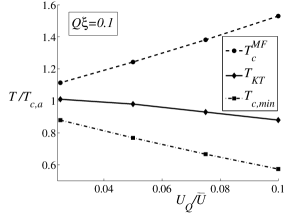
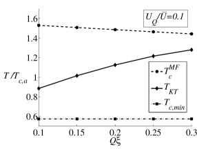
Figure 2: The mean field transition temperature $T_{c}^{MF}$, the Kosterlitz-Thouless temperature $T_{KT}$, and the minimum mean field transition temperature $T_{c,min}$ (see below) (a) vs. $U_{Q}/\bar{U}$ with $Q\xi=0.3$; (b) vs. $U_{Q}/\bar{U}$ with $Q\xi=0.1$; (c) vs. $Q\xi$ with $U_{Q}/\bar{U}=0.1$. In all cases $\bar{U}N_{F}=0.2$. $T$ is in units of $T_{c,a}\equiv\frac{2C}{\pi}\omega_{D}e^{-1/N_{F}\bar{U}}$. Dashed curve is $T_{c}^{MF}$ determined from equation (24); dash-dotted curve is the minimum mean field $T_{c}$ given by $T_{c,min}=\frac{2C}{\pi}\omega_{D}e^{-1/N_{F}(\bar{U}-|U_{Q}|)}$; solid curve is $T_{KT}$ obtained from numerically minimizing (25) and then solving (27). Here, $\bar{U}$ and $U_{Q}$ are the uniform and oscillating components of the coupling constant, respectively. $N_{F}$ is the density of states of the normal state; $Q$ is the modulating wavevector of the inhomogeneous coupling constant; $\xi$ is the superconducting coherence length. The estimated numerical error of $T_{KT}/T_{c,a}$ is about 0.01.

Although the inhomogeneous $U(x)$ largely increases the mean field $T_{c}$, it also makes the system more susceptible to phase fluctuations. This effect will be more pronounced in a two-dimensional superconductor, which we will focus on now. A film becomes superconducting through a Kosterlitz-Thouless transition. To determine the Kosterlitz-Thouless transition temperature, $T_{KT}$, we note that the Ginzburg-Landau free energy corresponding to (III.2) is

$$F(\Delta(x)) = N_{F}\int d^{3}x\{\alpha(x)\Delta^{2}(x)+\frac{\beta}{2}\Delta^{4}(x)$$ (25)

$$+ \gamma(\partial_{x}\Delta)^{2})\},$$

$$\alpha(x) = \frac{1}{N_{F}U(x)}-\ln\left(\frac{2\times 1.78\omega_{D}}{\pi T}\right),$$

$$\beta = \frac{7\zeta(3)}{8\pi^{2}T^{2}},\gamma=\frac{\pi\hbar D}{8T}.$$

As a functional of $\Delta(x)$, $F$ can be minimized numerically, thus giving a solution of $\Delta(x)$. The free energy cost for phase fluctuations is approximately $F=\frac{1}{2}\int d^{2}xJ(x)(\nabla\theta)^{2}$. For quasi-2d films,

$$J(x)=2N_{\bot}N_{F}^{2d}{\tilde{\xi}}^{2}|\Delta_{MF}(x)|^{2},$$ (26)

where $N_{F}^{2d}$ is the 2d electron DOS, $N_{\bot}$ is the number of channels, $\tilde{\xi}\equiv\sqrt{\frac{\pi\hbar D}{8T}}$, and $\Delta_{MF}$ is the mean field solution of (25). To explain the bilayer thin film experiments investigated by Long et al.Long et al. (2004, 2006), we use the measured value of the diffusion constant $D=5\times 10^{-3}m^{2}s^{-1}$ (see Ref. Long et al., 2004), and estimate $N_{\bot}=k_{F}d/\pi\approx 50$, where the film thickness $d\approx 10\sim 20$nmLong et al. (2004, 2006), and the Fermi wave vector $k_{F}\sim 1{\AA}^{-1}$. As in Ref. Martin et al., 2005, one can estimate $T_{KT}$ self-consistently from

$$T_{KT}=\frac{\pi}{2}\sqrt{\overline{J(x)}(\overline{1/J(x)})^{-1}},$$ (27)

since $\overline{J(x)}$ is the stiffness along the ”stripes”, while $(\overline{1/J(x)})^{-1}$ perpendicular to the ”stripes”. Although our estimation of $N_{\bot}$ is crude, the value of $T_{KT}$ is very insensitive to it. This is because $T_{KT}$ is solved self-consistently from (27). If one attempts to use a larger $N_{\bot}$ in (26), the enhancement of $T_{KT}$ is limited by $J(x)$ which itself is suppressed as temperature increases. Typical solutions of $T_{KT}$ are shown in FIG. 2. One can see that the phase fluctuation region, i.e. the difference between $T_{c}^{MF}$ and $T_{KT}$, increases with stronger inhomogeneity (FIG. 2(a) and (b)). Also for longer wave length modulation $T_{KT}$ is reduced more strongly (FIG. 2(c)). Heuristically, this is because for smaller $Q\xi$ the superconducting stripes become farther apart, and therefore it is more difficult for them to achieve phase coherence.

Moving our focus to the zero-temperature order parameter and gap, we note that at $T=0$ the integrals in equation (22) can be done:

$$\frac{\Delta(x)}{U(x)N_{F}}=\Delta(x)\ln\left(\frac{2\omega_{D}}{\Delta(x)}\right)+\frac{\pi D\partial_{x}^{2}\Delta}{8\Delta(x)}-\frac{\pi D(\partial_{x}\Delta)^{2}}{16\Delta^{2}(x)},$$

This can be approximately solved by:

$$\Delta(x) \approx \Delta_{0}(x)e^{-\eta(x)},$$ (28)

$$\Delta_{0}(x) = 2\omega_{D}e^{-\frac{1}{N_{F}U(x)}},$$

$$\eta(x) = \frac{\pi D}{8\Delta_{0}(x)}Q^{2}A^{2}\left(\cos(Qx)-\frac{1}{2}A^{2}\sin^{2}(Qx)\right).$$

Note that $\partial_{x}\Delta(x)\approx-A^{2}Q\sin(Qx)\Delta(x)$ [with $A$ defined under Eq. (24)], for our WKB analysis to be self-consistent, we need to require the that $A\lesssim\mathcal{O}(1)$, thus $U_{Q}/\bar{U}$ needs to be small. Also, when this is satisfied, $\eta(x)$ leads to a slight averaging between $\Delta(x)$, which is a manifestation of proximity effect.

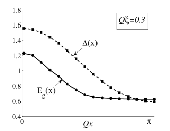
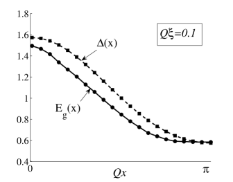
Figure 3: The local order parameter $\Delta(x)$ and the local gap $E_{g}(x)$ (in units of $\Delta(U_{Q}=0)=2\omega_{D}e^{-1/\bar{U}N_{F}}$) vs. spatial coordinate $x\in[0,\pi/Q]$. $Q\xi=0.3$ and $0.1$ in subfigure (a) and (b), respectively. $\bar{U}N_{F}=0.2$, $U_{Q}N_{F}=0.02$. Here, $\bar{U}$ and $U_{Q}$ are the uniform and oscillating components of the coupling constant, respectively. $N_{F}$ is the density of states of the normal state; $Q$ is the modulating wavevector of the inhomogeneous coupling constant; $\xi$ is the superconducting coherence length. The estimated numerical error of $E_{g}(x)$ is about $0.01$.

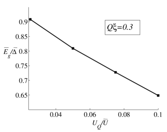
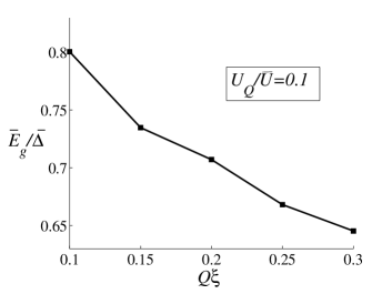
Figure 4: The ratios of the spatially averaged gap $\bar{E_{g}}$ to the spatially averaged $\bar{\Delta}$ (in units of $2\omega_{D}e^{-1/\bar{U}N_{F}}$) (a) vs. $U_{Q}/\bar{U}$ with $Q\xi=0.3$; (b) vs. $Q\xi$ with $U_{Q}/\bar{U}=0.1$. $\bar{U}N_{F}=0.2$ in all cases. Here, $\bar{U}$ and $U_{Q}$ are the uniform and oscillating components of the coupling constant, respectively. $N_{F}$ is the density of states of the normal state; $Q$ is the modulating wavevector of the inhomogeneous coupling constant; $\xi$ is the superconducting coherence length. The estimated numerical error is about 0.01.

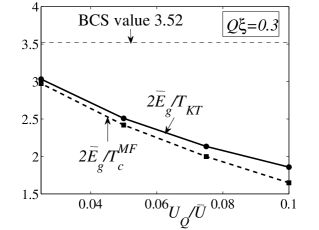
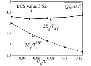
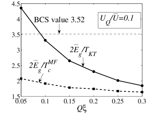
Figure 5: The ratios of the spatially averaged gap $\bar{E_{g}}$ to $T_{c}^{MF}$ or $T_{KT}$ (a)vs. $U_{Q}/\bar{U}$, $Q\xi=0.3$; (b) vs. $U_{Q}/\bar{U}$, $Q\xi=0.1$; (c) vs. $Q\xi$, $U_{Q}/\bar{U}=0.1$. In all cases $\bar{U}N_{F}=0.2$. Here, $\bar{U}$ and $U_{Q}$ are the uniform and oscillating components of the coupling constant, respectively. $N_{F}$ is the density of states of the normal state; $Q$ is the modulating wavevector of the inhomogeneous coupling constant; $\xi$ is the superconducting coherence length. The estimated numerical error is about 0.02.

To analyze the gap, we must switch to a real time formalism again, since our perturbative solution for the Green’s function becomes invalid as $E\rightarrow\Delta(x)$. Thus we have to solve the real time Usadel equation (III.1) with $\Delta(x)$ obtained above. Using the same numerical code as in Sec. III.1, we have obtained the local gap $E_{g}(x)$, which is plotted vs. $x$ in FIG. 3 for half a period of modulation. One can see that in general $E_{g}(x)$ is lower than $\Delta(x)$, and when $Q\xi=0.3$, $E_{g}(x)$ is largely set by the region with weakest coupling; but when $Q\xi\rightarrow 0$, $E_{g}(x)$ tends to follow much closer to $\Delta(x)$ as expected. In addition, the minimum of $E_{g}(x)$ is always slightly higher than the minimum of $\Delta(x)$ by an amount that also diminishes upon $Q\xi\rightarrow 0$. This behavior will be further clarified in the next section.

The ratio $\bar{E_{g}}/\bar{\Delta}$ vs. $U_{Q}/\bar{U}$ or $Q\xi$ is plotted in FIG. 4. The suppression of the gap strengthens when either the inhomogeneity becomes stronger ($U_{Q}/\bar{U}$ is large) or its length scale $L\sim 1/Q$ becomes smaller, consistent the results in FIG. 3. The $\bar{E_{g}}$ suppression relative to $\bar{\Delta}$, together with the fact the $T_{c}^{MF}$ is largely determined by strongest-coupling region, implies that the ratio $2\bar{E_{g}}/T_{c}^{MF}$ is generically reduced. The ratios $2\bar{E_{g}}/T_{c}^{MF}$ and $2\bar{E_{g}}/T_{KT}$ are plotted in FIG. 5 for several representative cases. As expected, there is always a strong suppression of the ratio $2\bar{E_{g}}/T_{c}^{MF}$ from $3.52$; for a two-dimensional system, however, the ratios with $T_{KT}$ are more subtle: for very small $Q\xi$ the ratio $2\bar{E_{g}}/T_{KT}$ might be enhanced due to the large deviation of $T_{KT}$ from $T_{c}^{MF}$ (see also FIG. 2(c)), while for larger value of $Q\xi$ the phase fluctuation region is narrow(see also FIG. 2(a)), and $2\bar{E_{g}}/T_{KT}$ is reduced from $3.52$.

For the purpose of comparison with the thin film experiments, a comment on the determination of $T_{c}^{MF}$ and $T_{KT}$ is in order. Due to disorder and phase fluctuations, the resistive transition curve can be significantly broadened. $T_{c}^{MF}$ can be estimated as the temperature at which the resistance drops to half of its normal state value, while $T_{KT}$ can be defined as the temperature at which the resistance drops below the measurement threshold (see, for example, Ref. Hsu et al., 1998). Alternatively, one can extract $T_{c}^{MF}$ from fitting the fluctuation resistance to Aslamazov-Larkin theoryAslamasov and Larkin (1968), and obtain $T_{KT}$ from nonlinear I-V characteristics or from fitting the resistance below $T_{c}^{MF}$ to Halperin-Nelson formHaperin and Nelson (1979) (see, e.g., Refs. Hebard and Paalanen, 1985; Mooij, 1984). Thus both $T_{c}^{MF}$ and $T_{KT}$ in principle can be measured from experiments, and can be used for comparison with our theoretical results here.

III.3 Additional inhomogeneities

Apart from modulation of the coupling $U$, one may also be interested in a simultaneous modulation of other properties. For example, in the small $Q\xi$ limit, one may expect the periodicity of $U$ to be accompanied by a periodicity of the local density of states at the fermi level, or the mean free path. Another possible modulation, that of a periodic potential, is suggested in Martin et al. (2005), and in practice is equivalent to local modulation of $U$. Indeed, one may use an effective description of the self consistency equation (5), taking $N_{F}\rightarrow N_{F}+N_{Q}\cos(Qx)$ to lowest order in the amplitude $N_{Q}$ of the local DOS in the form:

$$\Delta(\vec{r})={N_{F}}U_{mod}(\vec{r})\pi T\sum_{n}if_{\omega_{n}}(\vec{r}).$$ (29)

where $U_{mod}=\overline{U}+{N_{Q}\overline{U}+\overline{N_{F}}U_{Q}\over\overline{N_{F}}}\cos(Qx)$, and $N_{F}$ is the spatially averaged DOS. Formally this is exactly the same as Eq. (1), and can be treated similarly, taking

$$U_{Q}\rightarrow{N_{Q}\overline{U}+{N_{F}}U_{Q}\over{N_{F}}}$$ (30)

In practice, a local periodic potential may be imposed on the system externally by either acoustic means or an electromagnetic field. Thus it might be interesting to check the change in $T_{C}$ of a superconductor in the presence of an acoustic wave experimentally.

Another possibility of interest is that along with $U$ the electron mean-free path is modulated in the system. This can be naturally occurring if the periodicity in $U$ is a consequence of spatial variation in the properties of the material used. Alternatively, one may obtain this case by a periodic doping of the superconductor.

In this case we may describe the system effectively by modification of the Usadel equation (3) to:

$$-\frac{1}{2}\nabla\cdot(D\nabla\theta)=\Delta\cos\theta-\omega_{n}\sin\theta,$$ (31)

and taking the diffusion coefficient $D$ to be spatially dependent. Choosing $D=\overline{D}+D_{Q}\cos(Qx)$ and repeating the treatment above, we find that $D_{Q}$ does not change the values of the Green’s functions $\theta_{0},\theta_{1}$ above (It however appears at higher orders of the equation), and so doesn’t change the results of this paper within this order.

IV Superconductor-normal-metal (SN) superlattice analogy

Some insight into the nature of the lowest-lying excitations for both large and small $Q\xi$ cases can be gained by considering a simplified system: superconductor-normal-metal-superconductor (SNS) junctions. First, consider a single SNS junction with length $L=2\pi/Q$, and $\Delta(x)=\Delta$, $0$ in the S, N part respectively. Andreev bound states will form in the normal metal, and the energy of these states can be obtained by solving Bogoliubov-de Gennes (BdG) equations for the clean case, or Usadel equations for the dirty case. In the limit $L\rightarrow 0$, the energy of the lowest-lying state is $\Delta$, while in the opposite limit $L\gg\xi$, the (mini)gap is much smaller than $\Delta$: in the clean case $E_{g}\sim v_{F}/L\sim(Q\xi)\Delta$ and in the dirty case the gap equals the Thouless energy $D/L^{2}\sim(Q\xi)^{2}\Delta$ de Gennes (1964); Zagoskin (1998); Zhou et al. (1998). These states exponentially decay into the superconductors for a distance $\sim\xi$.

Based on a single SNS junction, one can build an SN superlattice with alternating superconductor and normal metal, each with length $L=2\pi/Q$, and $\Delta(x)=\Delta$, $0$ in the S, N part respectively. If $L\gg\xi$, Andreev bound states remain localized in the normal regions with the gap much smaller than $\Delta$. On the other hand if $L\ll\xi$, these states strongly mix with each other, and they form a tight-binding band. Therefore the gap, namely the lower band edge, is lower than $\Delta$, and in the limit $Q\xi\rightarrow\infty$ it is precisely at $\Delta/2$, the averaged $\Delta(x)$ (see the analytical calculation by Ref. van Gelder, 1969). The SN superlattice thus allows a qualitative understanding of the gap’s behavior in the problem we addressed above: if $Q\xi\gg 1$, all excitations are extended in space, with the uniform gap $E_{g}\approx\bar{\Delta}$; if $Q\xi\ll 1$, the lowest-lying excitations are localized in the weakest coupling regions whose gap is close to the minimum of $\Delta(x)$. This analogy also elucidates the features in FIG. 3: given a point in space $x_{0}$, $E_{g}(x_{0})$ is generally lower than $\Delta(x_{0})$, because the wave function of the low-lying excitations originating at a nearby region (within $\sim\xi$) with smaller $\Delta(x)$ are exponentially suppressed at $x_{0}$, and when $\xi$ is smaller this effect is reduced; thus $E_{g}(x)$ follows closer to $\Delta(x)$ in the limit $Q\xi\rightarrow 0$. Finally, the difference between the minimum of $E_{g}(x)$ and the minimum of $\Delta(x)$ resembles the minigap in SN superlattice $\sim v_{F}/L$ or $D/L^{2}$, which approaches zero as $Q\xi\rightarrow 0$.

V Summary and Discussion

In this paper we investigated the properties of dirty BCS superconductors with a fluctuating pairing coupling constant $U(x)=\bar{U}+U_{Q}\cos(Qx)$. Particularly, we analyzed the change in the mean field $T_{c}$, the zero-temperature order parameter $\Delta(x)$, and the energy gap in quasiparticle excitation $E_{g}(x)$ using the Usadel equation for quasiclassical Green’s functions. In addition, we estimated the Kosterlitz-Thouless transition temperature $T_{KT}$. Our analysis found four different regimes:
(1) $Q\xi\rightarrow\infty$. In this case the mean field $T_{c}$ and the spatially averaged order parameter $\bar{\Delta}$ are determined by the effective coupling constant $U_{eff}\gtrsim\bar{U}$ [see Eq. (15)]. Moreover, since in this regime any quasiparticle wavefunction is extended over the length scale $L=1/Q$, the local energy gap $E_{g}$ is uniform in space, and we found it to coincide with the spatially averaged $\bar{\Delta}$. The ratios $2\bar{\Delta}/T_{c}=2E_{g}/T_{c}=3.52$ maintain their universal BCS value.
(2) $Q\xi\gtrsim 1$. In this regime the physics is qualitatively the same as that of the previous case. The gap $E_{g}$, however, is smaller than $\bar{\Delta}$ by an amount that grows with decreasing $Q\xi$ or increasing $U_{Q}/\bar{U}$. Therefore $2\bar{E_{g}}/T_{c}\lesssim 3.52$ (see FIG. 1).
(3) $Q\xi\lesssim 1$. The system tends to divide into regions which behave according to the the local value of $U(x)$. Thus the mean field $T_{c}$ is determined by the first formation of local superconductivity upon lowering temperature, and therefore $T_{c}^{MF}$ is close to highest ’local $T_{c}$’. In contrast, the global energy gap or the spatially averaged local gap is largely determined by the region with smallest $U(x)$. Consequently, in this regime the ratio $2\bar{E_{g}}/T_{c}^{MF}$ is always suppressed from the universal BCS value, 3.52 (see FIG. 5a). Moreover, although the system is affected by phase fluctuations, in this regime $T_{KT}$ is close to $T_{c}^{MF}$ for small values of $U_{Q}$ (see FIG. 2a). Thus $2\bar{E_{g}}/T_{KT}$ is also smaller than 3.52 (see FIG. 5a).
(4) $Q\xi\rightarrow 0$. As opposed to the previous regime, here phase fluctuations lead to a large suppression of $T_{KT}$ relative to $T_{c}^{MF}$ (see FIG. 2b). Although $2\bar{E_{g}}/T_{c}^{MF}$ is still below 3.52, the ratios $2\bar{E_{g}}/T_{KT}$ is close to or larger than $3.52$ (see FIG. 5c).

The value of $2\bar{E_{g}}/T_{c}^{MF}$ and $2\bar{E_{g}}/T_{KT}$ vs. the entire range of $Q\xi$ is plotted schematically in FIG. 6, with regimes 1-4 explicitly labeled in the graph. Schematic results of $T_{c}^{MF}$ and $T_{KT}$ vs. $Q\xi$ are summarized in FIG. 7.

Figure 6: Schematic plot of the ratios $2\bar{E_{g}}/T_{c}^{MF}$ and $2\bar{E_{g}}/T_{KT}$ vs. $Q\xi$. Here $\bar{E_{g}}$ is the spatially averaged gap in local DOS; $T_{c}^{MF}$ is the mean field $T_{c}$; $T_{KT}$ is the Kosterlitz-Thouless transition temperature in 2d; $Q$ is the modulating wavevector of the inhomogeneous coupling constant; $\xi$ is the superconducting coherence length. 1,2,3, and 4 are labels of different regimes described in the text.

Figure 7: Schematic plot of the mean field transition temperature $T_{c}^{MF}$ and the Kosterlitz-Thouless temperature $T_{KT}$ vs. $Q\xi$, where $Q$ is the modulating wavevector of the inhomogeneous coupling constant; $\xi$ is the superconducting coherence length; $T_{c,max}=\frac{2C}{\pi}\omega_{D}e^{-1/N_{F}(\bar{U}+U_{Q})}$ is the maximum $T_{c}^{MF}$; $T_{c,a}\equiv\frac{2C}{\pi}\omega_{D}e^{-1/N_{F}\bar{U}}$ is the mean field $T_{c}$ for a uniform coupling $\bar{U}$. 1,2,3, and 4 are labels of different regimes described in the text. The qualitative feature of these results on $T_{c}$ are similar to those of Ref. Martin et al., 2005 on clean superconductors.

Finally, we discuss connections with thin film experiments Long et al. (2004, 2006). A straightforward realization of inhomogeneous coupling is in disordered superconductor-normal-metal (SN) bilayer thin films. In a homogeneous bilayer SN with thickness smaller than the coherence length $\xi$, mean field analysis yields that $T_{c}$ and the energy gap $E_{g}$ of the system are determined by the averaged coupling constant Cooper (1961); de Gennes (1964); Fominov and Feigel’man (2001)

$$U_{eff}=\frac{d_{S}N_{S}}{d_{S}N_{S}+d_{N}N_{N}}U,$$ (32)

where $U$ is the pairing coupling in the superconducting layer, $d$ is the thickness, $N$ is the DOS at the Fermi energy, and the subscripts $S$ and $N$ denote the superconductor and normal metal layers respectively. Thus the ratio $2E_{g(T=0)}/T_{c}$ is expected to remain at the BCS value $2\pi/C\approx 3.52$ in a homogeneous SN bilayers. Nevertheless, from (32) one observes that a spatially inhomogeneous thickness $d_{S,N}(x)$ (which is also consistent with the granular morphology of the sampleLong and J. M. Valles (2005)) leads to a nonuniform coupling $U(x)$ even if the original coupling $U$ is homogeneous. Therefore thickness variation generically leads to a superconductor with inhomogeneous pairing coupling. According to our results, a deviation of $2E_{g}/T_{c}$ from $3.52$ is expected in such a system.

Indeed our study was motivated by such observations. In Refs. Long et al., 2004, 2006 Long et al. report measurements of recently fabricated a series of Pb-Ag bilayer thin films, with thickness $d_{Pb}=4$nm and $d_{Ag}$ increases from $6.7$nm to $19.3$nm. They observed a significant reduction of $2\bar{E_{g}}/T_{c}^{MF}$ from the expected value $\sim 3.52$, where $\bar{E_{g}}$ is the spatially averaged gap extracted from tunneling measurement of the DOS, and $T_{c}^{MF}$ is measured as the temperature at which $R(T)$ drops to half of its normal state value, and the resistive transition is sharp and well-defined. This suppression of $2\bar{E_{g}}/T_{c}^{MF}$ is more pronounced in systems with thicker Ag thereby lower $T_{c}^{MF}$. In these samples with $T_{c}^{MF}$ decreasing from $2.55$K to $0.72$K with increasing $d_{Ag}$, the ratio $2\bar{E_{g}}/T_{c}^{MF}$ decreases from $\sim 3.6$ to $\sim 2.6$ (see FIG 3(b) of Ref. Long et al., 2006).

Figure 8: The ratios of the spatially averaged gap $\bar{E_{g}}$ to the mean field transition temperature $T_{c}^{MF}$ or the Kosterlitz-Thouless transition temperature $T_{KT}$ vs. $\bar{U}N_{F}$. $U_{Q}N_{F}=0.002$, $Q\xi=0.3$. Here, $\bar{U}$ and $U_{Q}$ are the uniform and oscillating components of the coupling constant, respectively. $N_{F}$ is the density of states of the normal state; $Q$ is the modulating wavevector of the inhomogeneous coupling constant; $\xi$ is the superconducting coherence length. Since $T_{c}^{MF}$ monotonically increases with $\bar{U}$, this result resembles the experimental data of Ref. Long et al., 2006 (see FIG. 3(b) ibid.), which shows that the lower the measured $T_{c}$ of a thin-film bilayer is, the smaller the ratio $2E_{g}/T_{c}$.The estimated numerical error is about 0.02.

These results can be qualitatively well understood by our study. The reduction of $2E_{g}/T_{c}^{MF}$ from $3.52$, together with the observed fact that the resistive transition is sharp and well-definedLong et al. (2004), implies that the experimental systems are in the regime (2) or (3) of our theoretical results summarized above (see FIG. 6). In these regimes both $2\bar{E_{g}}/T_{c}^{MF}$ and $2\bar{E_{g}}/T_{KT}$ are lower than $3.52$, and the phase fluctuation is either absent or small enough to keep $T_{KT}$ close to $T_{c}^{MF}$, explaining the sharp resistive transition. For samples with lower $T_{c}$, $\bar{U}$ is smaller. Therefore, if we assume roughly the same amount of $U_{Q}$ for all samples, the effect of inhomogeneity will be stronger for samples with lower $T_{c}$ samples, and, consequently, the gap-to-$T_{c}$ ratio is even smaller for them. To make a rough comparison, we have calculated the gap-$T_{c}$ ratio vs. $\bar{U}$ for fixed $U_{Q}$ and plotted the results in FIG. 8. Although not claiming more than a qualitative explanation of the bilayer measurements, we note that our FIG. 8 resembles FIG. 3(b) of Ref. Long et al., 2006.

An interesting venue for future research, which may extend to more 2d superconducting systems, is to consider a general fluctuation of the pairing interaction, not restricted to a particular wave number, but rather having a particular correlation length. In addition, aside from the low gap-$T_{c}$ ratio, Ref. Long et al., 2004 has also reported an unexpected subgap density of states of quasiparticles in the same bilayer materials. Although our current model does not produce this behavior, one expects that it could be explained by including large spatial fluctuations of the pairing interaction (e.g. $\frac{U_{Q}}{\bar{U}}\sim 1$), which strongly suppress the gap, and the effect of mesoscopic fluctuations which tend to produce subgap statesMeyer and Simons (2001).

Appendix A Calculation of $\Delta_{(T=0)}$ in the limit $Q\xi\gg 1$

Here we show some calculation details in deriving equation (III.1). At $T=0$ the self-consistency equations are

$$\Delta_{0}=N_{F}\bar{U}\left(\int_{0}^{\omega_{D}}d\omega\sin\theta_{0}\right)+\frac{N_{F}U_{Q}}{2}\left(\int_{0}^{\omega_{D}}d\omega\theta_{1}\cos\theta_{0}\right);$$

$$\frac{\Delta_{1}}{2}=\frac{N_{F}\bar{U}}{2}\left(\int_{0}^{\omega_{D}}d\omega\theta_{1}\cos\theta_{0}\right)+\frac{N_{F}U_{Q}}{2}\left(\int_{0}^{\omega_{D}}d\omega\sin\theta_{0}\right).$$

The evaluation of the integrals gives (define $a=\frac{DQ^{2}/2}{\Delta_{0}}$ and $x_{0}=\omega_{D}/\Delta_{0}$):

$$\int_{0}^{\omega_{D}}d\omega\sin\theta_{0}=\Delta_{0}\operatorname{arcsinh}\left(\frac{\omega_{D}}{\Delta_{0}}\right)\approx\Delta_{0}\ln\left(\frac{2\omega_{D}}{\Delta_{0}}\right);$$

$$\int_{0}^{\omega_{D}}d\omega\theta_{1}\cos\theta_{0} = \frac{\Delta_{1}}{2a}\left\{-2\arctan(x_{0})+2a\operatorname{arcsinh}(x_{0})\right.$$ (33)

$$- \sqrt{a^{2}-1}\left[\operatorname{arctanh}\left(\frac{x_{0}\sqrt{a^{2}-1}+1}{a\sqrt{x_{0}^{2}+1}}\right)\right.$$

$$+ \operatorname{arctanh}\left(\frac{x_{0}\sqrt{a^{2}-1}-1}{a\sqrt{x_{0}^{2}+1}}\right)$$

$$- \left.\left.2\operatorname{arctanh}\left(\frac{x_{0}}{\sqrt{a^{2}-1}}\right)\right]\right\}.$$

We take the limit $x_{0}=\frac{\omega_{D}}{\Delta_{0}}\gg 1$ and $a=(Q\xi)^{2}\gg 1$ simultaneously, but their relative ratio might be either large or small. Also using $\operatorname{arctanh}(z)=1/2\ln(|1+z|/|1-z|)$, one can show that in this limit the above integral equals

$$= \frac{\Delta_{1}}{2a}\left\{2a\ln(2x_{0})-a\left[\frac{1}{2}\ln\left(\frac{2x_{0}a}{\frac{a}{2x_{0}}+\frac{x_{0}}{2a}-1}\right)\right.\right.$$

$$+ \left.\left.\frac{1}{2}\ln\left(\frac{2x_{0}a}{\frac{a}{2x_{0}}+\frac{x_{0}}{2a}+1}\right)+\ln\left(\frac{|x_{0}-a|}{x_{0}+a}\right)\right]\right\}$$

$$= \frac{\Delta_{1}}{2}\left\{2\ln(2x_{0})-\left[\ln\left(\frac{2x_{0}a}{|\frac{x_{0}}{2a}-\frac{a}{2x_{0}}|}\right)+\ln\left(\frac{|x_{0}-a|}{x_{0}+a}\right)\right]\right\}$$

$$= \Delta_{1}\ln\left(1+\frac{x_{0}}{a}\right)=\Delta_{1}\ln\left(1+\frac{2\omega_{D}}{DQ^{2}}\right)=\frac{\Delta_{1}}{\bar{U}N_{F}}K_{1},$$

where $K_{1}$ has exactly the same form as defined in (13).

References

- Anderson (1959) P. W. Anderson, J. Phys. Chem. Solids 11, 26 (1959).
- Abrikosov and Gorkov (1959) A. A. Abrikosov and L. P. Gorkov, Sov. Phys. JETP 9, 220 (1959).
- Abrahams et al. (1979) E. Abrahams, P. W. Anderson, D. C. Licciardello, and T. V. Ramakrishnan, Phys. Rev. Lett 42, 673 (1979).
- Graybeal and Beasley (1984) J. M. Graybeal and M. R. Beasley, Phys. Rev. B 29, 4167 (1984).
- White et al. (1986) A. E. White, R. C. Dynes, and J. P. Garno, Phys. Rev. B 33, 3549 (1986).
- Dynes et al. (1986) R. C. Dynes, A. E. White, J. M. Graybeal, and J. P. Garno, Phys. Rev. Lett 57, 2195 (1986).
- Valles et al. (1989) J. M. Valles, R. C. Dynes, and J. P. Garno, Phys. Rev. B 40, 6680 (1989).
- Jaeger et al. (1989) H. M. Jaeger, D. B. Haviland, B. G. Orr, and A. M. Goldman, Phys. Rev. B 40, 182 (1989).
- Maekawa and Fukuyama (1981) S. Maekawa and H. Fukuyama, J. Phys. Soc. Jpn. 51, 1380 (1981).
- Anderson et al. (1983) P. W. Anderson, K. A. Muttalib, and T. V. Ramakrishnan, Phys. Rev. B 28, 117 (1983).
- Ma and Lee (1985) M. Ma and P. A. Lee, Phys. Rev. B 32, 5658 (1985).
- Kapitulnik and Kotliar (1985) A. Kapitulnik and G. Kotliar, Phys. Rev. Lett 54, 473 (1985).
- Ramakrishnan (1989) T. V. Ramakrishnan, Physica Scripta T27, 24 (1989).
- Finkel’stein (1987) A. M. Finkel’stein, JETP lett. 45, 46 (1987).
- Finkel’stein (1994) A. M. Finkel’stein, Physica B 197, 636 (1994).
- Larkin (1999) A. Larkin, Ann. Phys. (Leipzig) 8, 785 (1999).
- Ghosal et al. (2001) A. Ghosal, M. Randeria, and N. Trivedi, Phys. Rev. B 65, 014501 (2001).
- Dubi et al. (2007) Y. Dubi, Y. Meir, and Y. Avishai, Nature 449, 876 (2007).
- Fisher et al. (1990) M. P. A. Fisher, G. Grinstein, and S. M. Girvin, Phys. Rev. Lett. 64, 587 (1990).
- Haviland et al. (1989) D. B. Haviland, Y. Liu, and A. M. Goldman, Phys. Rev. Lett. 62, 2180 (1989).
- Hebard and Paalanen (1990) A. F. Hebard and M. A. Paalanen, Phys. Rev. Lett. 65, 927 (1990).
- Paalanen et al. (1992) M. A. Paalanen, A. F. Hebard, and R. R. Ruel, Phys. Rev. Lett. 69, 1604 (1992).
- Valles et al. (1992) J. M. Valles, R. C. Dynes, and J. P. Garno, Phys. Rev. Lett. 69, 3567 (1992).
- Liu et al. (1993) Y. Liu, D. B. Haviland, B. Nease, and A. M. Goldman, Phys. Rev. B 47, 5931 (1993).
- Hsu et al. (1995) S. Y. Hsu, J. A. Chervenak, and J. M. Valles, Phys. Rev. Lett. 75, 132 (1995).
- Valles et al. (1994) J. M. Valles, S. Y. Hsu, R. C. Dynes, and J. P. Garno, Physica B 197, 522 (1994).
- Yazdani and Kapitulnik (1995) A. Yazdani and A. Kapitulnik, Phys. Rev. Lett. 74, 3037 (1995).
- Hsu et al. (1998) S. Y. Hsu, J. A. Chervenak, and J. M. Valles, J. Phys. Chem. Solids 59, 2065 (1998).
- Goldman and Markovic (1998) A. M. Goldman and N. Markovic, Phys. Today 51, 39 (1998).
- Goldman (2003) A. M. Goldman, Physica E 18, 1 (2003).
- Sambandamurthy et al. (2004) G. Sambandamurthy, L. W. Engel, A. Johansson, and D. Shahar, Phys. Rev. Lett. 92, 107005 (2004).
- Fisher and Lee (1989) M. P. A. Fisher and D. H. Lee, Phys. Rev. B 39, 2756 (1989).
- Fisher (1990) M. P. A. Fisher, Phys. Rev. Lett. 65, 923 (1990).
- Wen and Zee (1990) X. G. Wen and A. Zee, Int. J. Mod. Phys. B 4, 437 (1990).
- Cha et al. (1991) M. C. Cha, M. P. A. Fisher, S. M. Girvin, M. Wallin, and A. P. Young, Phys. Rev. B 44, 6883 (1991).
- Wallin et al. (1994) M. Wallin, E. S. Sorensen, S. M. Girvin, and A. P. Young, Phys. Rev. B 49, 12115 (1994).
- Ephron et al. (1996) D. Ephron, A. Yazdani, A. Kapitulnik, and M. R. Beasley, Phys. Rev. Lett. 76, 1529 (1996).
- Mason and Kapitulnik (1999) N. Mason and A. Kapitulnik, Phys. Rev. Lett. 82, 5341 (1999).
- Mason and Kapitulnik (2001) N. Mason and A. Kapitulnik, Phys. Rev. B 64, 060504 (2001).
- Qin et al. (2006) Y. Qin, C. L. Vicente, and J. Yoon, Phys. Rev. B 73, 100505 (2006).
- Merchant et al. (2001) L. Merchant, J. Ostrick, R. P. Barber, and R. C. Dynes, Phys. Rev. B 63, 134508 (2001).
- Galitski et al. (2005) V. M. Galitski, G. Refael, M. P. A. Fisher, and T. Senthil, Phys. Rev. Lett. 95, 077002 (2005).
- Dalidovich and Phillips (2001) D. Dalidovich and P. Phillips, Phys. Rev. B 64, 052507 (2001).
- Spivak et al. (2001) B. Spivak, A. Zyuzin, and M. Hruska, Phys. Rev. B 64, 132502 (2001).
- Kapitulnik et al. (2001) A. Kapitulnik, N. Mason, S. A. Kivelson, and S. Chakravarty, Phys. Rev. B 63, 125322 (2001).
- Shimshoni et al. (1998) E. Shimshoni, A. Auerbach, and A. Kapitulnik, Phys. Rev. Lett. 80, 3352 (1998).
- Dubi et al. (2006) Y. Dubi, Y. Meir, and Y. Avishai, Phys. Rev. B 73, 054509 (2006).
- Long et al. (2004) Z. Long, J. M. D. Stewart, T. Kouh, and J. J. M. Valles, Phys. Rev. Lett 93, 257001 (2004).
- Long et al. (2006) Z. Long, J. M. D. Stewart, and J. J. M. Valles, Phys. Rev. B 73, 140507 (2006).
- Cooper (1961) L. N. Cooper, Phys. Rev. Lett 6, 689 (1961).
- de Gennes (1964) P. G. de Gennes, Rev. Mod. Phys. 36, 225 (1964).
- Fominov and Feigel’man (2001) Y. V. Fominov and M. V. Feigel’man, Phys. Rev. B 63, 094518 (2001).
- Abrikosov (1988) A. A. Abrikosov, Fundamental Theory of Metals (North-Holland, 1988).
- Martin et al. (2005) I. Martin, D. Podolsky, and S. A. Kivelson, Phys. Rev. B 72, 060502 (2005).
- Larkin and Ovchinnikov (1972) A. I. Larkin and Y. N. Ovchinnikov, Sov. Phys. JETP 34, 1144 (1972).
- Meyer and Simons (2001) J. S. Meyer and B. D. Simons, Phys. Rev. B 64, 134516 (2001).
- Aryanpour et al. (2006) K. Aryanpour, E. R. Dagotto, M. Mayr, T. Paiva, W. E. Pickett, and R. T. Scalettar, Phys. Rev. B 73, 104518 (2006).
- Loh and Carlson (2007) Y. L. Loh and E. W. Carlson, Phys. Rev. B 75, 132506 (2007).
- Usadel (1970) K. D. Usadel, Phys. Rev. Lett 25, 507 (1970).
- Kopnin (2001) N. B. Kopnin, Theory of Nonequilibrium Superconductivity (Oxford University Press, 2001).
- Belzig et al. (1999) W. Belzig, F. Wilhelm, G. Schon, C. Bruder, and A. Zaikin, Superlattices and Microstructures 25, 1251 (1999).
- Aslamasov and Larkin (1968) L. G. Aslamasov and A. I. Larkin, Phys. Lett. 26A, 238 (1968).
- Haperin and Nelson (1979) B. I. Haperin and D. R. Nelson, J. Low. Temp. Phys. 36, 599 (1979).
- Hebard and Paalanen (1985) A. F. Hebard and M. A. Paalanen, Phys. Rev. Lett. 54, 2155 (1985).
- Mooij (1984) J. E. Mooij, in Percolation, Localization, and Superconductivity, edited by A. M. Goldman and S. A. Wolf (Plenum Press, 1984).
- Zagoskin (1998) A. M. Zagoskin, Quantum Theory of Many-Body Systems (Springer, 1998).
- Zhou et al. (1998) F. Zhou, P. Charlat, B. Spivak, and B. Pannetier, Journal of Low Temperature Physics 110, 841 (1998).
- van Gelder (1969) A. P. van Gelder, Phys. Rev. 181, 787 (1969).
- Long and J. M. Valles (2005) Z. Long and J. J. M. Valles, J. Low. Temp. Phys. 139, 429 (2005).