Features of Traffic Congestion caused by bad Weather Conditions or Accidents

Abstract

Spatiotemporal features and physics of vehicular traffic congestion occurring due to heavy freeway bottlenecks caused by bad weather conditions or accidents are found based on simulations in the framework of three-phase traffic theory. A model of a heavy bottleneck is presented. Under a continuous non-limited increase in bottleneck strength, i.e., when the average flow rate within a congested pattern allowed by the heavy bottleneck decreases continuously up to zero, the evolution of the traffic phases in congested traffic, synchronized flow and wide moving jams, is studied. It is found that at small enough flow rate within the congested pattern, the pattern exhibits a non-regular structure: a pinch region of synchronized flow within the pattern disappears and appears randomly over time; some of the wide moving jams merge randomly into a mega-wide moving jam (mega-jam). We show that the smaller the average flow rate allowed by the heavy bottleneck within the congestion, the less the mean pinch region width and the greater the mean mega-jam width; when the bottlenecks strength increases further, only the mega-jam survives and synchronized flow remains only within its downstream front separating free flow and congested traffic. Theoretical results presented explain empirical complexity of traffic congestion caused by bad weather conditions or accidents.

1 Introduction

The physics of freeway traffic congestion is one of the most quickly developed fields of complex spatiotemporal systems. In empirical observations, traffic breakdown (onset of congestion) in free flow occurs mostly at bottlenecks associated with, e.g., on- and off-ramps. In congested traffic, moving jams are observed [1, 2, 3, 4, 5, 6, 7, 8, 9, 10, 11, 12]. A moving jam is a localized structure of great vehicle density, spatially limited by two jam fronts; the jam propagates upstream; within the jam vehicle speed is very low.

Moving jams, which exhibit a characteristic jam feature [J] to propagate through bottlenecks while maintaining the mean velocity of the downstream jam front, are called wide moving jams [12]. A wide moving jam consists of alternations of regions in which traffic flow is interrupted and moving blanks [13, 14]; a moving blank is a blank between vehicles, which moves upstream due to vehicle motion within the jam. The flow interruption can be used as a microscopic criterion for a wide moving jam associated with the jam definition [J] [13, 14].

In observations [12], traffic breakdown is associated with a local first-order phase transition from free flow to synchronized flow (F$\rightarrow$S transition) at the bottleneck; synchronized flow [S] is defined as congested traffic that does not exhibit the feature [J]; in particular, the downstream front of synchronized flow is often fixed at the bottleneck. Wide moving jams can emerge spontaneously in synchronized flow (S$\rightarrow$J transition) only, i.e., due to a sequence of F$\rightarrow$S$\rightarrow$J transitions.

Moving jam emergence in synchronized flow leading to S$\rightarrow$J transitions is called the pinch effect occurring within an associated pinch region of synchronized flow (see Sect. 12.2 of [12]): (i) The density increases and average speed decreases; narrow moving jams, which do not exhibit the feature [J], appear in the pinch region. (ii) These jams propagate upstream growing in their amplitude; as a result, S$\rightarrow$J transitions occur, i.e., wide moving jam emerge. The upstream boundary of the pinch region is a road location at which a narrow moving jam has just transformed into a wide moving one. (iii) These locations can vary for different wide moving jams, i.e., the pinch region width depends on time. A congested traffic pattern that exhibits this regular structure is called a general pattern (GP).

Earlier traffic flow theories and models reviewed in [1, 2, 3, 4, 5, 6, 7, 8, 9, 10] cannot explain F$\rightarrow$S$\rightarrow$J transitions and the pinch effect (see a criticism of the theories in Ref. [12, 15]). For this reason, the author introduced a three-phase traffic theory (references in [12]) in which there are (i) the free flow, (ii) synchronized flow, and (iii) wide moving jam phases. The synchronized flow and wide moving jam phases associated with congested traffic are defined via the empirical definitions [S] and [J], respectively. The first three-phase traffic flow models showing the pinch effect are stochastic microscopic models [16, 17]. Later, other three-phase traffic flow models were developed [18, 19, 20, 15, 21, 22].

In general, the average flow rate $q^{\rm(cong)}$  within a congested traffic pattern upstream of a bottleneck is the smaller, the greater the bottleneck influence of traffic (called the bottleneck strength). Empirical data show that the flow rate $q^{\rm(cong)}$ within GPs occurring at usual bottlenecks like on- and off-ramp bottlenecks, which is equal to the average flow rate in the pinch region $q^{\rm(pinch)}$, is approximately within a range

$$q^{\rm(cong)}=q^{\rm(pinch)}=1100-1700\ {\rm vehicles/h/lane}.$$ (1)

Features of GPs and other congested patterns occurring at usual bottlenecks determined by road infrastructure (on- and off-ramps, road gradients, etc.), for which condition (1) is valid, have already been studied in detail [12]. In contrast with the usual bottlenecks, due to bad weather conditions or accidents heavy bottlenecks can occur, which exhibit a much greater influence on traffic (greater bottleneck strength) that limits $q^{\rm(cong)}$ to very small values, sometimes as low as zero. Features of traffic congestion at the heavy bottlenecks are unknown.

As follows from recent empirical studies of sequences of wide moving jams [13, 14], the flow rate $q^{\rm(blanks)}$ of low speed states associated with moving blanks within the jams is approximately within a range

$$q^{\rm(blanks)}=300-600\ {\rm vehicles/h/lane}.$$ (2)

The flow rate between the jams associated with non-interrupted flows in the jams’ outflows $q^{\rm(J)}_{\rm out}$ is greater than $q^{\rm(pinch)}$ (1), i.e., $q^{\rm(J)}_{\rm out}$ is considerably greater than $q^{\rm(blanks)}$ (2). Now we assume that due to bad weather conditions or an accident a heavy bottleneck occurs with a great strength for which

$$q^{\rm(cong)}\rightarrow q^{\rm(blanks)}.$$ (3)

In this case, $q^{\rm(J)}_{\rm out}$ must reduce to $q^{\rm(blanks)}$ (2), i.e., the difference between flows within and outside wide moving jams disappears. As a result, all wide moving jams should merge into one mega-wide moving jam (mega jam for short). Thus already from this qualitative consideration, we can expect interesting physical phenomena associated with complexity of traffic congestion at heavy bottlenecks.

In this letter, we reveal these features and compare them with measured congested patterns at heavy bottlenecks caused by bad weather conditions or accidents.

2 A Theory of Traffic Congestion at Heavy Bottlenecks

For a theoretical analysis of traffic congestion at heavy bottlenecks, we use a stochastic three-phase traffic flow model of a two-lane road [16, 23] (see Appendix) with the following heavy bottleneck model.

We suggest that there is a section of the road within which due to an accident or bad weather conditions drivers should increase a safety time gap $\tau^{\rm(safe)}$ to the preceding vehicle. We simulate this effect by an increase in $\tau^{\rm(safe)}$ to some $\tau^{\rm(safe)}=T_{\rm B}>$ 1 sec in comparison with $\tau^{\rm(safe)}=$ 1 sec used in the model for vehicles moving outside this section. In according with Eq. (18) of the model (Appendix), $\tau^{\rm(safe)}$ determines a safe speed, which should not be exceeded by a driver; otherwise, the driver decelerates. As a result, within this section drivers move with time headways that are approximately equal to $\tau^{\rm(safe)}=T_{\rm B}$. Therefore the section with longer $\tau^{\rm(safe)}=T_{\rm B}$ acts as a bottleneck on the road. In the bottleneck model suggested here, each chosen value $T_{\rm B}$ defines a specific bottleneck: the strength of this bottleneck is the greater, the longer $T_{\rm B}$; in turn, the longer $T_{\rm B}$, the smaller $q^{\rm(cong)}$, i.e., the greater the flow rate limitation within congestion caused by the bottleneck. This model feature allows us to simulate a heavy bottleneck caused by bad weather conditions or accidents leading to a long enough $T_{\rm B}$ within the bottleneck .

When $T_{\rm B}$ is chosen to be not very long, then at a great enough flow rate $q_{\rm in}$ in free flow upstream of the bottleneck, firstly an F$\rightarrow$S transition occurs spontaneously at the bottleneck. Then the pinch region with a relatively great flow rate $q^{\rm(cong)}=q^{\rm(pinch)}$ is formed. At the pinch region upstream boundary wide moving jams emerge. Thus we found known phenomena of regular GP formation (Figs. 1 (a), 2 and 3 (a, b)) [12]. The pinch region width $L^{\rm(pinch)}(t)$ changes over time between about 1 and 2 km (Fig. 4 (a)). $L^{\rm(pinch)}$ is defined as the distance between the upstream boundary of the bottleneck ($x=$ 16 km) and the road location upstream at which a wide moving jam has just been identified through the use of the jam microscopic criterion. There is also a nearly constant frequency of $L^{\rm(pinch)}(t)$ oscillations associated with the maximum in the Fourier spectrum (Fig. 4 (b)). Speed autocorrelation functions and associated Fourier spectra of speed time-dependencies at shorter $T_{\rm B}$ show regular character of wide moving jam propagation (Fig. 3 (c, d)).

When $T_{\rm B}$ increases and therefore $q^{\rm(cong)}=q^{\rm(pinch)}$ decreases (Fig. 2), and $T_{\rm B}$ remains a relatively small value ($1.8<T_{\rm B}<3$ sec), then as for other bottleneck types, we found the following known GP features [12]: the smaller the flow rate $q^{\rm(pinch)}$, the greater the frequency of narrow moving jam emergence within the pinch region, the lower the maximum speed between wide moving jams upstream of the pinch region, the smaller the mean pinch region width $L^{\rm(pinch)}_{\rm mean}$ (Figs. 1 (b) and 4 (c, d, i)). This can also be seen from a comparison of time-dependences of average speed within the region of wide moving jams for different $T_{\rm B}$ (Fig. 3 (a, e)).

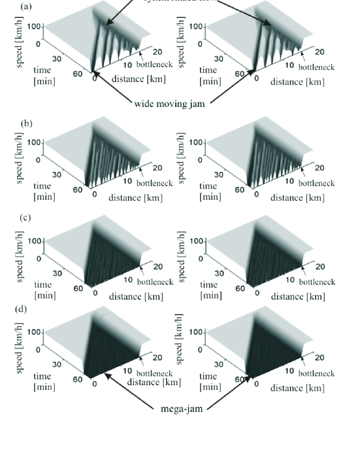
Figure 1: Simulated speed in space and time in the left (left) and right (right) road lanes at different $T_{\rm B}$: $T_{\rm B}=$ 1.8 (a), 2.4 (b), 12 (c), 30 sec (d). $q_{\rm in}=$ 1946 vehicles/h/lane. The upstream boundary of bottleneck region of the length 300 m is at $x=$ 16 km; the maximum speed w thin this region is 60 km/h. Resulting values of $q^{\rm(cong)}=$ 1546 (a), 1114 (b), 440 (c), 217 vehicles/h/lane (d).

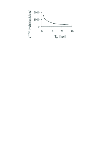
Figure 2: Simulated average flow rate $q^{\rm(cong)}$ within congested patterns shown in Fig. 1 as a function of $T_{\rm B}$ . The averaging time interval for $q^{\rm(cong)}$ is 60 min.

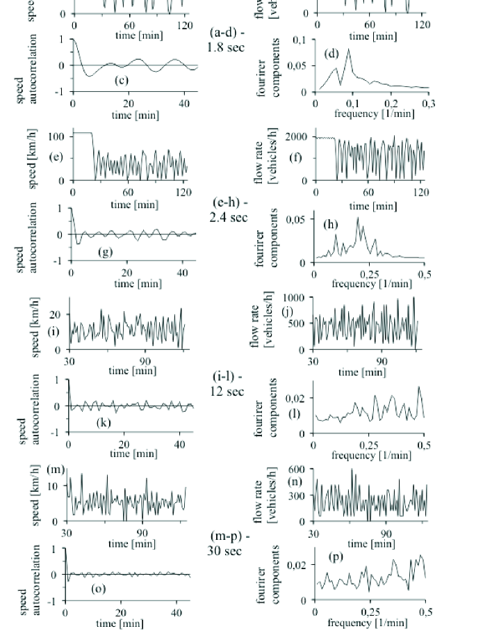
Figure 3: Characteristics of congested patterns shown in Fig. 1 related to location 10 km. Time-functions of speed (a, e, i, m), speed correlations (c, g, k, o), associated Fourier spectra (d, h, l, p), and flow rate (b, f, j, n) for different $T_{\rm B}=$ 1.8 (a-d), 2.4 (e-h), 12 (i-l), 30 sec (m-p). 1-min average data.

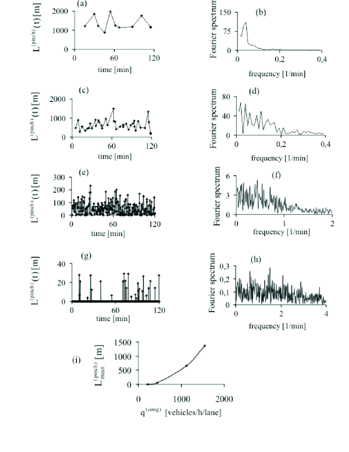
Figure 4: Simulations of pinch effect: $L^{\rm(pinch)}(t)$ (a, c, e, g), associated Fourier spectra (b, d, f, h) for congested patterns shown in Fig. 1, $L^{\rm(pinch)}_{\rm mean}(q^{\rm(cong)})$ (i). In (a–h) $T_{\rm B}=$ 1.8 (a, b), 2.4 (c, d), 12 (e, f), 30 sec (g, h).

Qualitatively other phenomena are found when $T_{\rm B}$ further increases ($T_{\rm B}>3$ sec) and the average flow rate $q^{\rm(cong)}$ decreases considerably (Figs. 1 (c, d) and 2). Firstly, $L^{\rm(pinch)}(t)$ becomes a non-regular time-function (Fig. 4 (e, g)) whose Fourier spectrum is broader, the longer $T_{\rm B}$ (Fig. 4 (f, h)); there are random time intervals when the pinch region disappears, i.e., $L^{\rm(pinch)}=0$ (Fig. 4 (e)). This means that there are time instants at which there is no pinch region and wide moving jams emerge directly at the upstream boundary of the bottleneck, whereas for other time intervals the pinch region appears again (Fig. 4 (e)). Consequently, $L^{\rm(pinch)}_{\rm mean}$ decreases continuously, when $T_{\rm B}$ increases (Fig. 4 (i)). $L^{\rm(pinch)}_{\rm mean}$ reaches almost zero for $T_{\rm B}=$ 30 sec: for such a heavy bottleneck, the pinch region does not exist.

When $T_{\rm B}$ increases and the pinch region disappears during some random time intervals, the GP behaviour qualitatively changes: the time-functions of average speed become non-regular ones (Fig. 3 (i, m)). We found that under condition (3), the pinch region disappears and wide moving jams merge into a mega-jam. In particular, for $T_{\rm B}=$ 30 sec no separated wide moving jams can be distinguished: instead of the sequence of wide moving jams, a mega-jam occurs only. These effects can also be seen from speed autocorrelation functions and associated Fourier spectra of the average speed time-dependences (Fig. 3 (k, l, o, p)). The mega-jam is found at those long values of $T_{\rm B}$ at which the pinch region disappears. Simulations show that the mega-jam consists of alternations of flow interruption and low speed states associated with moving blanks. Thus there are no continuous flows within the congested pattern any more with the one exception of the downstream front of synchronized flow that separates free flow downstream and the mega-jam upstream of the front. Synchronized flow remains only within this front. Thus in accordance with all known empirical data and theoretical results presented, the condition

$$q^{\rm(cong)}>q^{\rm(blanks)}$$ (4)

is a necessary condition for GP existence at a bottleneck.

For explanations of these results, we recall that an S$\rightarrow$J transition is a first-order phase transition [12], i.e., it is characterized by a random time delay $T_{\rm SJ}$. $T_{\rm SJ}$ includes a random time delay of spontaneous nucleation of a narrow moving jam (nucleus for the S$\rightarrow$J transition) and its random growth within the pinch region until the jam transforms into a wide moving jam at the upstream boundary of the pinch region. Thus the smaller $T_{\rm SJ}$, the shorter $L^{\rm(pinch)}$. The random character of $T_{\rm SJ}$ explains a time-dependence of $L^{\rm(pinch)}(t)$ (Fig. 4 (c, e)). We found that the greater $T_{\rm B}$, the greater the density within the pinch region and the smaller the mean random time delay $T^{\rm(mean)}_{\rm SJ}$. Thus the greater $T_{\rm B}$, the greater the probability for the occurrence of a negligibly small $T_{\rm SJ}$ and wide moving jam emergence directly upstream of the synchronized flow front; in the latter case $L^{\rm(pinch)}=$ 0. This explains also why $L^{\rm(pinch)}_{\rm mean}$ decreases up to zero, when an increase in $T_{\rm B}$ causes a decrease in $T^{\rm(mean)}_{\rm SJ}$ up to zero, i.e., when all wide moving jams emerge almost directly upstream of the bottleneck and the pinch region disappears.

When $q^{\rm(cong)}$ becomes zero, because behind a road location the road is closed, the mega-jam transforms into a queue of motionless vehicles, which therefore is not associated with vehicular traffic. Nevertheless, there is a link between the queue and the mega-jam. If at a time instant we allow several vehicles to escape from this queue, then simulations show that motion of these vehicles results in wide moving jam occurrence: the downstream front of the jam separates moving vehicles escaping from the queue and vehicles standing within the queue upstream of the front. When the number of vehicles escaping from the initial queue decreases, the downstream jam front transforms into a moving blank(s) subsequently covered by vehicles standing in the queue. When a vehicle per a long enough time interval is allowed to escape from the mega-jam, as simulations show, a sequence of such moving blanks within this jam occur; these moving blanks exhibit, however, dynamics specifically associated with the mega-jam.

Thus based on a study of three-phase traffic flow model we found that the complexity of traffic congestion caused by bad weather conditions or accidents, when a very heavy bottleneck appears on a road, is associated with the phenomenon of random disappearance and appearance of the pinch region over time that is accompanied by the random merger of some wide moving jams into a mega-jam. When the bottleneck strength increases further strongly, the pinch region disappears and only the mega-jam survives and synchronized flow remains only within its downstream front separating free flow and congested traffic. These phenomena explained by random nucleation of moving jams in congested traffic reveal the evolution of the traffic phases when heavy bottlenecks occur in highway traffic.

3 Discussion. Comparison with Empirical Results

To compare the above theory of traffic congestion with empirical congested patterns, one should have measured data for traffic congestion at a bottleneck, whose strength should be manually continuously changeable from the one associated with usual bottlenecks like on- and off-ramps to great bottleneck strengths associated with heavy bottlenecks caused by bad weather conditions or accidents. Unfortunately, such measured data is not available. However, we can compare the theory with measured data related to two limiting cases: (i) Traffic congestion at an usual on-ramp bottleneck (Fig. 5). (ii) Traffic congestion at a heavy bottleneck caused by bad weather conditions – snow and ice on a road (Fig. 6).

The speed distributions with congested patterns found in simulations (Fig. 1 (a, b)) for the range of $T_{\rm B}=1.6-2.4$ sec associated with the flow rate range

$$q^{\rm(cong)}=q^{\rm(pinch)}=1120-1800\ {\rm vehicles/h/lane}$$ (5)

are qualitatively the same as those in an empirical GP shown in Fig. 5 and in all other known empirical GPs [12]. Moreover, quantitative values of empirical flow rates $q^{\rm(pinch)}$ (1) are approximately associated with the theoretical result (5). In particular, within the pinch region of the GP shown in Fig. 5 (a), the flow rate averaged between 7:00 and 8:00 and across the road is $q^{\rm(pinch)}=1200$ vehicles/h/lane.

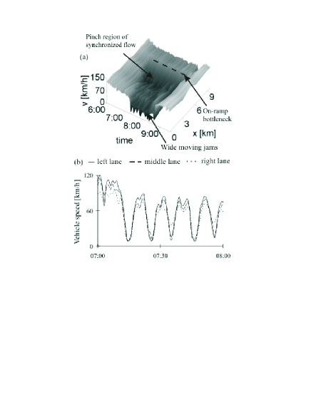
Figure 5: Usual empirical traffic congestion – a general pattern (GP) at on-ramp bottleneck: (a) Speed in space and time for the GP. (b) Speed in different lanes within a sequence of wide moving jams associated with (a) at location 1.5 km. 1-min average data measured on the freeway A5-South in Germany dated April 15, 1996. Arangement of detectors is shown in Fig. 2.1 of the book [12].

In contrast, for $T_{\rm B}\geq$ 6 sec associated with the average flow rate

$$q^{\rm(cong)}\leq 625\ {\rm vehicles/h/lane}$$ (6)

the theoretical speed patterns (Fig. 1 (c, d)) are qualitatively the same as those we found in empirical data measured on many various days (and years) on different freeways, when very heavy bottlenecks caused by bad weather conditions or accidents occur for which empirical flow rates $q^{\rm(cong)}<700$ vehicles/h/lane. In this case, rather than regular structure of traffic congestion of GPs (Figs. 1 (a, b) and 5), both empirical and theoretical traffic congested patterns (Figs. 1 (c, d) and 6) exhibit non-regular spatiotemporal structure of congestion in which no sequences of wide moving jams can be distinguished. In addition, the mentioned empirical flow rates $q^{\rm(cong)}<700$ vehicles/h/lane found within the empirical non-regular congested patterns are associated with the theoretical result (6). In turn, these theoretical and empirical results for $q^{\rm(cong)}$ correspond to empirical flow rates found within wide moving jams associated with moving blanks (2).

An example of such an empirical congested traffic pattern is shown in Fig. 6. Indeed, rather than the regular structure of congestion within the GP (Fig. 5), in measured data associated with bad weather conditions a non-regular spatiotemporal structure of congestion is observed (Fig. 6). A heavy bottleneck appears on February 02, 2006 between locations 4.07 and 3.02 km due to snow and ice. Upstream of the bottleneck, very low speed and flow rate patterns ($x\leq$ 3.02 km in Fig. 6 (b)) are observed. Downstream of the bottleneck ($x=$ 4.07 km) vehicles have escaped from the congestion (speed is high), however, the flow rate is very small because the bottleneck reduced the average flow rate within the congestion strongly. For example, at $x=$ 3.02 km, the flow rate $q^{\rm(cong)}$ averaged between 7:00 and 7:40 and across the road is only 513 vehicles/h/lane that corresponds to the theoretical result (6). In contrast with the GP in Fig. 5 (b) (as with other empirical GPs [12]), within traffic congestion shown in Fig. 6 (b) non-regular low speed patterns are observed in which a sequence of wide moving jams cannot be distinguished ($x\leq$ 3.02 km). This conclusion is regardless of the flow rates to on- and off-ramps, which in the data set lead to a greater average flow rate downstream of the freeway intersection (Fig. 6 (a, b)).

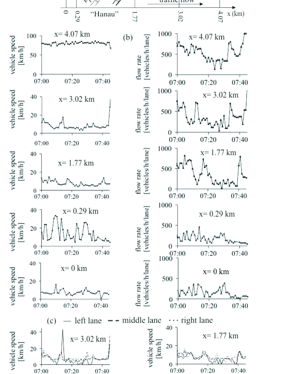
Figure 6: Empirical structure of congestion caused by snow and ice: (a) Schema of road detector arrangement on a section of the freeway A3-North in Germany near the intersection $``$Hanau”. (b) Average speed and flow rate across the freeway at different locations. (c) Speed in different lanes at two locations. 1-min average data.

If speeds in different lanes are compared (Fig. 6 (c)), we find even more non-regular speed time-dependencies: whereas no vehicles pass a detector in one of the lanes, i.e., the speed is zero, during the same time interval the average speed in other lanes can be higher than zero. This explains why in time-dependences of speeds averaged across the road (Fig. 6 (b)), this very low speed is seldom equal to exactly zero.

I thank Sergey Klenov for help in simulations, Ines Maiwald-Hiller for help in data analysis, Andreas Hiller, Gerhard Nöcker, Hubert Rehborn and Olivia Brickley for suggestions.

Appendix A Stochastic Microscopic Three-Phase Traffic Flow Model

The stochastic microscopic three-phase traffic flow model for two-lane road used in all simulations presented above reads as follows [16, 23]:

$$v_{n+1}=\max(0,\min({v_{\rm free},\tilde{v}_{n+1}+\xi_{n},v_{n}+a\tau,v_{{\rm s},n}})),$$ (7)

$$x_{n+1}=x_{n}+v_{n+1}\tau,$$ (8)

$$\tilde{v}_{n+1}=\max(0,\min({v_{\rm free},v_{{\rm c},n},v_{{\rm s},n}})),$$ (9)

(10)

$$v_{c,n}=\left\{\begin{array}[]{ll}v_{n}+\Delta_{n}&\textrm{at $g_{n}\leq G_{n}$}\\ v_{n}+a_{n}\tau&\textrm{at $g_{n}>G_{n}$},\end{array}\right.$$ (13)

where

$$\Delta_{n}=\max(-b_{n}\tau,\min(a_{n}\tau,\ v_{\ell,n}-v_{n})),$$ (14)

where index $n$ corresponds to the discrete time $t=n\tau$, $n=0,1,2,...;$ $\tau$ is time step; $v_{\rm n}$ is the vehicle speed at time step $n$; $x_{n}$ is the vehicle co-ordinate; $\tilde{v}_{\rm n}$ is the speed calculated without a noise component $\xi_{n}$; $v_{\rm free}$ is the maximum speed in free flow that is constant; $a$ is the maximum acceleration; $g_{n}=x_{\ell,n}-x_{n}-d$ is the space gap; the lower index $\ell$ marks functions and values related to the preceding vehicle; $v_{\rm s,n}$ is a safe speed; all vehicles have the same length $d$; $a_{n}\geq 0$, $b_{n}\geq 0$ (see below); $G_{n}$ is a synchronization gap:

$$G_{n}=G(v_{n},v_{\ell,n}),$$ (15)

where the function $G(u,w)$ is chosen as

$$G(u,w)=\max(0,k\tau u+\phi_{0}a^{-1}u(u-w)),$$ (16)

$k>1$ and $\phi_{0}$ are constants.

The safe speed $v_{{\rm s},n}$ in (7) is chosen in the form

$$v_{{\rm s},n}=\min{(v^{\rm(safe)}_{n},g_{n}/\tau+v^{\rm(a)}_{\ell})},$$ (17)

where $v^{\rm(safe)}_{n}=v^{\rm(safe)}(g_{n},v_{\ell,n})$ [24] is a solution of the Gipps-equation [25]

$$v^{\rm(safe)}\tau^{\rm(safe)}+X_{\rm d}(v^{\rm(safe)})=g_{n}+X_{\rm d}(v_{\rm\ell,n}),$$ (18)

where $X_{\rm d}(u)$ is the distance travelled by the vehicle with an initial speed $u$ at a time-independent deceleration $b$ until it comes to a stop; $v^{\rm(a)}_{\ell}$ is an $``$anticipation” speed of the preceding vehicle at the next time step (formula (16.48) of [12]).

The noise component $\xi_{n}$ in (7) that simulates random deceleration and acceleration is applied depending on whether the vehicle decelerates or accelerates, or else maintains its speed:

$$\xi_{n}=\left\{\begin{array}[]{ll}-\xi_{\rm b}&\textrm{if $S_{n+1}=-1$}\\ \xi_{\rm a}&\textrm{if $S_{n+1}=1$}\\ 0&\textrm{if $S_{n+1}=0$},\end{array}\right.$$ (19)

where $S$ in (19) denotes the state of motion ($S_{n+1}=-1$ represents deceleration, $S_{n+1}=1$ acceleration, and $S_{n+1}=0$ motion at nearly constant speed)

$$S_{n+1}=\left\{\begin{array}[]{ll}-1&\textrm{if $\tilde{v}_{n+1}<v_{n}-\delta$}\\ 1&\textrm{if $\tilde{v}_{n+1}>v_{n}+\delta$}\\ 0&\textrm{otherwise},\end{array}\right.$$ (20)

$\delta$ is a constant ($\delta\ll a\tau$),

$$\xi_{\rm a}=a\tau\Theta(p_{\rm a}-r),$$ (21)

$$\xi_{\rm b}=a\tau\Theta(p_{\rm b}-r),$$ (22)

where $p_{\rm a}$ and $p_{\rm b}$ are probabilities of random acceleration and deceleration, respectively; $r={\rm rand(0,1)}$, $\Theta(z)=0$ at $z<0$ and $\Theta(z)=1$ at $z\geq 0$.

To simulate driver time delays in acceleration or deceleration, $a_{n}$ and $b_{n}$ are taken as stochastic functions

$$a_{n}=a\Theta(P_{\rm 0}-r_{1})$$ (23)

$$b_{n}=a\Theta(P_{\rm 1}-r_{1}),$$ (24)

$$P_{0}=\left\{\begin{array}[]{ll}p_{0}(v_{n})&\textrm{if $S_{n}\neq 1$}\\ 1&\textrm{if $S_{n}=1$},\end{array}\right.$$ (25)

$$P_{1}=\left\{\begin{array}[]{ll}p_{1}&\textrm{if $S_{n}\neq-1$}\\ p_{2}(v_{n})&\textrm{if $S_{n}=-1$},\end{array}\right.$$ (26)

where speed functions for probabilities $p_{0}(v_{n})$ and $p_{2}(v_{n})$ are considered in [12]; $p_{1}$ is constant; $r_{1}={\rm rand(0,1)}$.

The following incentive conditions for lane changing from the right lane to the left lane ($R\rightarrow L$) and a return change from the left lane to the right lane ($L\rightarrow R$) have been used in the model:

$$R\rightarrow L:\ v^{+}_{n}\geq v_{\ell,n}+\delta_{1}\ \textrm{and}\ v_{n}\geq v_{\ell,n},$$ (27)

$$L\rightarrow R:\ v^{+}_{n}>v_{\ell,n}+\delta_{1}\ \textrm{or}\ v^{+}_{n}>v_{n}+\delta_{1}.$$ (28)

The security conditions for lane changing are given by the inequalities:

$$g^{+}_{n}>\min(v_{n}\tau,\ G^{+}_{n}),$$ (29)

$$g^{-}_{n}>\min(v^{-}_{n}\tau,\ G^{-}_{n}),$$ (30)

where

$$G^{+}_{n}=G(v_{n},v^{+}_{n}),$$ (31)

$$G^{-}_{n}=G(v^{-}_{n},v_{n}),$$ (32)

the function $G(u,w)$ is given by (16); the speed $v^{+}_{n}$ or the speed $v_{\ell,n}$ in (29), (30) is set to $\infty$ if the space gap $g^{+}_{n}$ or the space gap $g_{n}$ exceeds a given look-ahead distance $L_{\rm a}$, respectively; superscripts $+$ and $-$ in variables, parameters, and functions denote the preceding vehicle and the trailing vehicle in the $``$target” (neighboring) lane, respectively. The target lane is the lane into which the vehicle wants to change. If the conditions (27)–(29) are satisfied, the vehicle changes lanes with probability $p_{\rm c}$. $p_{\rm c}$, $\delta_{1}$ ($\delta_{1}\geq 0$), $L_{\rm a}$ are constants.

Explanations of the physics of this traffic flow model are given in the book [12].

References

- [1] May AD (1990) Traffic Flow Fundamentals (Prentice-Hall, Inc., New Jersey)
- [2] Leutzbach W (1988) Introduction to the Theory of Traffic Flow (Springer, Berlin).
- [3] Gartner NH, Messer CJ, Rathi A (eds.) (1997) Special Report 165: Revised Monograph on Traffic Flow Theory (Transportation Research Board, Washington, D.C.)
- [4] Daganzo CF (1997) Fundamentals of Transportation and Traffic Operations (Elsevier Science Inc., New York)
- [5] Gazis DC (2002) Traffic Theory (Springer, Berlin)
- [6] Chowdhury D, Santen L, Schadschneider A (2000) Physics Reports 329 199
- [7] Helbing D (2001) Rev. Mod. Phys. 73 1067–1141
- [8] Nagatani T (2002) Rep. Prog. Phys. 65 1331–1386
- [9] Nagel K, Wagner P, Woesler R (2003) Operation Res. 51 681–716
- [10] Mahnke R, Kaupužs J, Lubashevsky I (2005) Phys. Rep. 408 1–130
- [11] Maerivoet S, De Moor B (2005) Phys. Rep. 419 1-64
- [12] Kerner BS (2004) The Physics of Traffic (Springer, Berlin, New York)
- [13] Kerner BS, Klenov SL, Hiller A (2006) J. Phys. A: Math. Gen. 39 2001–2020
- [14] Kerner BS, Klenov SL, Hiller A, Rehborn H (2006) Phys. Rev. E 73 046107
- [15] Kerner BS and Klenov SL (2006) J. Phys. A: Math. Gen. 39 1775–1809
- [16] Kerner BS and Klenov SL (2002) J. Phys. A: Math. Gen. 35 L31–L43
- [17] Kerner BS, Klenov SL, Wolf DE (2002) J. Phys. A: Math. Gen. 35 9971–10013
- [18] Davis LC (2004) Phys. Rev. E 69 016108
- [19] Lee HK, Barlović R, Schreckenberg M, Kim D (2004) Phys. Rev. Lett. 92, 238702
- [20] Jiang R and Wu Q-S (2004) J. Phys. A: Math. Gen. 37 8197–8213
- [21] Gao K, Jiang R, Hu S-X, Wang B-H, Wu Q-S (2007) Phys. Rev. E 76
- [22] Laval JA (2007) In: Traffic and Granular Flow’ 05, A. Schadschneider, T. Pöschel, R. Kühne, M. Schreckenberg, D.E. Wolf (eds.) (Springer, Berlin) p. 521–526
- [23] Kerner BS and Klenov SL (2003) Phys. Rev. E 68 036130
- [24] Krauß S, Wagner P, Gawron C (1997) Phys. Rev. E 55 5597–5602
- [25] Gipps PG (1981) Trans Res B 15 105–111