Diophantine Networks

Abstract

We introduce a new class of deterministic networks by associating networks with Diophantine equations, thus relating network topology to algebraic properties. The network is formed by representing integers as vertices and by drawing cliques between $M$ vertices every time that $M$ distinct integers satisfy the equation. We analyse the network generated by the Pythagorean equation $x^{2}+y^{2}=z^{2}$ showing that its degree distribution is well approximated by a power law with exponential cut-off. We also show that the properties of this network differ considerably from the features of scale-free networks generated through preferential attachment. Remarkably we also recover a power law for the clustering coefficient.

We then study the network associated with the equation $x^{2}+y^{2}=z$ showing that the degree distribution is consistent with a power-law for several decades of values of $k$ and that, after having reached a minimum, the distribution begins rising again. The power law exponent, in this case, is given by $\gamma\sim 4.5$ We then analyse clustering and ageing and compare our results to the ones obtained in the Pythagorean case.

1 Introduction

The study of complex networks has recently attracted much attention in the physics community and currently represents an important area of multi-disciplinary research [1]. Network theory studies the properties of real world systems and phenomena displaying a web-like structure, usually represented mathematically as graphs. The individuals of the system under consideration are then symbolised as vertices and their relations or interactions as edges. For instance the World Wide Web is a network of web pages connected by hyperlinks; the cell can be described as a network of chemicals connected by chemical reactions; human language can be viewed as a web where words are linked if they appear adjacent or one word apart in sentences [1, 2].

We recall that a network $G$ is defined formally as a couple $(V,E)$, where $V$ is the set of vertices and $E$ is a set of couples of vertices, called edges. If $E$ is an ordered set, the network is said to be ”directed”.

A network can be specified by its adjacency matrix $A=\{a_{ij}\}$, where $a_{ij}=1$ if vertex $i$ is connected to vertex $j$ and $a_{ij}=0$ otherwise. The degree $k_{i}$ of vertex $i$ is then defined as the number of nearest neighbours of vertex $i$, that is: $k_{i}=\sum_{j}a_{ij}$. The neighborhood $\Omega_{i}$ of a vertex $i$ is the set of all vertices connected to $i$. Notice that, in contrast with the terminology usually introduced in analysis and general topology, $\Omega_{i}$ does not contain $i$ as one of its elements. The degree function $k_{i}$ then ”counts” the number of vertices belonging to each neighborhood and gives thus a first characterization of a network’s topology. In many cases a more complete characterization of network topology is given by the weighted adjacency matrix $W=\{w_{ij}\}$, where the numbers $w_{ij}$ represent the weight of the connection between vertex $i$ and vertex $j$. This number can be defined in many ways. In our case we will define it as the total number of edges connecting vertex $i$ and vertex $j$. We then define the strength $s_{i}$ of vertex $i$ as the total number of edges belonging to vertex $i$, that is $s_{i}=\sum_{j}w_{ij}$. When multiple edges are prevalent a weighted analysis is obviously worthwhile. More refined characterizations of network topology also take account of clustering [1] and of the average distance between two vertices [1].

Complex networks were originally studied in the context of random graph theory [1, 3] where it has been shown that connecting the vertices at random results in exponential degree distributions. The structure of a random graph is thus uniform, with most vertices having approximately the same degree and only few vertices of high degree.

Empirical results indicate however that several real-world networks display instead power-law degree distributions [1] $p(k)=ck^{-\gamma}$, where $c$ and $\gamma$ are constants. Because of the self-similarity properties of the power law, these networks are called scale-free. It is very remarkable that both the empirical and the analytical work usually recovers scale-free networks with power law exponents ranging between $2$ and $3$.

Since power laws decay much slower than exponentials, scale-free topologies are not uniform and display many highly connected vertices, called hubs. Hubs work as shortcuts between apparently distant environments and thus have a crucial role in many phenomena, such as in the spreading of infective agents through a network [4] or resilience of the network to external attacks [5].

Scale-free topologies are normally interpreted as a consequence of network self-organization, resulting in properties of the system as a whole which (in contrast with classical physics) cannot be inferred only from properties of its parts (that is from the interactions between the individual components considered in isolation).

Thus one of the major problems in complex network theory has been to identify the range of mechanisms by which a network can self-organise into a scale-free state [6].

It has been shown analytically [1, 7, 8, 9] that if a network evolves by addition of new vertices at a constant rate and if the newly introduced vertices connect preferentially (and linearly[7]) to highly connected vertices, then the network displays a scale-free topology.

Preferential attachment, however, is not always a natural hypothesis [5, 9, 10]. For example, in many situations it is not realistic to assume that a node has the complete information about the degree distribution it would need in order to know where to attach preferentially. From the other hand this information is just what is needed to normalise properly [34] the attachment probabilities as defined in most of the analytic models introduced in literature so far [1, 6]). Alternative mechanisms generating scale-free topologies have then been introduced, as for example the static model [15], the varying fitness model [10, 11, 12, 13, 14] and random walk models incorporating a copying mechanism [34].

In addition to random networks, some interesting examples of deterministic networks have also been recently studied. A remarkable example are the Apollonian networks discussed in [16, 17, 18, 19], inspired by the ancient problem of finding a space filling packing of spheres. Apollonian networks turn out to be simultaneously scale-free, small world, Euclidean, space-filling and matching graphs. In this case the scale-free topology, however, turns out to be implicitly related to a preferential attachment mechanism [18].

It is important to recall that deterministic networks are, at least in principle, completely controllable and can thus be very useful in the design of artificial networks such as communication or economic networks, where (depending on the particular problem under consideration) the topology will usually have to satisfy several spacial and temporal constraints.

The integer networks introduced in [20] are another interesting example of deterministic networks where vertices represent positive integers and edges are drawn whenever there is a divisibility relation between them. These networks are directed and their topology crucially depends on the particular set of vertices under consideration. For instance, when the vertices range in the set of the prime numbers an infinite star network centered in $1$ is obtained. Considering instead the set of composite numbers, the degree distribution is the sum of an in-degree distribution and an out-degree distribution, and numerical simulations indicate that the latter is well approximated by a power-law with exponent $2$.

Thus our attention is drawn to abstract networks whose vertices are mathematical objects and whose edges symbolise mathematical relations. Examples of this kind obviously abound. A straightforward example is the set of the infinitely differentiable functions defined in the unit interval. We identify functions (through an equivalence relation) when they differ by a constant and naturally define a network structure on the set of equivalence classes by connecting vertex $f$ (for the sake of notational economy here we denote the equivalence classes by their representants) to vertex $g$ if $g$ is the derivative of $f$. Each non-constant vertex $f$ has thus a descendent (its derivative $f^{\prime}$) and every vertex has an antecedent (its integral $F(x)=\int_{0}^{x}f(t)dt$). We thus have defined a directed network consisting of infinite disconnected components. The degree of each vertex can only take the values $1$ or $2$ and the components can be described as infinite branches, finite branches (such is the case when one of the vertices of the branch is a polynomial), cycles (such as the one generated by $sinx$) and a loop (generated by $exp(x)$).

Another way to associate a network to mathematical objects is by associating networks to equations. Consider any equation $F(x_{1},x_{2},...,x_{n})=0$, where the variables $x_{1},x_{2},...,x_{n}$ range in a given set $S$. We can then naturally associate a network to the equation by representing the points of $S$ as vertices and by forming an n-clique (that is a completely connected subgraph) each time that the $n$ elements of $S$ satisfy the equation. We will then say that the network thus defined is generated by the equation $F(x_{1},x_{2},...,x_{n})=0$.

Cliques have been widely studied in the last few years [21] and often provide interesting insights into network structure and function. For instance cliques naturally represent clusters, communities and groups in social networks. Cliques are also very important in theoretical biology when modelling protein-protein interaction networks [22] and gene regulatory networks [23].

In this paper we will study the degree distribution of networks generated by Diophantine equations, that is polynomial equations whose variables range in the set of integer numbers (originally introduced by Diophantus of Alexandria), attempting thus to establish a connection between age old unsolved problems in number theory and a very actual and practical area of Science.

In particular, in Model A we study the finite networks generated by the Pythagorean equation $x^{2}+y^{2}=z^{2}$ when the variables range in the set $\{1,2,...,N\}$ recovering (at least up to $N=10^{5}$) a degree distribution that is well approximated by a power law with exponential cut-off. An ageing analysis reveals then that the hubs of the network, which are the nodes with the highest degree, are not the oldest vertices of the network as we would expect for a network grown via preferential attachment. In the Pythagorean case hubs form instead in vertices whose age is between old and middle age. After a while a freezing effect takes place and the hubs stop attracting new connections.Younger vertices then take over and become the new hubs in the network. This situation looks more akin to real social networks than to the $rich$ $get$ $richer$ networks. This idea has already been suggested in a recent work [24], in which rules are added to a stochastic network. The basic suggestion is that people in social networks agree and form hubs in response to an exact need, a deterministic rule, and not merely to an unbiased attraction to important people. The clustering coefficient analysis also displays interesting properties. In particular in Pythagorean networks $c(k)$ has a power law behaviour that can be predicted analytically.

In Model B we introduce the finite networks generated by the Diophantine equation $x^{2}+y^{2}=z$ in the set $\{1,2,...,N\}$. We analyse the degree distribution and clustering coefficient comparing the results to those obtained in Model A. In particular we find that, although the network’s topology turns out to be very different than the one obtained starting from the Pythagorean equation, a power-law can still be recovered for several decades of values of $k$.

2 Model A

We consider the network generated by Diophantine equations of the form

$$x^{n}+y^{n}=z^{n}$$ (1)

where the variables $x$, $y$, $z$ and the exponent $n$ are positive integers. We study how the network generated by Eq.1 evolves by introducing a new vertex at each time-step, following the natural order of the positive integers. Thus at time-step $t=1$ the vertex $1$ is introduced and no edge forms. At each subsequent time step another integer is introduced and $3$-cliques form whenever triplets of integers satisfy Eq.1.

We then study the finite networks obtained by limiting the variables to range within sets of the kind $\{1,2,...,N\}$. The network will thus consist of $N$ vertices (associated with the first $N$ positive integers) and a number of edges belonging to 3-cliques. Notice first of all that at each time step the degree of every vertex is expressed by an even number. This fact alone has some interesting consequences in terms of network topology. For instance, it follows from a well-known theorem of graph theory that each connected component of the finite networks we just defined has an Eulerian circuit, that is a circuit joining all edges and traversing each edge only once. Notice also that, according to Fermat’s Last Theorem, proven by Wiles in 1994, Eq.1 has no solutions for $n\geq 3$ and the corresponding networks are thus empty. We therefore need to consider only the cases $n=1$ and $n=2$.

2.1 The linear case

We consider first the linear case

$$x+y=z$$ (2)

with $z<N$.

In this case it is a simple matter to derive the degree distribution analytically. Since multiple links are prevalent we performed a weighted analysis. We recall that the weight of the links is defined as the number of times two vertices are connected and the strength of a vertex as the total number of vertices it is connected to, having counted the repeated links. Since we allow loops, derived by a solution of Eq.2 of the type $x+x=2x$, every vertex is connected to all other vertices if $2x<N$, and to all other vertices but itself if $2x\geq N$, so that $k(x)=N-1$ if $x<\frac{N}{2}$ and $k(x)=N-2$ if $x\geq\frac{N}{2}$. If $N$ is even we have $P(k)=\frac{N-2}{2(N-1)}\delta(k-N+1)+\frac{N}{2(N-1)}\delta(k-N+2)$. If $N$ is odd, $P(k)=\frac{1}{2}\delta(k-N+1)+\frac{1}{2}\delta(k-N+2)$.

To calculate the strength of the vertices we have to consider that, if $n<\frac{N}{2}$, the vertex $n$ will assume $2(N-1-n)+1$ links (note that in this case the clique $(n,n,2n)$ will give 3 new links to vertex $n$ ), forming the following $N-1-n$ cliques: $(n,1,n+1),(n,2,n+2)...,(n,N-1-n,N-1)$, plus $n-1$ links with the following cliques: $(1,n-1,n),(2,n-2,n),...,(\frac{n}{2},\frac{n}{2},n)$ if $n$ is even and $(1,n-1,n),(2,n-2,n),...,(\frac{n+1}{2}-1,\frac{n+1}{2},n)$ if $n$ is odd. If $n\geq\frac{N}{2}$ the vertex $n$ will assume $2(N-1-n)$ links forming the following $N-1-n$ cliques: $(n,1,n+1),(n,2,n+2)...,(n,N-1-n,N-1)$ plus $n-1$ links with the following cliques: $(1,n-1,n),(2,n-2,n),...,(\frac{n}{2},\frac{n}{2},n)$ if $n$ is even and $(1,n-1,n),(2,n-2,n),...,(\frac{n+1}{2}-1,\frac{n+1}{2},n)$ if $n$ is odd. It follows that the strength of a vertex $n$ is given by $s(n)=2N-n-2$ if $n<\frac{N}{2}$ and by $s(n)=2N-n-3$ if $n\geq\frac{N}{2}$. Thus linearity of Eq.2 results in a uniform probability distribution for the strength: $P(s)=\frac{1}{N}$ if $N-3\leq s\leq 2N-3$ and $P(s)=0$ otherwise.

Notice at last that the degree distribution, in the thermodynamic limit, becomes trivial as each vertex’s degree diverges when $N\longrightarrow\infty$.

2.2 The Pythagorean case

We now study the network generated by the Pythagorean equation

$$x^{2}+y^{2}=z^{2}$$ (3)

Following standard mathematical terminology, we will say that $(x,y,z)$ is a Pythagorean triplet whenever $x$,$y$ and $z$ satisfy Eq.3. The numbers $x$, $y$ and $z$ are usually called the ”legs” of the triplet. When all legs are positive we say that $(x,y,z)$ is a positive Pythagorean triplet. A Pythagorean triplet is called ”primitive” whenever $x$, $y$ and $z$ are relatively prime. It has been known since antiquity that every Pythagorean triplet is either of the form $(\lambda(a^{2}-b^{2}),2\lambda ab,\lambda(a^{2}+b^{2})$ or of the form $(2\lambda ab,\lambda(a^{2}-b^{2}),\lambda(a^{2}+b^{2}))$. It is also well known that every positive integer $x>2$ belongs to at least one Pythagorean triplet [27] and that there are infinite primitive Pythagorean triplets but, despite the apparent simplicity of the problem, the topological distribution of the set of all Pythagorean triplets is still largely unknown [24, 25, 26, 27, 28, 29].

It is known for instance that the number $A(N)$ of Pythagorean triplets with legs smaller or equal to a given positive integer $N$ can be expressed by $A(N)=\frac{4}{\pi}NlogN+BN+E(N)$ where $B$ is an explicitly given constant and $E(N)$ is a remainder function. It is also known that $E(N)=O(N^{\frac{1}{2}})$ and there is a large literature aimed at giving a better estimate for the remainder [24, 25, 26, 27, 28, 29]. It was proved in [28] that $E(N)=O(N^{\frac{1}{2}}exp(-c(logN)^{\frac{3}{5}}(loglogN)^{\frac{1}{5}})$ with some $c>0$. Notice however that, in order to investigate the Pythagorean network just introduced analytically and derive its degree distribution we would clearly need to know much more, that is the exact number $P(x)$ of Pythagorean triplets of which $x$ is a member. As far as we are aware this is still an open problem in number theory, probably deeply connected with the factorization problem. Indeed it is easy to conjecture that the properties of $P(x)$ don’t depend only on the algebraic form of Eq.3 but also on the structure of the number $x$ itself in terms of its factorization as product of prime numbers. For instance it is known that if $w(x)$ is the number of distinct prime factors of an integer number $x>1$, then the number $P(x)$ of Pythagorean triplets of which $x$ is a member is given by $P(x)=2^{w(x)}$ if all prime factors of $x$ satisfy $p\equiv 1mod4$,$P(x)=2^{w(x)-1}$ if $x$ is odd and some prime factor of $x$ satisfies $p\equiv 3mod4$, $P(x)=2^{w(x)-1}$ if $n\equiv 0mod4$ and $P(x)=0$ otherwise. The problem of determining the distribution of Pythagorean triplets is thus reducible, at least within the set of primitive triples, to the problem of counting the prime factors of each leg, which strongly suggests that there is little hope to derive the degree distribution analytically at present. The model, however, can be described numerically, at least in the finite case. We will then consider the networks generated by allowing the variables of Eq.3 to range only in the first $N$ positive integers.

2.2.1 Numerical analysis

We performed numerical simulations of the network growth with the deterministic attachment rule given in Eq.3. We show the results for the degree distribution in the left panel of Fig.1 for $z<10^{4},10^{6}$. What is first evident from the log-log plot is that, changing the scale of the network size, the degree distribution preserve its shape. Then, with increasing values of $z$, a wide region emerges where the probability distribution looks like to follow a power law. On the right panel of Fig.1 we show the empirical distribution for $z<10^{6}$ after a logarithmic binning to understand better the function behind the data. We find that a power law with an exponential cut-off,

$$P(k)\propto e^{-\frac{k}{111}}k^{-1.7},$$ (4)

approximates very well the empirical data.

Considering that complex growing networks usually display pure power law distributions only in the thermodynamic limit [24], we find the finite results expressed graphically in Fig.1 particularly remarkable.

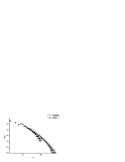
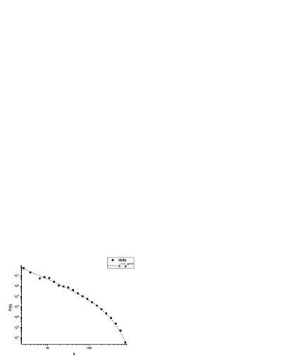
Figure 1: In the left panel we show the degree distribution for the Pythagorean network for $z<10^{4},10^{6}$. In the right panel we perform a logarithmic binning on the degree distribution for $z<10^{6}$ to illustrate the power law behaviour. The fitting curve is the power law with exponential cut-off in Eq.4.

To better understand how those structures form, we performed an $ageing$ analysis of the network. In Fig.2 we show the degree of the vertices versus their labels for different values of $z$. Small labels indicate old vertices. Peak values of the degree $k$ represent the major hubs of the network. For stochastic preferential growing networks [30], the high degree vertices are always the old vertices of the network. In the Pythagorean network this result does not hold. From Fig.2 we can see that after a while the old vertices’ degree freezes and hubs form between young and middle-aged vertices.

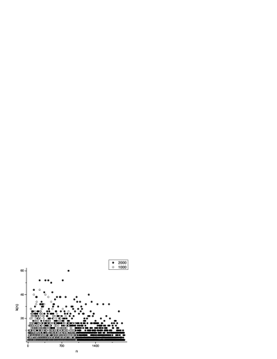
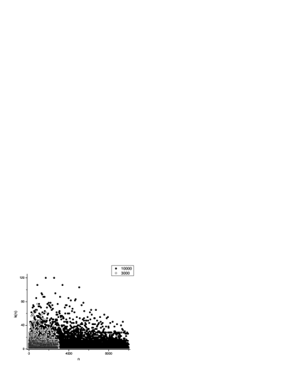
Figure 2: Representation of the aging of the hubs for the Pythagorean network for $z<1000,2000$ on the left and for $z<3000,10000$ on the right. $k$ is the degree of the vertices, while $n$ is their label. Small values of $n$ correspond to old vertices.

Since the Pythagorean network is made up of cliques it is interesting to look at its clustering coefficient.The clustering coefficient [1] is defined as

$$c(k_{i})=\frac{2e_{i}}{k_{i}(k_{i}-1)},$$ (5)

where $k_{i}$ is the degree of vertex $i$ and $e_{i}$ is the number of nearest neighbors of vertex $i$ that are connected to each other. We show in Fig.3 our measures of $c(k)$ on a Pythagorean network for different values of $z$. The regularity of the distribution is striking and due to the high regularity of the network. All vertices with $k=2$ form a triangle with their nearest neighbors, so that they have $c(k)=1$. The higher a vertex degree, the more improbable it is that its nearest neighbors are fully connected. Since for the inner geometry of the network $e_{i}\geq\frac{k_{i}}{2}$, it follows that $c(k_{i})\geq\frac{1}{k_{i}-1}$ and, obviously, $c(k_{i})\leq 1$. All the values of $c(k_{i})$ lie on well-determined levels defined by

$$c(k_{i})=\frac{k_{i}+2n}{k_{i}(k_{i}-1)},$$ (6)

where $n=0,1,2,...,n_{i}$ and $n_{i}=\frac{k_{i}(k_{i}-2)}{2}$. To demonstrate Eq.6 is a simple graphical exercise. Eq.6 is compared to the numerical simulation in Fig.3. For each $k_{i}$, the different values of $c(k_{i})$ are equally spaced at a distance of $\Delta(c(k_{i}))=\frac{2}{k_{i}(k_{i}-1)}$.

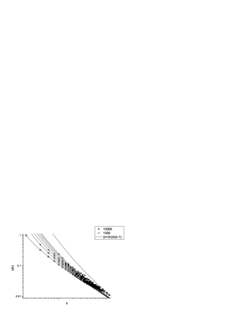
Figure 3: Clustering coefficient for the Phytagorean network measured in simulations with $z<1000,10000$. The lines represent Eq.6 for different values of $n$. In particular the greatest value of $n$ allowed for $z<10000$ is $n=23$.

Notice at last that, in contrast with the linear case, the network’s behaviour in the thermodynamic limit is now highly not trivial and probably cannot be described in detail before some open questions in number theory will be eventually answered. The numerical work we performed may however suggest some interesting conjectures. We think that the most relevant feature of our model is perhaps the ageing analysis showing that, when the network grows, the hubs are constantly rejuvenated, in sharp contrast with the behaviour of scale-free networks generated through the preferential attachment mechanism.

3 Model B

We now study the network generated by the deterministic rule expressed by the equation

$$x^{2}+y^{2}=z$$ (7)

This network is thus deeply connected with the classical Euler and Fermat Problem of finding all integers that can be expressed as the sum of two squares. In a sense this case is intermediate between the linear and the Pythagorean case. Notice, first of all, that in the thermodynamic limit Eq.7 generates a trivial network where each vertex’s degree goes to infinity. Indeed given any positive integer $x$, for any arbitrary integer $y$ (when $N\longrightarrow\infty$) we can always find an integer $z$ satisfying Eq.7. Thus we only need to consider the finite networks specified by the inequality $z<N$. The network attachment mechanism, as in Model A, will depend on the generating equation in the sense that every triple of integer numbers obeying Eq.7 forms a clique in the network.

The resulting network is very well connected since every couple of numbers at a certain time step (when $N$ is sufficiently large) forms a clique satisfying Eq.7. Nevertheless interesting topological properties emerge. In the left panel of Fig.4 we show the degree distribution for this network. The shape of the distribution is well approximated by a power law with exponent $-4.5$ for several decades of values of $k$. Very interestingly, after falling the distribution begins to rise again. On the right panel of the same figure we show the degree of the vertices against their label number $n$. This number can be considered as the birth time of the vertex so that we can observe the evolution of the hubs of the network with ageing. The degree is nearly constant and very high for small values of $n$ and it drops rapidly to small values for $n\sim\sqrt{N}$ (this comes from Eq.7, when $z\sim N$ then $x,y\sim\sqrt{N}$).

Notice that the power law exponent is considerably lower (at least from the point of view of network theory where power law exponents usually range between $-3$ and $-2$) than the one we recovered in the Pythagorean case. We interpret this weakening as the result of the upper thresholds we imposed to the network which, in this case, have a much stronger effect on the degree distribution than in the Pythagorean case.

In Fig.5 we show the clustering analysis for the network. On the left panel we show the clustering coefficient $c(k)$, defined in Eq.5, against the degree, while on the right panel we show the average clustering coefficient $<c(k)>$ against the degree. We can observe that it is very high for small values of $k$, where the degree distribution is a power law, then it is nearly constant for several decades and finally it falls rapidly to zero for high values of the degree. This behaviour has to do with the clique structure of the network. $c(k)=1$ as soon as isolated cliques form, that is for $k=2$, then its value falls as new connections are added and the degree increases.

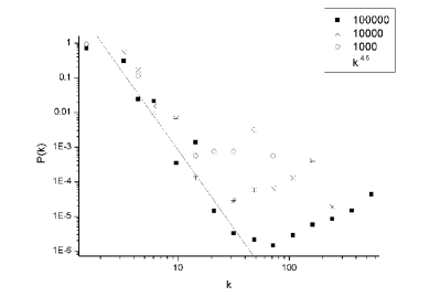
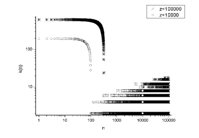
Figure 4: Left panel: degree distribution for the deterministic network generated by the rule in Eq.7 for $z<1000,10000,100000$. Right panel: representation of the aging of the hubs for the same network for $z<10000,100000$. $k$ is the degree of the vertices, while $n$ is their label. Small values of $n$ correspond to old vertices.

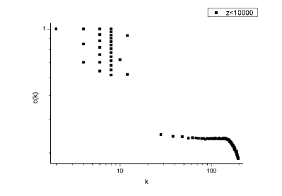
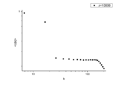
Figure 5: Left panel: clustering coefficient $c(k)$ against the degree $k$ for the deterministic network generated by the rule in Eq.7 for $z<10000$. Right panel: average clustering coefficient $c(k)$ against the degree $k$ for the deterministic network generated by the rule in Eq.7 for $z<10000$.

Conclusions

We have introduced the networks generated by Diophantine equations focusing on two classical problems of number theory widely studied since antiquity. We investigated first the Pythagorean problem of finding all triples of positive integers that can be represented geometrically as legs of a right-wristed triangle. We studied then the (closely related) problem of determining the set of positive integers that can be represented as the sum of two squares. These two questions, despite their apparent simplicity, have not yet been answered analytically in their full generality.

We noticed that these classical problems can be naturally translated into the language of network theory and studied them numerically in their finite versions (that is by not allowing integers to be greater than a fixed upper threshold). It is then easy to see that the equations considered generate clique structured networks, in an interesting analogy with many relevant real world networks such as social [31] and biological networks [22, 23].

In the Pythagorean case, where the network evolves through the deterministic attachment mechanism specified by Eq.3, we recovered a degree distribution consistent with a power law with exponential cut-off, in accordance with the behaviour displayed by many real world random networks [1].

We then performed an ageing analysis and showed that, in sharp contrast with stochastic preferential growing networks, hubs form between young and middle aged vertices (the degree of each vertex, after a while, freezes).

The power-law, in this case, is clearly not a by-product of any preferential attachment or fitness mechanism, but a consequence of the algebraic structure of Eq.3 itself. This shows once more that preferential attachment is a sufficient but not a necessary condition to the generation of scale-free topologies. As far as we are aware the network generated by Eq.3 is the first genuine example in literature of a deterministic scale-free network (at least in some approximation) which does not grow preferentially.

Power laws are normally regarded as a sign of complexity and we found it particularly stimulating to detect them not only in natural phenomena but also at the roots of number theory itself, indicating a fascinating connection between complex systems and pure mathematics. We then studied the second classical problem mentioned above studying the network generated by Eq.7 and recovered a degree distribution approaching a power-law with a relatively high exponent $\gamma\sim 4.5$ for several decades of values of $k$.

We believe that the study of networks generated by equations will turn out to represent an important field of interdisciplinary research and we hope that our discussion will be useful to researchers in both complex network theory and pure mathematics as a first step to recover more rigorous and general results. In particular, in future work it will be stimulating to investigate the relation between an equation’s algebraic properties (or analytic properties if, for instance, differential equations are considered) and the associated network’s topology.

Diophantine networks may find interesting theoretical and technological applications. First and foremost they can be used to design deterministic toy models of complex systems, allowing to find practical ways to build networks systematically without having to deal with different degrees of stochasticity in their architecture (in this sense they could play a role similar to the one played by the Euclidean grid in other traditional contexts). Diophantine networks may also allow to overcome some limitations intrinsic in the preferential attachment method, namely the fact that the hubs are usually the oldest vertices and never ”die”, leaving little room for network rejuvenation. Here instead we have a dynamic situation where hubs are dominant, during network growth, only for a limited period of time. There may be situations where this feature is realistic (for instance in models of technological developments). Another interesting application of the theory may be found in the study of the behaviour of dynamically evolving agents.

Acknowledgments

We thank the European Union Marie Curie Program (NET-ACE project, contract number MEST-CT-2004-006724) for financial support.

References

- [1] R.Albert, A.L.Barabási, Rev.Mod.Phys. 74, 47 (2002)
- [2] A.P.Masucci, G.J.Rodgers, Phys.Rev.E 74, 046115 (2006)
- [3] B.Bollobás, Random Graphs (Academic Press, London, 1985)
- [4] R.Pastor-Satorras, A.Vespignani, Scale-Free Networks (Wiley-VCH, Berlin, 2002), chapter Epidemics and Immunization
- [5] R.Albert, H.Jeong, A.L.Barabási, Nature 406, 378 (2000)
- [6] C.Bedogne’, G.J.Rodgers, Phys.Rev.E 74, 046115 (2006)
- [7] P.L.Krapivsky, S.Redner, F.Leyvraz, Phys.Rev.Lett. 85, 4629 (2000)
- [8] P.L.Krapivsky, S.Redner, Phys.Rev.E 63, 066123 (2001)
- [9] P.L.Krapivsky, G.J.Rodgers, S.Redner, Phys.Rev.Lett. 86, 5401 (2002)
- [10] V.D.P.Servedio, G.Caldarelli, Phys.Rev.E 70, 036126 (2004)
- [11] G.Caldarelli, A.Capocci, P.De Los Rios, M.A. Munoz, Phys.Rev.Lett. 89, 258702 (2002)
- [12] G.Ergun, G.J.Rodgers, Physica A 303, 261 (2002)
- [13] K.Austin, G.J.Rodgers, Proc.of the Int.Conf.of Comput.Science ICCS2004, 1087 (2004)
- [14] W.Hwang, P.L.Krapivsky, S.Redner, J.Math.Biol. 44, 375 (2002)
- [15] K.I.Goh, B.Kahng, D.Kim, Phys.Rev.Lett. 87, 278701 (2001)
- [16] Z.Zhang, F.Comellas, G.Fertin, L.Rong, J.Phys.A.Math.Gen. 39, 1811 (2006)
- [17] Z.Zhang, R.Lili, Z.Shuiseng, Phys.Rev.E 74, 046105 (2006)
- [18] J.S.Andrade Jr, H.Herrmann, R.F.S.Andrade, L.R.da Silva, Phys.Rev.Lett. 94, 018702 (2005)
- [19] R.F.SD.Andrade, J.G.V.Miranda, Physica A 356, 1 (2005)
- [20] T.Zhou,B.H.Wang, P.M.Hui, K.P.Chan, Physica A 367, 613 (2006)
- [21] K.Tokemoto, C.Oosawa, T.Akutsu, Physica A 380, 665 (2007)
- [22] R.Milo et al, Science 298, 824 (2002)
- [23] S.Shen-Orr, R.Milo, S.Mangan, U.Alam, Nat.Genet.31, 64 (2002)
- [24] G.Ghoshal, M.E.J.Newman, arXiv:physics/0608057v2 (2007)
- [25] A.Ivic et al, arXiv:math.NT/0410522v1 (2004)
- [26] E.K.Hinson, Fibonacci Quart. 30, 335 (1992)
- [27] M. Benito, J.L.Varona, J. of Comput. and Appl.Math. 143, 117 (2002)
- [28] F.Wiedijk, Formalized Mathematics 9, 809 (2001)
- [29] M. Kuehleitner, Abh.Math.Semin.Univ.Hamb. 63, 105 (1993)
- [30] J.Lambek, L.Moser, Pacific J.Math. 5, 73 (1955)
- [31] J.Scotts, Social Network Analysis: A Handbook, 2nd Ed. Newberry Park, CA: Sage (2000)
- [32] D.J.Watts, P.J.Dodds, M.E.Newman, Science 296, 1302 (2002)
- [33] G.Palla, I.Derény, I.Farkas, T.Vicsek, Nature 435, 207 (2005)
- [34] T.S.Evans, arXiv:0711.0603v1 (2007)