A simple method for timing an XFEL source to high-power lasers

Abstract

We propose a technique, to be used for time-resolved pump-probe experiments, for timing an x-ray free electron laser (XFEL) to a high-power conventional laser with femtosecond accuracy. Our method takes advantage of the same electron bunch to produce both an XFEL pulse and an ultrashort optical pulse with the help of an optical radiator downstream of the x-ray undulator. Since both pulses are produced by the same electron bunch, they are perfectly synchronized. Application of cross-correlation techniques will allow to determine relative jitter between the optical pulse (and, thus, the XFEL pulse) and a pulse from an external pump-laser with femtosecond resolution. Technical realization of the proposed timing scheme uses an optical replica synthesizer (ORS) setup to be installed after the final bunch-compression stage of the XFEL. The electron bunch is modulated in the ORS setup by an external optical laser. Subsequently, it travels through the main undulator, and produces the XFEL pulse. Finally, a powerful optical pulse of coherent edge radiation is generated as the bunch passes through a long straight section and a separation magnet downstream of the main undulator. Our study shows that at a moderate (about $10\%$) density modulation of the electron bunch at the location of the optical radiator allows production of high power x-ray and optical pulses. Relative synchronization of these pulses is preserved by using the same mechanical support for both x-ray and optical elements transporting radiation down to the experimental area, where single-shot cross-correlation between optical pulse and pump-laser pulse is performed. We illustrate the potential of the proposed timing technique with numerical examples referring to the European XFEL facility.

1 Introduction

Time-resolved experiments are used to monitor time-dependent phenomena. In typical pump-probe experiments a short probe pulse follows a short pump pulse at some specific delay. Femtosecond capabilities have been available for some years at visible wavelengths Zewail . However, there is a strong interest in extending these techniques to x-ray wavelengths, where one could directly probe structural changes with atomic resolution. This goal will be achieved with the realization of x-ray free electron lasers (XFELs) XFEL , SLAC , SCSS . In their initial configurations, XFELs will produce radiation pulses with duration of about a hundred femtosecond, which will allow time-resolved studies of transient structures of matter on the time-scale of chemical reactions.

One of the main technical problems for the realization of pump-probe experiments is the relative synchronization of radiation pulses from XFEL and optical laser. Both x-ray and optical pulses are subject to time-jitter. In an XFEL, radiation is produced by an electron bunch travelling through an undulator. The budget for time jitter of the electron bunch starts to accumulate from the photo-injector laser system. Extra source of jitter is constituted by fluctuations of the electron energy, which transform to time jitter in magnetic bunch-compressors. The pump-laser itself has an intrinsic time jitter caused e.g. by mechanical vibrations in the laser oscillator or electrical-noise in the stabilization electronics.

There exists a tendency for straightforward solution of the problem by means of implementation of a precise synchronization system at XFELs, aiming all clocks and triggers within the facility to be perfectly synchronized GS1 , GS2 , GS3 . Once this is done, temporal resolution of pump-probe experiment will be defined by the synchronization system plus intrinsic time-jitter of the pump-laser system. However, precise synchronization on a kilometer-scale facility is a rather challenging task, and it is not clear, at the moment, what will be the overall practical accuracy limit for the synchronization of XFEL pulses to pulses from external lasers.

Approaches based on generation of two coherent radiation pulses of different colors by the same electron bunch passing through two distinct insertion devices have been proposed in TC1 , TC2 . Intrinsic feature of these schemes is an ideal mutual synchronization of the radiation pulses. With careful design of the optical transport system from source to sample it is possible to reach femtosecond level of synchronization. One of the schemes, using far infrared and VUV radiation pulses is being experimentally realized at FLASH, the free-electron laser in Hamburg fir-pp .

Recently, an alternative concept has been proposed for realization of pump-probe experiments with XFEL pulses and powerful optical pulses from external lasers BILL , fel07-TUPPH013 . The basic idea is to shift the attention from the problem of absolute synchronization to the problem of measurement of relative jitter between x-ray and optical pulses. If a relative delay is known for each pump-probe event, a sorting of results according to measured delay times gives the required experimental outcome. In this paper we propose a concept of time-arrival monitor allowing measurement of a relative delay between XFEL and optical pulses on a femtosecond time scale. Our scheme makes use of the same electron bunch to produce both an XFEL pulse and a powerful laser-like (bandwidth-limited and diffraction-limited) optical pulse. The latter is generated downstream of the x-ray undulator, and will be naturally synchronized to the XFEL pulse. Relative synchronization is preserved by using the same mechanical support for optical elements transporting x-ray pulse and optical pulse down to the experimental area. There, single-shot cross-correlation between the optical pulse and the pump-laser pulse can be performed yielding, effectively, the temporal delay between XFEL pulse and pump-laser pulse.

Implementation of the proposed scheme for pump-probe experiments into the project of the European XFEL XFEL is described in detail. We show that it naturally fits into the project. A modulation at optical frequency is imprinted onto the electron bunch using the optical replica synthesizer (ORS) setup ORS1 that will be installed after the final beam compression stage at the energy of 2 GeV. Subsequently, electrons travel through the main undulator and radiate the XFEL pulse. Finally, the presence of a long straight section and a separation magnet downstream of the main undulator serve as optical radiator, where the modulated electron bunch produces a powerful pulse of coherent edge-radiation.

The proposed arrival-time monitor can be realized without the addition of specific hardware in the accelerator and undulator tunnels, and requires minimal efforts. The applicability of the present scheme is not restricted to the European XFEL setup. Other projects, e.g. the LCLS or SCSS facility SLAC , SCSS , may benefit from our proposal too.

2 Timing system description

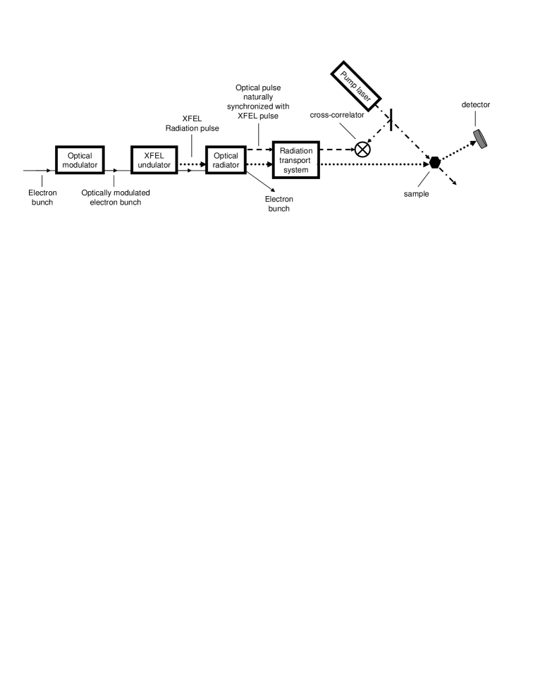
Figure 1: Scheme for pump-probe experiments with XFEL pulses and pulses produced by an external laser. Operation of the scheme is based on production by the electron bunch of an optical pulse naturally synchronized with the XFEL pulse. Relative synchronization is preserved by using the same radiation transport system to the experimental area. The optical pulse is then used to monitor the delay time between pump and probe by correlating it with the pump laser.

A basic scheme of the timing system is shown in Fig. 1. Discussions in this paper focus on design and parameters (see Fig. 2) of the SASE 1 line of the European XFEL, operating in the wavelength range around $0.1$ nm. Main elements of the timing system are energy modulator (constituted by seed laser and undulator modulator), dispersion section and radiator.

The energy modulator (see Fig. 3) is located after the second bunch compressor (BC2), where the electron energy is about $2$ GeV. A laser pulse at wavelength $\lambda=400$ nm is used to modulate the electron energy at the same wavelength. The duration of the laser pulse is chosen to be about $1$ ps, much longer than the time-jitter of the electron pulse (a fraction of a picosecond) to avoid synchronization problems. The energy of the laser pulse is about $0.5$ mJ. Laser beam is focused onto the electron beam in a short modulator undulator, with a number of periods $N_{w}=5$, resonant at the seed laser wavelength $\lambda=400$ nm. Energy modulation with an amplitude of about $0.5$ MeV is achieved due to interaction with the electron bunch in the modulator undulator. Subsequently, the electron bunch passes through the dispersion section with momentum compaction $R_{56}\simeq 15\mu$m, where the energy modulation induces a density modulation at the seed-laser wavelength. With parameters discussed above, the density modulation reaches an amplitude of about $5\%$. Following the dispersion section the bunch is accelerated up to the energy of $17.5$ GeV in the main accelerator, it passes trough the collimator system and is directed to the SASE 1 x-ray undulator.

A high-current (5 kA) electron beam is transported through the XFEL linac, and it is therefore mandatory to include self-interaction effects in our analysis. During the passage of the bunch through the accelerator, the initial density modulation produces an energy modulation due to longitudinal impedance caused by space-charge fields. If the collimation system is properly tuned, such energy modulation can induce further modulation in density. Calculations presented in Section 3 show that exploitation of self-interaction mechanisms allow one to deliver, at the entrance of the SASE 1 undulator, an electron bunch with a $10\%$ density modulation, and negligible energy modulation.

The SASE FEL process in the baseline undulator is not perturbed by such level of density modulation: fluctuations of the electron current density serve as input signal for the radiation amplification process, which develops nearly in the same way as with an unmodulated electron bunch. As a result, at the exit of the SASE 1 undulator the electron bunch produces the nominal x-ray pulse.

Finally, after the SASE 1 undulator, the modulated electron bunch passes through a long straight section followed by a separation magnet, which separates the electron bunch from the SASE pulse. Due to the presence of the combination of straight section and separation magnet, the electron bunch emits an optical pulse of coherent edge radiation at the wavelength of the bunch density modulation. Such an optical pulse carries about $10^{12}$ photons (order of a microjoule) and is delivered in a bandwidth-limited and diffraction-limited pulse.

Summing up, combination of an optical modulator after magnetic bunch compressor BC2 and optical radiator after the baseline undulator will allow to produce a powerful laser-like optical pulse at the entrance of the photon beamline. This laser-like pulse is naturally synchronized with the electron bunch and thereby with the x-ray pulse. Thus, the problem of measuring the time-shift between a pump-laser pulse and a (x-ray) probe pulse is reduced to the problem of measuring the time delay between two ultrashort optical pulses, which may be solved with standard techniques.

Contrarily to the x-ray pulse, which is peaked on-axis, the edge-radiation pulse is peaked in the forward direction at an angle of a few tens of microradians. The distance from the separation magnet to the first (x-ray) mirror station is about $300$ m. According to calculations presented in Section 4, the diameter of the spatial distribution of edge radiation at this distance will be about $3$ cm, which fits with the aperture of the photon beamline.

Relative synchronization of x-ray and optical pulses must be preserved during propagation to the experimental area. The best way to do so is to use the same mechanical support for both optical elements transporting the x-ray pulse and optical elements transporting the optical pulse. For example, optical elements for the transportation of edge-radiation may be directly assembled on the x-ray mirrors. After passing through the transport system, the edge-radiation pulse will reach the experimental area, where a single-shot cross-correlation measurement with the pump-laser pulse can be performed. In reference CROS the possibility of extracting the temporal shift between pulses from two ultrashort laser pulses was experimentally demonstrated. The method was based on sum-frequency generation in a non-linear crystal. The intrinsic accuracy of this technique was shown to be within the femtosecond range. Successful measurements of the time-offset signal were performed even when one of the two pulses was very weak (down to $10^{6}$ photons per pulse).

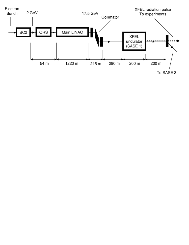
Figure 2: Integration of the time-arrival monitor in the European XFEL setup makes use of the Optical Replica Synthesizer (ORS). The ORS is used to imprint density modulation onto electron beam. Optical radiator is the combination of straight-section and separation magnet after the SASE 1 undulator which produsese powerful optical pulse of coherent edge radiation.

3 Operation of the optical modulator

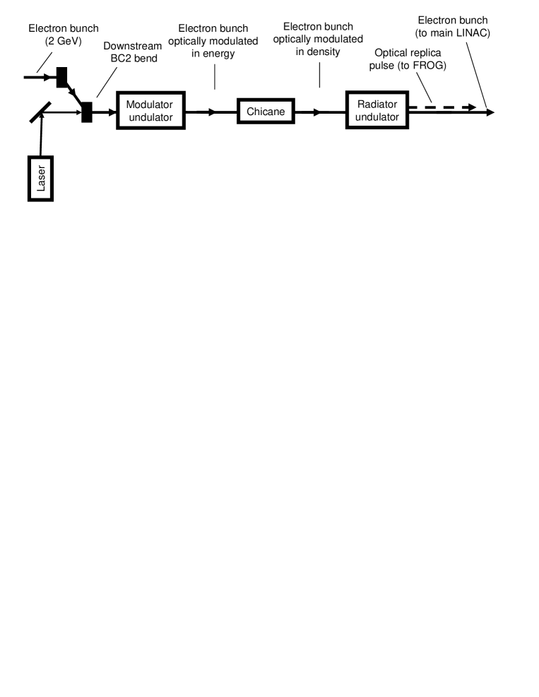
Figure 3: The Optical Replica Synthesizer (ORS) will be used to superimpose density modulation at optical wavelength on the electron bunch. First, energy modulation is created by letting a laser interact with the bunch inside a modulation undulator. Second, a dispersion section (magnetic chicane) induces the desired density modulation. The radiator undulator, used in optical-replica ultrashort electron bunch diagnostics, is switched off during operation of the arrival-time monitor.

The modulator to be used in our scheme is the optical replica modulator ORS1 , which consists of three elements (see Fig. 3): an optical seed laser, a modulator undulator and a dispersion section (magnetic chicane). The radiator undulator shown in Fig. 3, used in optical-replica ultrashort electron bunch diagnostics, is switched off during operation of the arrival-time monitor. The seed laser pulse interacts with the electron beam in the modulator undulator, which is resonant with the laser wavelength $\lambda$. As a result, the electron bunch is modulated in energy. In the following dispersion section the energy modulation induces a density modulation at the optical wavelength.

The dispersion section is designed to produce an energy dependence of the particles path length $\delta z=R_{56}\delta\gamma/\gamma_{0}$, where $\delta\gamma$ is the energy deviation of a particle in units of the rest mass, $\delta z$ is the deviation from the path length of an electron with nominal energy $\gamma_{0}$ in units of the rest mass, and $R_{56}$ is the compaction factor of the dispersion section. $\delta\gamma$ and $\delta z$ may assume positive or negative values, while $R_{56}>0$, the dispersion section being a chicane. Suppose that at the entrance of the chicane we have an initial energy modulation. Then, in units of the rest mass, the energy deviation of each particle due to this energy modulation is given by $(\Delta\gamma)_{i}\sin(\psi)$, where $\psi=\omega[z/v_{z}(\gamma_{0})-t]$ is the modulation phase, with $v_{z}$ the longitudinal velocity of a nominal electron, and $\omega=2\pi c/\lambda$, $c$ being the speed of light in vacuum. Here $(\Delta\gamma)_{i}$ is the amplitude of our small ($|(\Delta\gamma)_{i}|/\gamma_{0}\ll 1$) energy modulation taken with its own sign. At the exit of the chicane we may express the current as $I=I_{0}[1+a_{i}\cos(\psi)]$. Here $I_{0}$ is the unmodulated electron beam current, and $a_{i}$ is the amplitude of our small ($|a_{i}|\ll 1$) density modulation, also taken with its own sign.

Neglecting collective effects, the amplitude of density modulation at the exit of the chicane, $a_{i}$, approaches Czonka

$$a_{i}=\frac{R_{56}}{\lambdabar}\frac{(\Delta\gamma)_{i}}{\gamma_{0}}\exp\left[-\frac{1}{2}\frac{\left\langle(\delta\gamma)^{2}\right\rangle}{\gamma_{0}^{2}}\frac{R_{56}^{2}}{\lambdabar^{2}}\right]~{},$$ (1)

where $\left\langle(\delta\gamma)^{2}\right\rangle^{1/2}$ is the rms uncorrelated energy spread of the electron bunch in units of the rest mass, and $\lambdabar=\lambda/(2\pi)$ is the reduced modulation wavelength. In the case of the European XFEL (see XFEL , Fig. 2 and Fig. 3) $\gamma_{0}\simeq 4\cdot 10^{3}$, corresponding to an energy of $2$ GeV, $\left\langle(\delta\gamma)^{2}\right\rangle^{1/2}\simeq 2$, corresponding to $1$ MeV rms uncorrelated energy spread, $(\Delta\gamma)_{i}\simeq 1$, corresponding to $0.5$ MeV modulation, and $\lambda=400$ nm, corresponding to the second harmonic of a Ti:Si laser. A value $R_{56}\simeq 30\mu$m leads to a modulation amplitude $a_{i}\simeq 0.1$. Note that in this case the exponential suppression factor in Eq. (1) is about $0.98$, and can be practically neglected.

If collective effects could be neglected during the transport of the bunch, one could propagate the $10\%$ initial density modulation up to the radiator, accounting for velocity bunching and, possibly, for the presence of a non-zero compaction factor at the collimation section $R^{(c)}_{56}$. In this case, estimations would remain within the framework of single-particle dynamics. Tuning the energy in the optical seed laser pulse, one may easily achieve a final modulation $a_{f}=0.1$ at the optical radiator entrance.

However, collective effects strongly influence the modulation process in our jitter-monitoring scheme. In other words, the problem of propagation of the induced beam density modulation through the setup depicted in Fig. 2 is a problem involving self-interactions. As the bunch progresses through the linac, the modulation of the bunch density produces an energy modulation due to longitudinal impedance caused by space-charge field. This process is complicated by the fact that, due to the presence of energy and density modulation, plasma oscillations can develop. One should account for these facts in order to quantify energy and density modulation before the collimation section. Then, in the collimation section, the energy modulation induces extra-density modulation due to non-zero compaction factor. Finally, longitudinal space-charge impedance is responsible for further energy modulation and further plasma oscillations during the passage of the beam in the main undulator. As a result, the initial beam modulation, in energy and density, will be modified by the passage through the setup. In order to study the feasibility of our scheme one needs to estimate what modifications will take place.

At the entrance of the accelerator, the density modulation amplitude is given by $a_{i}$, and the energy modulation amplitude by $(\Delta\gamma)_{i}$. Due to energy modulation, particles undergo a phase shift, with respect to the phase $\psi$, which is responsible for a change in the density modulation along the acceleration section. Also the energy modulation is a varying function of $z$ because of the presence of longitudinal space-charge forces. Indicating with $a(z)$ and with $\Delta\gamma(z)$ the density and energy modulation amplitudes along the accelerator we may write

$$\frac{da}{dz}=\frac{1}{\lambdabar}\frac{\Delta\gamma(z)}{\gamma^{3}(z)}~{},$$ (2)

where, additionally, the relativistic Lorentz factor of the bunch, $\gamma(z)$, accounts for the acceleration process. Eq. (2) can be directly derived from Eq. (1) substituting $a_{i}$ and $(\Delta\gamma)_{i}$ with $a(z)$, and $\Delta\gamma(z)$, neglecting the exponential suppression factor due to uncorrelated energy spread, remembering that the compaction factor for a free-space section of length $\delta z$ is given by $R_{56}=\delta z/(\lambdabar\gamma^{2})$, and taking the limit for $\delta z\longrightarrow 0$.

One can estimate the derivative of $\Delta\gamma(z)$ along the XFEL linac using results from papers studying microbunching instabilities like LSCF . We can write:

$$\frac{d(\Delta\gamma)}{dz}=-\frac{4\pi}{Z_{0}}a(z)\frac{I_{0}}{I_{A}}\frac{d|Z|}{dz}~{},$$ (3)

where $Z(z,\omega)$ is the longitudinal impedance induced by space charge, $Z_{0}$ is the free-space impedance, expressed in the same units of $Z$, and $I_{A}\simeq 17$ kA the Alfven current.

The longitudinal impedance induced by space charge in free space was studied in the case of an electron bunch with finite transverse profile in ROSE , LWF1 . In that reference we gave analytical expressions for the impedance in the steady state limit, which can be easily generalized in the case of adiabatic acceleration, when $\lambdabar(d\gamma^{2}/dz)=2\lambdabar\gamma(d\gamma/dz)\ll 1$. The adiabatic acceleration limit can always be used in our case. Assuming a constant acceleration gradient $d\gamma/dz\equiv g\simeq 25\mathrm{m}^{-1}$ (see XFEL ), we have $2\lambdabar\gamma(d\gamma/dz)\simeq 0.01$ for $\gamma=4\cdot 10^{3}$, corresponding to the lowest energy of $2$ GeV, and $2\lambdabar\gamma(d\gamma/dz)\simeq 0.1$ for $\gamma=3.5\cdot 10^{4}$, corresponding to the highest energy of $17.5$ GeV, whereas the largest effects due to longitudinal impedance are expected in the first part of the acceleration process. Then, using results in LWF1 , which are valid for a Gaussian transverse distribution of the electron bunch, we find that Eq. (3) can be written as

$$\frac{d(\Delta\gamma)}{dz}\simeq-\frac{a(z)}{\lambdabar(\gamma_{0}+gz)^{2}}\frac{I_{0}}{I_{A}}{\exp\left[\frac{\epsilon_{n}\beta}{(\gamma_{0}+gz)^{3}\lambdabar^{2}}\right]~{}\Gamma\left[0,\frac{\epsilon_{n}\beta}{(\gamma_{0}+gz)^{3}\lambdabar^{2}}\right]}~{}.$$ (4)

Here $\Gamma$ is the incomplete gamma function, $\beta$ is the average betatron function in the accelerator, and $\epsilon_{n}$ is the normalized emittance.

The system of coupled differential equations constituted by Eq. (2) and Eq. (4) should be solved with given initial conditions $a(0)=a_{i}$ and $\Delta\gamma(0)=(\Delta\gamma)_{i}$ at the entrance of the accelerator in order to obtain density and energy modulation at the entrance of the collimator. Such system of equations accounts for plasma oscillations of the electron bunch in the limit for adiabatic acceleration, with the help of a longitudinal impedance averaged along the transverse direction. A more detailed analysis of space-charge waves performed as a function of the transverse coordinates (i.e. without averaging the longitudinal impedance) is given in SCTH , where we studied the problem of plasma oscillations for an electron bunch with arbitrary transverse profile going along a straight section with uniform motion.

We assume an average betatron function of about $\beta=25$ m along the main accelerator and a normalized emittance $\epsilon_{n}=1.4$ mm$\cdot$mrad (see XFEL ). Setting the acceleration length $d_{a}\simeq 1220$ m (see Fig. 2) and $I_{0}\simeq 5$ kA, numerical analysis shows that our initial conditions $a_{i}\simeq 0.05$ and $(\Delta\gamma)_{i}\simeq 1$ yield, at the entrance of the collimator $z=d_{c}$, $a(d_{c})\simeq 0.03$ and $\Delta\gamma(d_{c})\simeq-6$.

The nominal value of the compaction factor of the collimator $R^{(c)}_{56}$ is set to zero, with possibility of fine tuning around this value of about $\pm 100~{}\mu$m. Taking advantage of this possibility and setting $R^{(c)}_{56}\simeq+50\mu$m, at the exit of the collimator one obtains a density modulation $a_{c}\simeq-0.1$, whereas the energy modulation remains unvaried $(\Delta\gamma)_{c}\simeq-6$.

Further on, energy and density modulation should be propagated through a straight section followed by the main XFEL undulator. Propagation can be performed using the same set of equations Eq. (2) and Eq. (4), setting $g=0$, using an energy of $17.5$ GeV and an average value of the betatron function $\beta=20$m. This gives only a correction to the energy modulation, so that at the entrance of the XFEL undulator, at $z=d_{u}$, one still has $a(d_{u})\simeq-0.1$, while $\Delta\gamma(d_{u})\simeq-5$. Decrease of the energy modulation is related to an advantageous initial phase of plasma oscillation at the entrance of the straight section. Numerical analysis shows that such an energy modulation, being smaller than the foreseen XFEL spectral bandwidth $0.08\%$ XFEL , will not alter the XFEL process (see Figs. 5 and 5).

Figure 4: Dependence of the FEL output power on the energy modulation for undulator SASE 1 at the European XFEL XFEL . Amplitude and period of electron bunch modulation are 10% and 400 nm, respectively. Radiation power is normalized to saturation power for an unperturbed bunch. Simulations have been performed with the code FAST FAST .

Figure 5: Normalized spectrum of the FEL radiation pulse at zero energy modulation (left plot), and at $\Delta\gamma mc^{2}=4$ Mev (right plot). Numerical example corresponds to undulator SASE 1 at the European XFEL XFEL . Amplitude and period of electron bunch modulation are 10% and 400 nm, respectively. Simulations have been performed with the code FAST FAST .

Similarly as before, the passage in the main XFEL undulator has the effect of decreasing the energy modulation level, too. Moreover, although the undulator is shorter than the straight section preceding it, the effect on the energy modulation is stronger. In fact, the longitudinal Lorentz factor $\gamma_{z}=\gamma/\sqrt{1+K^{2}/2}$ should be used in the undulator instead of $\gamma$ (see reference OURX ). Since $K=3.3$, $\gamma^{2}$ and $\gamma_{z}^{2}$ differ of about an order of magnitude, hence the different influence of the undulator compared with the straight section. In the undulator, Eq. (2) and Eq. (4) are modified to

$$\frac{da_{i}}{dz}=\frac{1}{\lambdabar}\frac{\Delta\gamma}{\gamma\gamma_{z}^{2}}~{},$$ (5)

and

$$\frac{d\Delta\gamma}{dz}\simeq-\frac{a_{i}(z)}{\lambdabar\gamma_{z}^{2}}\frac{I_{0}}{I_{A}}{\exp\left[\frac{\epsilon_{n}\beta}{\lambdabar^{2}\gamma_{0}\gamma_{z}^{2}}\right]~{}\Gamma\left[0,\frac{\epsilon_{n}\beta}{\lambdabar^{2}\gamma_{0}\gamma_{z}^{2}}\right]}~{}.$$ (6)

Solving numerically with previously found initial conditions $a(d_{u})$ and $\Delta\gamma(d_{u})$, and using $\beta=40$m, one finds the energy and density modulation levels at the radiator entrance, $a_{f}\simeq-0.1$ and $(\Delta\gamma)_{f}\simeq-2$.

As a final remark it should be noted that, pending design finalization, the $R^{(c)}_{56}$ value may be set to any value from $-1$ mm to $+1$ mm, different from the nominal value $R^{(c)}_{56}=0$. Depending on this value and, possibly, using the fine tuning option to increase or decrease the $R^{(c)}_{56}$ value up to $\pm 100\mu$m, different initial conditions should be set to obtain acceptable values for $a_{f}$ and $(\Delta\gamma)_{f}$. For example, if $R^{(c)}_{56}=+1$ mm, setting $a_{i}=0$ and $(\Delta\gamma)_{i}\simeq 0.3$ (corresponding to about $0.15$ MeV) would yield $a_{f}\simeq-0.1$ and $(\Delta\gamma)_{f}\simeq 6$, corresponding to about $3$ MeV energy modulation, which is perfectly compatible with our scheme.

It follows that the optical modulator can induce about $10\%$ density modulation at the entrance of the optical radiator, $|a_{f}|\simeq 0.1$, and acceptable energy modulation, independently of the design of the collimation section, without perturbation of the FEL process in the baseline undulator.

4 Operation of the optical radiator

After collimation we deal with an electron bunch modulated in density at optical wavelength. This wavelength is much larger than the geometrical emittance of the beam, and in our case the electron bunch can be considered as a filament with no transverse dimension nor divergence, as far as optical wavelengths are concerned. An analysis of the problem in the space-frequency domain ARTF shows that when a filament beam modulated in density passes through a given trajectory, it produces coherent radiation very much likely a single electron. In general, one needs to solve Maxwell’s equation for given macroscopic sources. A paraxial treatment is possible, based on the ultrarelativistic assumption $1/\gamma^{2}\ll 1$. Consider the transverse components of the Fourier transform of the electric field. They form a vector $\vec{\bar{E}}(\vec{r},z)$, dependent on transverse and longitudinal coordinates $\vec{r}$ and $z$. From the paraxial approximation follows that the envelope $\vec{\widetilde{E}}=\vec{\bar{E}}\exp{[-iz/\lambdabar]}$, does not vary much along $z$ on the scale of the reduced wavelength $\lambdabar$. With some abuse of language we will indicate $\vec{\widetilde{E}}$ as ”the field”. The field obeys the following paraxial wave equation in the space-frequency domain: $\mathcal{D}\left[\vec{\widetilde{E}}(z,\vec{r},\omega)\right]=\vec{g}(z,\vec{r},\omega)$. Here $\omega=2\pi c/\lambda$, and the differential operator $\mathcal{D}$ is defined by $\mathcal{D}\equiv\left({\nabla_{\bot}}^{2}+{2i\omega/{c}}\cdot{\partial_{z}}\right)$, ${\nabla_{\bot}}^{2}$ being the Laplacian operator over transverse cartesian coordinates. The source-term vector $\vec{g}(z,\vec{r})$ is specified by the trajectory of the source electrons, and can be written in terms of the Fourier transform of the transverse current density, $\vec{\bar{j}}(z,\vec{r},\omega)$, and of the charge density, $\bar{\rho}(z,\vec{r},\omega)$, as $\vec{g}=-{4\pi}\exp\left[-{i\omega z}/{c}\right]\left({i\omega}/{c^{2}}\cdot\vec{\bar{j}}-\vec{\nabla}_{\bot}\bar{\rho}\right)$. Vector $\vec{\bar{j}}$ and $\bar{\rho}$ are regarded as given data. In this paper we will treat $\vec{\bar{j}}_{\bot}$ and $\bar{\rho}$ as macroscopic quantities, without investigating individual electron contributions.

From the previous discussion it follows that, as concerns emission of coherent optical radiation, our setup reduces to an upstream bending magnet (corresponding to the last bend of the collimator) followed by a straight section, an undulator (the main SASE 1 undulator), a second straight section and a downstream separation bending magnet, which divides the electron beam from the XFEL pulse (see Fig. 2). We picture the upstream bending magnet as a ”switch-on” of both harmonics of the electromagnetic sources and of the field. Similarly, the downstream bend enforces a ”switch-off” process.

When a modulated beam passes through a straight section limited by upstream and downstream bending magnets, it produces edge radiation (see among others, BOSF , CHUN and references therein). In our case, trajectory from the collimator section up to the beam dump is more complicated than a single straight section limited by bending magnets, but conceptually the mechanism of radiation production is the same. Moreover, the influence of bending magnet radiation to the field contribution can be shown to be negligible. To see this, it is sufficient to compare the radiation formation length of the field associated with bending magnets with the radiation formation length of the shortest straight section. Deflection introduced in the collimation section corresponds to a bending radius of $400$ m. Deflection introduced between SASE 1 and SASE 3 corresponds, instead, to a bending radius of about $200$ m. For a wavelength $\lambda=400$ nm and bending radius $R=400$ m we obtain the longest formation length $(\lambdabar R^{2})^{1/3}\simeq 0.2$ m. For the shortest straight section of length $L=200$ m, the edge-radiation formation length would be $\min[L,2\gamma^{2}\lambdabar]=2\gamma^{2}\lambdabar\simeq 150$ m, which is about $10^{3}$ times longer than the formation length for the bends. It follows that field contributions from bending magnets can be neglected with an accuracy $10^{-3}$, and a sharp-edge approximation applies.

Understanding the operation of the optical radiator is made simpler with the help of the theoretical study in reference OURF . In that reference we showed that radiation from an ultra-relativistic filament beam along the trajectory specified above can be interpreted as radiation from three virtual sources, located at specific longitudinal positions. Specification of these virtual sources amounts to specification of three field distributions $\vec{\bar{E}}(\vec{r},z_{s})$ at three distinct locations $z_{s}$. In principle these locations are a matter of taste, but there are particular choices of $z_{s}$ where $\vec{\bar{E}}(\vec{r},z_{s})$ exhibit plane wavefronts and are similar to waists of laser beams. In the case under study these privileged longitudinal positions are the center of the straight sections and the center of the undulator. Let us indicate with $L_{1}$ and $L_{2}$ the lengths of upstream and downstream straight sections, with $L_{w}$ the length of the main XFEL undulator and set $z=0$ in its center. In this case, the three sources are located at $z_{s1}=-(L_{w}+L_{1})/2$, $z_{s2}=0$ and $z_{s3}=(L_{w}+L_{2})/2$. Since the virtual sources exhibit plane wavefronts, they are completely specified by real-valued amplitude distributions of the field. In the case of a single electron, these were derived from the far zone field distribution and were found to be OURF :

$$\vec{\widetilde{E}}_{1}\left(z_{s1},\vec{r}\right) =-\exp\left[-\frac{i}{4}\left(\frac{L_{w}}{\gamma_{z}^{2}\lambdabar}+\frac{L_{1}}{\gamma^{2}\lambdabar}\right)\right]$$ (8)

$$\times\frac{eL_{1}}{2\pi c\lambdabar^{2}}\int d\vec{\theta}~{}\vec{\theta}~{}\mathrm{sinc}\left[\frac{1}{4}\left(\frac{L_{1}\theta^{2}}{\lambdabar}+\frac{L_{1}}{\gamma^{2}\lambdabar}\right)\right]\exp\left[\frac{i}{\lambdabar}\vec{r}\cdot\vec{\theta}\right]~{},$$

$$\vec{\widetilde{E}}_{2}(z_{s2},\vec{r}) = -\frac{eL_{w}}{2\pi c\lambdabar^{2}}\int d\vec{\theta}~{}\vec{\theta}~{}\mathrm{sinc}\left[\frac{1}{4}\left(\frac{L_{w}\theta^{2}}{\lambdabar}+\frac{L_{w}}{\gamma_{z}^{2}\lambdabar}\right)\right]\exp\left[\frac{i}{\lambdabar}\vec{r}\cdot\vec{\theta}\right]~{}$$ (9)

and

$$\vec{\widetilde{E}}_{3}\left(z_{s3},\vec{r}\right) =-\exp\left[\frac{i}{4}\left(\frac{L_{w}}{\lambdabar\gamma_{z}^{2}}+\frac{L_{2}}{\gamma^{2}\lambdabar}\right)\right]$$ (12)

$$\times\frac{eL_{2}}{2\pi c\lambdabar^{2}}\int d\vec{\theta}~{}\vec{\theta}~{}\mathrm{sinc}\left[\frac{1}{4}\left(\frac{L_{2}\theta^{2}}{\lambdabar}+\frac{L_{2}}{\gamma^{2}\lambdabar}\right)\right]\exp\left[\frac{i}{\lambdabar}\vec{r}\cdot\vec{\theta}\right]~{}.$$

Note that the field is radially polarized. Aside for a different phase, Eq. (8), Eq. (LABEL:vir1ebf) and Eq. (12) have a similar mathematical structure. However, for SASE 1, $K=3.3$, so that $\gamma_{z}^{2}=\gamma^{2}/(1+K^{2}/2)$ is about an order of magnitude smaller than $\gamma^{2}$. It follows that the second term in the $\mathrm{sinc}(\cdot)$ function of Eq. (8) or Eq. (12) is much smaller than the analogous term in Eq. (LABEL:vir1ebf). In particular, for our study case we have ${L_{1}}/({4\lambdabar\gamma^{2}})=0.97$ and ${L_{2}}/({4\lambdabar\gamma^{2}})=0.67$ of order unity, but ${L_{w}}/({4\lambdabar\gamma_{z}^{2}})=4.3$. As a result, the $\mathrm{sinc}(\cdot)$ function in Eq. (12) is strongly suppressed, one may neglect the virtual source located in the center of the undulator and let $\vec{\widetilde{E}}_{2}(z_{s2},\vec{r})=0$, at least in first approximation. It should be remarked that the virtual source $\vec{\widetilde{E}}_{2}$ is responsible for a field contribution known as transition undulator radiation. Typical expressions for TUR emission KIM1 , KINC , CAST consist of relations for the energy distribution of radiation in the far zone that account for the presence of the virtual source at $z_{s2}$ alone, without considering further contributions due to other elements in the beamline, e.g. the straight sections in our case. As it was shown in BOS4 and OURF these expressions have no physical meaning. In our study case, as we have just seen, the contribution from transition undulator radiation can be even neglected.

We are thus left with the contributions from two virtual sources located at $z_{s1}$ and $z_{s3}$, accounting for edge radiation emission from the straight lines before and after the undulator. However, the contribution from the upstream straight section will be strongly suppressed by a photon stop inside the main undulator, whose main function is that of absorbing spontaneous radiation background. Moreover, an extra photon stop might be installed at the exit of the main undulator, absorbing all but the SASE pulse. As a result, one has to deal with the simple situation where the optical radiator is composed by a single straight section limited by bending magnets downstream of the main undulator. Since $\vec{\bar{E}}(\vec{r},z_{s3})$ is known, free-space propagation from the virtual source through the near zone and up to the far-zone can be performed with the help of the Fresnel propagation as it is done for usual laser beams ARTF . The only difference is in the peculiar shape of $\vec{\bar{E}}(\vec{r},z_{s3})$, which reflects the particular trajectory followed by the filament beam. It is important to realize that the first optical element of the optical beamline will be placed at about $300$ m from the end of the straight section. Such distance is comparable with the straight section length. Thus, one needs to know how edge radiation propagates in the near zone in order to characterize the pulse at the optical element position. In this regard, it should be stressed that Fresnel propagation allows one to calculate the electric field not only in the far zone, but in the near zone too, solving the full problem of free-space propagation.

In principle, one may directly propagate Eq. (12). However, the integral in $d\vec{\theta}$ cannot be solved analytically. Numerical evaluations are simplified with the help of reference OURF , where we showed that the virtual source in Eq. (12) is equivalent to two virtual sources located at the edges of the straight section. These two sources still present a plane wavefront, and they can be described analytically in a simple way in terms of the modified Bessel function of the first order $K_{1}(\cdot)$. It is convenient to adopt this picture for computational purposes. Shifting, for simplicity, the origin of the longitudinal axis in the center of the downstream straight section and letting $L\equiv L_{2}$ we can write the two virtual sources as OURF :

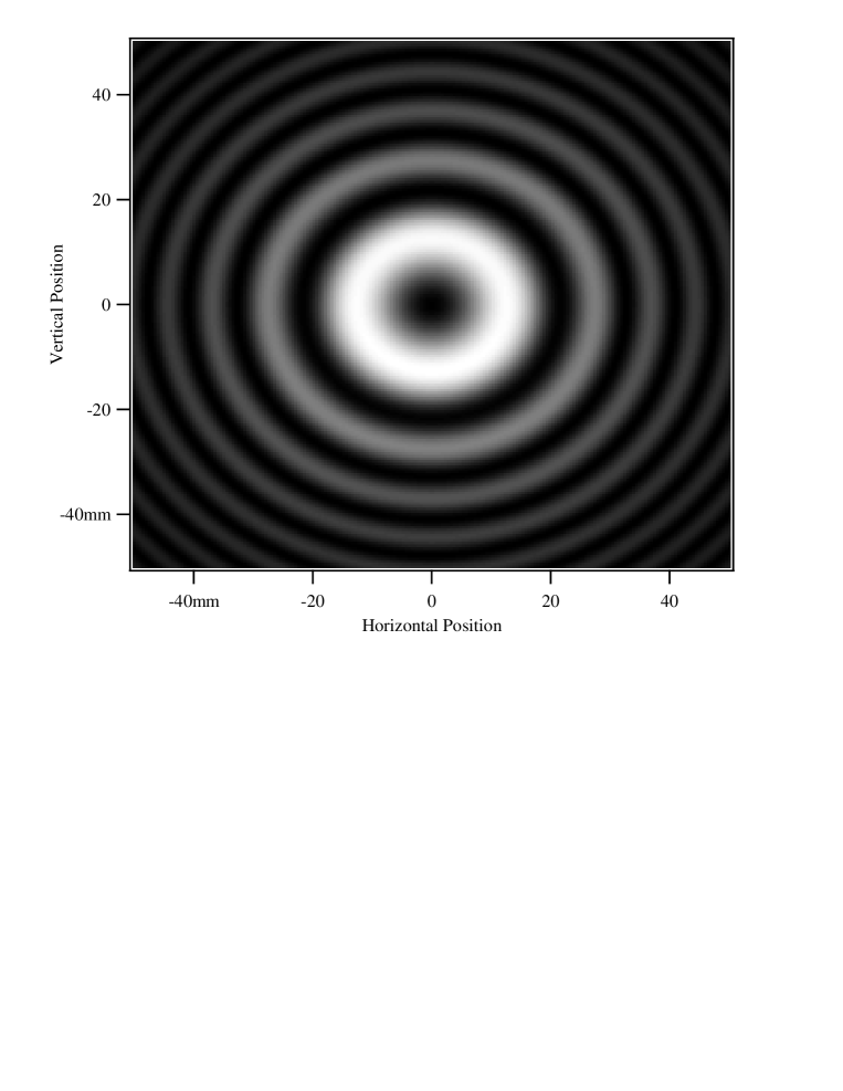
Figure 6: Contour plot of the spatial distribution of radiation simulated with the help of the SRW code at the position of the first optical element, $z=400$ m.

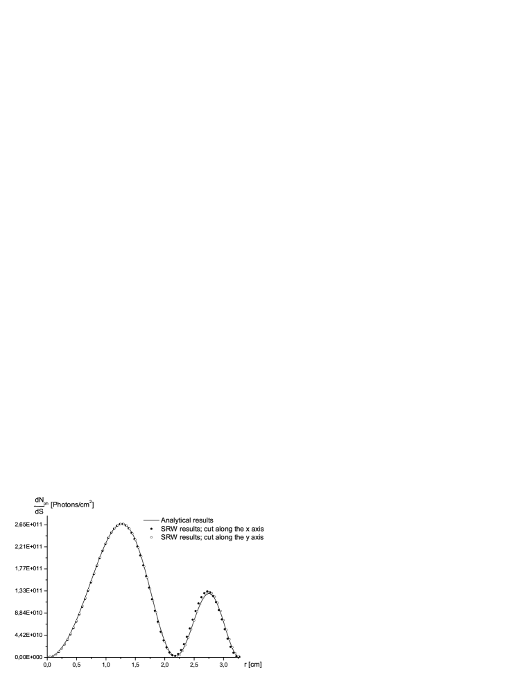
Figure 7: Photon density distribution as a function of the radial position at the first optical element, $z=400$ m. The solid line has been calculated with the help of Eq. (LABEL:fiprF). Black and white circles are obtained by cutting the contour plot in Fig. 6 respectively along the horizontal and vertical axis.

$$\vec{\widetilde{E}}\left(\pm\frac{L}{2},\vec{r}\right)=\mp\frac{2ie}{c\gamma\lambdabar}\exp\left[\pm\frac{iL}{4\gamma^{2}\lambdabar}\right]\frac{\vec{r}}{r}K_{1}\left(\frac{r}{\gamma\lambdabar}\right)~{}.$$ (13)

Fresnel propagation can now be performed, and the radiation energy density can be calculated as OURF

$$\frac{dW}{d\omega dS} = \frac{e^{2}}{4\pi^{2}\lambdabar Lc}F\left(z,\vec{r}\right)~{}$$ (14)

with

$$F\left(z,\vec{r}\right) = \left|\left\{-\frac{\vec{r}}{r}\left(\frac{2i}{{z}-L/2}\right){\frac{L}{\gamma\lambdabar\sqrt{\lambdabar L}}}\exp\left[\frac{ir^{2}}{2\lambdabar\left({z}-L/2\right)}\right]\exp\left[\frac{i}{4}\frac{L}{\gamma^{2}\lambdabar}\right]\right.\right.$$ (18)

$$\left.\left.\times\int_{0}^{\infty}d{r}^{\prime}{r}^{\prime}K_{1}\left(\frac{r^{\prime}}{\gamma\lambdabar}\right)J_{1}\left(\frac{r{r}^{\prime}}{\lambdabar({z}-L/2)}\right)\exp\left[\frac{i{r}^{\prime 2}}{2\lambdabar\left({z}-L/2\right)}\right]\right\}\right.$$

$$\left.+\left\{\frac{\vec{r}}{r}\left(\frac{2i}{{z}+L/2}\right){\frac{L}{\gamma\lambdabar\sqrt{\lambdabar L}}}\exp\left[\frac{ir^{2}}{2\lambdabar\left({z}+L/2\right)}\right]\exp\left[-\frac{i}{4}\frac{L}{\gamma^{2}\lambdabar}\right]\right.\right.$$

$$\left.\left.\times\int_{0}^{\infty}d{r}^{\prime}{r}^{\prime}K_{1}\left(\frac{r^{\prime}}{\gamma\lambdabar}\right)J_{1}\left(\frac{r{r}^{\prime}}{\lambdabar({z}+L/2)}\right)\exp\left[\frac{i{r}^{\prime 2}}{2\lambdabar\left({z}+L/2\right)}\right]\right\}\right|^{2}~{}.$$

Since we are interested in the radiation energy from a filament beam with a given longitudinal profile, we should multiply the single-electron result by the squared-modulus of the Fourier transform of the temporal profile of the bunch. Near the modulation frequency $c/\lambdabar$, a bunch with modulated Gaussian temporal profile and rms duration $\sigma_{T}$ gives

$$\bar{f}(\omega)=\frac{Na_{f}}{2}\left\{\exp\left[-\frac{\sigma_{T}^{2}}{2}\left(\omega-\frac{c}{\lambdabar}\right)^{2}\right]+\exp\left[-\frac{\sigma_{T}^{2}}{2}\left(\omega+\frac{c}{\lambdabar}\right)^{2}\right]\right\}~{},$$ (20)

where $\bar{f}(\omega)$ is the Fourier transform of the temporal profile of the bunch and $N$ is the number of electrons in the bunch.

In order to calculate the spatial density distribution of the number of photons per pulse we should integrate Eq. (14) in $d\omega$. Since we are interested in coherent emission around the modulation wavelength, we can consider the wavelength in Eq. (14) fixed. This amounts to a multiplication of Eq. (14) by

$$\int_{0}^{\infty}d\omega\left|\bar{f}(\omega)\right|^{2}=\frac{\sqrt{\pi}N^{2}a_{f}^{2}}{4\sigma_{T}}~{},$$ (21)

leading to

$$\frac{dN_{ph}}{dS}=\frac{\sqrt{\pi}}{16\pi^{2}}\frac{N^{2}\alpha a_{f}^{2}}{cL\sigma_{T}}F\left(z,\vec{r}\right)~{},$$ (22)

where $\alpha\equiv e^{2}/(\hbar c)=1/137$ is the fine structure constant.

We considered (see XFEL ) the case for $|a_{f}|=0.1$, $L=200$m, $\sigma_{T}\simeq 80$ fs and $N\simeq 6\cdot 10^{9}$ (i.e. about $1$ nC). Since the first element of the optical beamline is foreseen to be placed at about $300$ m from the separating magnet (see Fig. 2 and Fig. 8), and since we measure $z$ from the center of the straight section, we set our observation plane at $z=400$ m. Then we use Eq. (22) to calculate the photon density distribution. We cross-checked our analytical results with the code SRW CHUB . A contour plot for the photon density distribution as calculated from SRW is given in Fig. 6. Horizontal and vertical cuts along the contour plot are compared with Eq. (22) in Fig. 7. The total number of photons between the first two minima of the distribution function (at $r=0$ cm and $r\simeq 2.2$ cm respectively) is obtained integrating in $dS$. For parameters selected above, $N_{ph}\simeq 2\cdot 10^{12}$ photons.

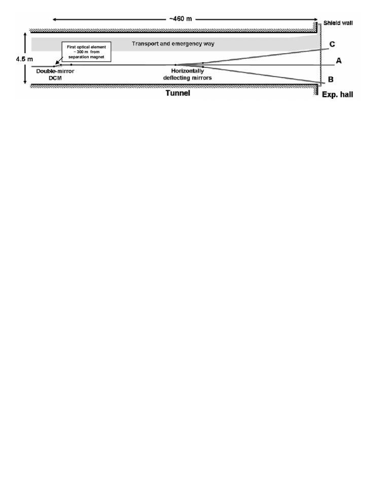
Figure 8: Schematic representation of the optical transport system in the European XFEL.

The optical pulse must be transported to the experimental area preserving relative synchronization with the XFEL pulse. The most convenient way to accomplish this task is to use the same physical support for both x-ray and edge-radiation optics, e.g. assembling mirrors for the transport of edge radiation directly on x-ray optical elements. In this way, mechanical vibrations of the transport system will not affect relative synchronization of the two pulses. A scheme of the XFEL optical system is sketched in Fig. 8. As mentioned before, the first optical elements will be located about $300$ m downstream of the separation magnet. Once edge-radiation is transported to the experimental area, single-shot cross-correlation with the pump-laser pulse can be performed, yielding the time delay between the pump-laser and the XFEL pulse. As discussed before, in reference CROS a measurement of the time-offset signal between two ultrashort laser pulses was experimentally performed based on sum-frequency generation in a non-linear crystal. The intrinsic accuracy of the method is in the femtosecond range. Actual measurements were successfully performed even when one of the two laser pulses is very weak, up to $10^{6}$ photons per pulse. This sensitivity allows our method to be employed even if a large number of optical photons are lost, from the total of $10^{12}$ photons per pulse, during the transport process along the optical system.

5 Conclusions

Our analysis demonstrates the feasibility of pump-probe experiments at XFELs with femtosecond temporal resolution, based on timing of XFEL pulses to optical pulses from an external pump-laser. The proposed scheme does not require absolute synchronization of pump and probe pulses. Synchronization in the sub-picosecond range, which has been experimentally demonstrated, is sufficient for its operation.

The present study includes an analysis of physical principles of operation, which are clear and transparent, and of fundamental physical effects of importance for the operation of the proposed time-arrival monitor.

Technical realization will be rather simple and cost-effective since it is essentially based on technical components (optical-replica synthesizer) being already included in the design of the European XFEL. Baseline parameters of the European XFEL were used in our analysis. Thus, the proposed scheme can be implemented at the first stage of XFEL facility operation.

References

- [1] A.H. Zewail, J. Phys. Chem. A, 104 (2000) 5660
- [2] M. Altarelli et al. (Eds.), XFEL: The European X-Ray Free-Electron Laser. Technical Design Report, DESY 2006-097, DESY, Hamburg (2006) (See also http://xfel.desy.de).
- [3] J. Arthur et al. Linac Coherent Light Source (LCLS). Conceptual Design Report, SLAC-R593, Stanford (2002) (See also http://www-ssrl.slac.stanford.edu/lcls/cdr).
- [4] Tanaka, T. & Shintake, T. (Eds.): SCSS X-FEL Conceptual Design Report. Riken Harima Institute, Hyogo, Japan, May 2005 (see also http://www-xfel.spring8.or.jp).
- [5] A. Winter et al., Proc. 27th Int. FEL Conference (Stanford, 2005), p.676.
- [6] J. Kim et al., Proc. 28th Int. FEL Conference (Berlin, 2006), p.287.
- [7] J. Kim et al., Proc. EPAC 2006 (Edinburgh, 2006), p.2744.
- [8] B. Faatz et al., Nucl. Instrum. and Meth. in Phys. Res. A 475 (2001), 363
- [9] J. Feldhaus et al., Nucl. Instrum. and Meth. in Phys. Res. A 528 (2004), 453
- [10] M. Gensch et al., New infrared undulator beamline at FLASH, Infrared Physics and Technology, in press.
- [11] A. A. Zholents and W. M. Fawley, Phys. Rev. Lett. 92, 224801 (2004)
- [12] E.L. Saldin, E.A. Schneidmiller and M.V. Yurkov, Proc. 29th Int. FEL Conference (Novosibirsk, 2007), TUPPH013
- [13] E. Saldin, E. Schneidmiller and M. Yurkov, Nucl. Instrum. and Meth. in Phys. Res. A 539 (2005), 499
- [14] V. Tenishev, V. Avdeichikov, A. Persson and J. Larsson, Meas. Sci. Technol. 15 (2004), 1762
- [15] P. Czonka, Part. Accel. 80 (1978) 225
- [16] E. Saldin, E. Schneidmiller and M. Yurkov, Nucl. Instrum. and Meth. in Phys. Res. A 528 (2004), 335
- [17] J. Rosenzweig et al. in Proc. of Advanced Accelerator Workshop, Lake Tahoe (1996)
- [18] G. Geloni, E. Saldin, E. Schneidmiller and M. Yurkov, Nucl. Instrum. and Meth. in Phys. Res. A 578, 1 (2007), 34
- [19] G. Geloni, E. Saldin, E. Schneidmiller and M. Yurkov, Nucl. Instrum. and Meth. in Phys. Res. A 554 (2005), 20
- [20] G. Geloni, E. Saldin, E. Schneidmiller and M. Yurkov, Nucl. Instrum. and Meth. in Phys. Res. A 583 (2007), 228
- [21] E.L. Saldin, E.A. Schneidmiller, M.V. Yurkov, Nucl. Instr. and Meth. A 429 (1999), 233
- [22] G. Geloni, E. Saldin, E. Schneidmiller and M. Yurkov, Optics Communications 276, 1 (2007), 167
- [23] R.A. Bosch et al. Rev. Sci. Instrum. 67, 3346 (1995)
- [24] R.A. Bosch and O.V. Chubar, ”Long wavelength edge radiation in an electron storage ring”, Proc. SRI’97, tenth US National Conference, AIP Conf. Proc. 417, edited by E. Fontes (AIP, Woodbury, NY), pp. 35-41 (1997)
- [25] G. Geloni, E. Saldin, E. Schneidmiller and M. Yurkov, ”Fourier Optics Treatment of Classical Relativistic Electrodynamics”, DESY 06-127 (2006) (see also http://arxiv.org/abs/physics/0608145)
- [26] K.-J. Kim, Phys. Rev. Lett. 76, 8 (1996)
- [27] B.M. Kincaid, Il Nuovo Cimento Soc. Ital. Fis, 20D, 495 (1998) and LBL-38245 (1996)
- [28] M. Castellano, Nucl. Instr and Meth. in Phys. Res. A 391 (1997) 375
- [29] R.A. Bosch, Il Nuovo Cimento, 20, 4 p. 483 (1998)
- [30] O.Chubar and P.Elleaume, in Proc. of the 6th European Particle Accelerator Conference EPAC-98, 1177-1179 (1998)