A direct Numerov sixth order numerical scheme to accurately solve the unidimensional Poisson equation with Dirichlet boundary conditions

Abstract

In this article, we present an analytical direct method, based on a Numerov three-point scheme, which is sixth order accurate and has a linear execution time on the grid dimension, to solve the discrete one-dimensional Poisson equation with Dirichlet boundary conditions. Our results should improve numerical codes used mainly in self-consistent calculations in solid state physics.

1 Introduction

The one-dimensional Poisson equation,

$$\frac{d^{2}\phi}{dx^{2}}=-\rho,\quad a\leq x\leq b,$$ (1)

with Dirichlet boundary conditions,

$$\phi(a)=c_{1},\quad\phi(b)=c_{2},$$ (2)

plays an important role in many branches of science. Particularly, the Poisson equation (1) is essential in self-consistent calculations in solid state physics [1]. In general, we have to solve it numerically many times. Therefore, is vital to have the fastest and the most accurate numerical scheme to solve it. In this article, we present a very efficient direct method, based on a Numerov [2, 3, 4] sixth order numerical scheme, to solve the Poisson equation (1) numerically. Because of its efficiency and simplicity, this new method can be used as a canonical numerical scheme to accurately solve the one-dimensional Poisson equation.

This article is organized as follows. Our numerical scheme is presented in Section 2. Its linearization, together with a few discussions, are presented in Section 3. Our conclusions are presented in Section 4.

2 The Numerov scheme

Let $\phi_{i}=\phi(x_{i})$ represents the solution of (1) at the $i$-th point, $x_{i}=a+(i-1)h$, of an equally spaced net of step $h=(b-a)/N$ and dimension $N+1$. Let also $\phi_{i}^{(k)}$ represents the $k$-th derivative evaluated at the same point $x_{i}$. Then we can evaluate the solution $\phi$ at the nearest neighborhood points $x_{i\pm 1}$ of $x_{i}$ using Taylor series [5],

$$\phi_{i\pm 1}=\phi(x_{i}\pm h)=\phi_{i}\pm\phi_{i}^{(1)}\,h+\frac{1}{2}\phi_{i}^{(2)}\,h^{2}\pm\mathcal{O}(h^{3}).$$ (3)

The basic idea in the Numerov approach is to eliminate the fourth order derivative in the expression

$$\alpha_{1}A_{1}+\alpha_{2}A_{2}=\alpha_{1}\phi_{i}-\bigl{(}\frac{h^{2}}{2}\alpha_{1}+\alpha_{2}\bigr{)}\rho_{i}+\bigl{(}\frac{h^{4}}{24}\alpha_{1}+\frac{h^{2}}{2}\alpha_{2}\bigr{)}\phi_{i}^{(4)}+\mathcal{O}(h^{6}),$$ (4)

where

$$A_{1} =\frac{1}{2}(\phi_{i+1}+\phi_{i-1})=\phi_{i}-\frac{h^{2}}{2}\rho_{i}+\frac{h^{4}}{24}\phi_{i}^{(4)}+\cdots,$$ (5)

$$A_{2} =\frac{1}{2}(\phi_{i+1}^{(2)}+\phi_{i-1}^{(2)})=-\frac{1}{2}(\rho_{i+1}+\rho_{i-1})=-\rho_{i}+\frac{h^{2}}{2}\phi_{i}^{(4)}+\cdots,$$ (6)

to obtain the sixth order three-point numerical scheme

$$\phi_{i\pm 1}=2\phi_{i}-\phi_{i\mp 1}-\frac{h^{2}}{12}\bigl{(}\rho_{i+1}+10\rho_{i}+\rho_{i-1}\bigr{)},$$ (7)

where we chose $\alpha_{1}=1$ and, consequently, $\alpha_{2}=-h^{2}/12$. In a similar way, we can eliminate the third order derivative from

$$\beta_{1}B_{1}+\beta_{2}B_{2}=h\beta_{1}\phi_{i}^{(1)}+\bigl{(}\frac{h^{3}}{6}\beta_{1}+h\beta_{2}\bigr{)}\rho_{i}^{(3)}+\mathcal{O}(h^{5}),$$ (8)

where

$$B_{1} =\frac{1}{2}(\phi_{i+1}-\phi_{i-1})=h\phi_{i}^{(1)}+\frac{h^{3}}{6}\phi_{i}^{(3)}+\cdots,$$ (9)

$$B_{2} =\frac{1}{2}(\phi_{i+1}^{(2)}-\phi_{i-1}^{(2)})=-\frac{1}{2}(\rho_{i+1}-\rho_{i-1})=-h\rho_{i}^{(3)}+\cdots,$$ (10)

to obtain the fifth order three-point numerical scheme

$$\phi_{i}^{(1)}=\frac{1}{2h}\bigl{(}\phi_{i+1}-\phi_{i-1}\bigr{)}+\frac{h^{2}}{6}\bigl{(}\rho_{i+1}-\rho_{i-1}\bigr{)},$$ (11)

for the first derivative of $\phi$, where we chose $\beta_{1}=1$ and, consequently, $\beta_{2}=-h^{2}/6$.

So far, the three-point numerical scheme (11) is an iterative method, i.e., given two informations, $\phi_{i-1}$ and $\phi_{i}$, we can calculate $\phi_{i+1}$. One difficulty of this iterative method is related with the Dirichlet boundary conditions (2): they are known only at end-points $x_{1}$ and $x_{N+1}$. Thus, we can not initiate our iterative scheme (11). Fortunately, the recurrence relation in (11) is linear with constant coefficients. These two features imply we can find an unique solution to it,

$$\phi_{i}=(i-1)\phi_{2}-(i-2)\phi_{1}-\frac{h^{2}}{12}\sum_{j=3}^{i}(i+1-j)(\rho_{j}+10\rho_{j-1}+\rho_{j-2}),$$ (12)

where $\phi_{1}=c_{1}$ and $\phi_{2}$ must be expressed in terms of $\phi_{N+1}=c_{2}$ (the Dirichlet boundary conditions),

$$\phi_{2}=\frac{1}{N}\phi_{N+1}+(1-\frac{1}{N})\phi_{1}+\frac{h^{2}}{12N}\sum_{j=3}^{N+1}(N+2-j)(\rho_{j}+10\rho_{j-1}+\rho_{j-2}).$$ (13)

Now we have an analytical sixth order numerical scheme to solve accurately the Poisson equation (1) with the Dirichlet boundary conditions (2).

It should be mentioned that the analytical third order numerical scheme presented by Hu and O’Connell [6], making use of tridiagonal matrices, can also be derived by the present approach restricted to the third order,

$$\phi_{i}=(i-1)\phi_{2}-(i-2)\phi_{1}-h^{2}\sum_{j=3}^{i}(i+1-j)\rho_{j-1},$$ (14)

where

$$\phi_{2}=\frac{1}{N}\phi_{N+1}+(1-\frac{1}{N})\phi_{1}+h^{2}\sum_{j=3}^{N+1}(N+2-j)\rho_{j-1}.$$ (15)

3 Discussions

Although we have found a very accurate analytical direct method to solve the one-dimensional Poisson equation with Dirichlet boundary conditions, namely, the sixth order Numerov scheme (11), it has one undesirable feature: its execution time is proportional to the square of the grid dimension. Fortunately it can be linearized. First, we create a vector $U$, whose components are the partial sums $U_{i}=\rho_{i}+10\rho_{i-1}+\rho_{i-2}$ ($U_{1}=U_{2}=0$). Next, we create a second vector $V$ with $V_{i}=V_{i-1}+U_{i}$ and $V_{1}=V_{2}=0$. We also need a third vector $Y$ with $Y_{i}=iU_{i}$ and a fourth vector $Z$ with the complete sums $Z_{i}=Z_{i-1}+Y_{i}$. Using these new vectors, our sixth order Numerov scheme (11) can be rewritten as follows,

$$\phi_{i}=(i-1)\phi_{2}-(i-2)\phi_{1}-\frac{h^{2}}{12}\bigl{[}(i+1)V_{i}-Z_{i}\bigr{]}.$$ (16)

This numerical scheme has now a linear execution time proportional to five times the grid dimension $N+1$.

Let us use a Gaussian density,

$$\rho(x)=\mathrm{e}^{-x^{2}/4},$$ (17)

to verify the accuracy and the efficiency of the non-linear numerical scheme (12), as well as the linear numerical scheme (16). The solution for the Poisson equation (1), along with the boundary conditions $\phi(-10)=\phi_{1}=1$ and $\phi(+10)=\phi_{N+1}=2$, is

$$\phi(x)=\frac{x}{20}-\sqrt{\pi}\,x\,\mathrm{erf}(x/2)-2\mathrm{e}^{-x^{2}/4}+\frac{3}{2}+10\sqrt{\pi}\,\mathrm{erf}(5)+2\mathrm{e}^{-25},$$ (18)

where $\mathrm{erf}(x)$ is the error function,

$$\mathrm{erf}(x)=\frac{2}{\sqrt{\pi}}\int_{0}^{x}\mathrm{e}^{-t^{2}}\,dt.$$ (19)

Figure 1(a) shows the execution time as a function of the grid dimension $N+1$ for three cases. In one case (the dotted line), the numerical solution was computed by the non-linear third order numerical scheme (14). In the second case (the dashed line), the numerical solution was computed by the non-linear sixth order numerical scheme (12). In the last case (the solid line), the numerical solution was computed by the linear sixth order numerical scheme (16). At $N=1000$, the execution time of the non-linear third (sixth) order numerical scheme is approximately 145 (51) times the execution time of the linear sixth order numerical scheme. Clearly, we can see that the linearization process described above plays an essential role in the present Numerov scheme.

In order to measure the accuracy of the present Numerov scheme, we can compute the Euclidean norm

$$||W_{N}||=\sqrt{\sum_{i=1}^{N+1}\biggl{[}\Phi^{(e)}(x_{i})-\Phi^{(n)}_{i}\biggr{]}^{2}}$$ (20)

where $\Phi^{(e)}$ stands for the exact solution (18) and $\Phi^{(n)}$ stands for the numerical solution. Figure 1(b) shows (right vertical axis) a comparasion between two Euclidean norms (20): one (dashed line) using the third-order numerical scheme (14) and the other (solid line) using the sixth-order numerical scheme (16). Note that, at $N=400$, the exact Euclidean norm of the third-order scheme is approximately four orders of magnitude above the exact Euclidean norm of the sixth-order scheme. Naturally, we can see that the sixth-order numerical scheme (16) is much more accurate and efficient than the third-order numerical scheme (12). Of course, we don’t know the exact solution in practical applications. In that case, the best we can do is to compute the mean Euclidean norm of the numerical solution $\Phi^{(n)}$,

$$||\Phi_{N}||=\sqrt{\frac{1}{N}\sum_{i=1}^{N+1}\biggl{(}\Phi_{i}^{(n)}\biggr{)}^{2}}.$$ (21)

This mean Euclidean norm can be used as a convergency criterion, as shown in Figure 1(b) (left vertical axis).

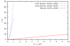
(a) Execution times

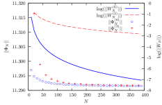
(b) Euclidean norms

Figure 1: Execution times (a) and exact ($||W_{N}||$) and mean ($||\Phi_{N}||$) Euclidean norms (b) as functions of the grid dimension $N+1$. The exact solution is given in (18) and corresponds to the Gaussian density (17) with boundary conditions $\phi_{1}=1$ and $\phi_{N+1}=2$

4 Conclusions

We have applied the Numerov method to derive a sixth-order numerical scheme to solve the one-dimensional Poisson equation (1) with Dirichlet boundary conditions. The resulting recurrence relations were exactly solved and the corresponding execution time was linearized [see (16)] in such way to avoid the handling of a dense matrix. Therefore, the numerical scheme (16) is both accurate and efficient as illustrated in Figure 1. Moreover, it is extremely ease to implement in any numerical or algebraic computer language. As pointed by J. M. Blatt [3], the Numerov method is both a three-point method, which implies it is stable, and of highest order, which implies it is accurate. All these features make the numerical scheme (16) the canonical method of choice for the integration of the Poisson equation (1).

References

[1]
E. A. Johnson.
Low-dimensional Semiconductor Structures.
Cambridge, 2001.
[2]
B. V. Numerov.
A method of extrapolation of perturbations.
Roy. Ast. Soc. Monthly Notices, 84:592, 1924.
[3]
J. M. Blatt.
Pratical points concerning the solution of the Schrödinger
equation.
J. Comp. Phys., 1:382, 1967.
[4]
R. P. Agarwal and Y. M. Wang.
Some recent developments of Numerov’s method.
Comp. Math. App., 0:561, 2001.
[5]
J. W. Thomas.
Numerical Partial Differential Equations. Finite Difference
Methods., volume 22 of Texts in Applied Mathematics.
Springer, 1995.
[6]
G. Y. Hu and R. F. O’Connell.
Analytical inversion of symmetric tridiagonal matrices.
J. Phys. A: Math. Gen., 29:1511, 1996.