Approximating Data with weighted smoothing Splines

Abstract

Given a data set $(t_{i},y_{i})$, $i=1,\dots,n$ with the $t_{i}\in[0,\,1]$ non-parametric regression is concerned with the problem of specifying a suitable function $f_{n}:[0,\,1]\rightarrow\mathbb{R}$ such that the data can be reasonably approximated by the points $(t_{i},f_{n}(t_{i}))$, $i=1,\dots,n.$ If a data set exhibits large variations in local behaviour, for example large peaks as in spectroscopy data, then the method must be able to adapt to the local changes in smoothness. Whilst many methods are able to accomplish this they are less successful at adapting derivatives. In this paper we show how the goal of local adaptivity of the function and its first and second derivatives can be attained in a simple manner using weighted smoothing splines. A residual based concept of approximation is used which forces local adaptivity of the regression function together with a global regularization which makes the function as smooth as possible subject to the approximation constraints.
AMS 2000 Subject classifications: Primary 62G08, secondary 62G15, 62G20
Keywords: nonparametric regression, smoothing splines, confidence region, regularization

1 Introduction

1.1 Smoothing and weighted smoothing splines

In the one-dimensional case nonparametric regression is concerned with determining a function $f_{n}:[0,\,1]\rightarrow\mathbb{R}$ which adequately represents a data set ${\mbox{\boldmath$y$}}_{n}=\{(t_{i},y(t_{i})):t_{i}\in[0,\,1],\,i=1,\ldots,n\}.$ The problem is to provide a function $f_{n}$ which is an adequate representation of the data. One well established method for accomplishing this goal is that of smoothing splines defined as the solution of the problem

$$\min S(g,\lambda):=\sum_{i=1}^{n}(y(t_{i})-g(t_{i}))^{2}+\lambda\int_{0}^{1}g^{(2)}(t)^{2}\,dt$$ (1)

where $\lambda$ is the smoothing parameter (see Wahba, (1990); Green and Silverman, (1994); Ruppert et al., (2003)). This approach has two weaknesses. The first is that there may not be any choice of $\lambda$ for which the resulting fit is satisfactory. This is particularly the case if the data show large local variations such as in Figure 1 which are taken from thin film physics. They were kindly supplied by Prof. Dieter Mergel of the Department of Physics, University of Duisburg-Essen. X-rays are beamed onto a thin film and the data give the photon count of the diffracted rays as a function of the angle of diffraction. The sample size is $n=7001.$ The high peaks can only be adequately captured with a small value of $\lambda$ in (1). This has however the consequence that the function oscillates too rapidly between the peaks. The second problem is to give an automatic choice for $\lambda.$ Methods suggested include cross-validation, generalized cross-validation, generalized maximum likelihood and restricted maximum likelihood (Craven and Wahba, (1978); Wahba, (1985); Ruppert et al., (2003)). However it is clear that if there is no satisfactory value of $\lambda$ then no automatic choice will work.

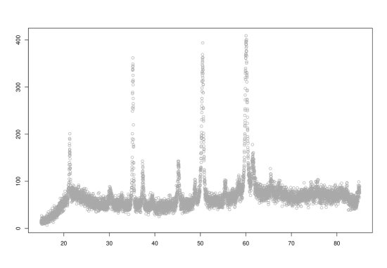
Figure 1: Data from thin-film physics showing the photon count of X-rays as a function of the angle of diffraction measured in degrees.

In this paper we attain more flexibility by considering a vector ${\mbox{\boldmath$\lambda$}}=(\lambda_{1},\ldots,\lambda_{n})$ rather than a single value $\lambda$ and we replace the minimization problem (1) by

$$\min S(g,{\mbox{\boldmath$\lambda$}}):=\sum_{i=1}^{n}\lambda_{i}(y(t_{i})-g(t_{i}))^{2}+\int_{0}^{1}g^{(2)}(t)^{2}\,dt.$$ (2)

Comparing this with (1) we see that the smoothing parameter $\lambda$ has now been transferred from the penalty term to the observations themselves. The solution, which we denote by $f_{n}(\cdot:{\mbox{\boldmath$\lambda$}}),$ is a natural cubic spline (see Green and Silverman, (1994)) but the $\lambda_{i}$ now control the fit at the observation points $(t_{i},y(t_{i}))$ rather than the size of the penalty which is now fixed. In the case of the data displayed in Figure 1 we would choose large values of $\lambda_{i}$ at the peaks causing them to be adequately approximated. At points away from the peaks we would choose the $\lambda_{i}$ to be small and thus ensure a smooth solution at these points.

The method proposed here belongs to the category of spatially adaptive splines. For other spatially adaptive spline methods we refer to Luo and Wahba, (1997), Denison et al., (1998), Ruppert and Carroll, (2000), Zhou and Shen, (2001), DiMatteo et al., (2001), Pittman, (2002), Wood et al., (2002), Miyata and Shen, (2003, 2005), Pintore et al., (2006).

1.2 Contents

In Section 2 we describe an approach to choosing a model in the context of nonparametric regression which is based on a universal, honest and non-asymptotic confidence region. Section 3 shows how the ideas of Section 2 can be adapted to give a simple method for choosing the weights of a weighted smoothing spline. Examples and the results of a small simulation study are given in Section 4. Section 5 gives two variations on this theme and Section 6 extends the method to image analysis. Finally in Section 7 we look at the asymptotics.

2 Choosing a model

2.1 Nonparametric confidence regions

A lot of work has been devoted to choosing a model from a sequence of models of increasing complexity. Choosing a value of $\lambda$ in (1) falls into this category as the smaller $\lambda$ the more complex the resulting smoothing spline. Methods developed to solve the problem include cross-validation, plug-in methods as well as AIC and BIC which are explicitly phrased in terms of balancing complexity and fidelity. We take a different approach here which is implicit in Davies and Kovac, (2004) and explicit in Davies et al., 2008b . We define a universal, honest and non-asymptotic confidence region ${\mathcal{A}}_{n}$ and given this region we choose non-decreasing $\lambda_{i}^{j},\,j=1,2,\ldots$ to force $f_{n}(\cdot:{\mbox{\boldmath$\lambda$}}^{j})$ to eventually lie in ${\mathcal{A}}_{n}.$ This gives a sequence of functions of increasing roughness (or complexity) and we choose the first one which lies in ${\mathcal{A}}_{n}.$ The region ${\mathcal{A}}_{n}$ is based on the residuals and requires a stochastic model. The one we use is

$$Y(t)=f(t)+\sigma Z(t),\quad 0\leq t\leq 1$$ (3)

with $Z(t)$ standard Gaussian white noise. Following Davies et al., 2008b ${\mathcal{A}}_{n}$ is defined as follows. For any function $g$ we consider normalized sums of residuals over intervals

$$w({\mbox{\boldmath$y$}}_{n},I,g)=\frac{1}{\sqrt{|I|}}\,\sum_{t_{i}\in I}(y(t_{i})-g(t_{i}))$$ (4)

where $|I|$ denotes the number of points $t_{i}$ in the interval $I.$ For data ${\mbox{\boldmath$Y$}}_{n}={\mbox{\boldmath$Y$}}_{n}(f)$ generated under the model (3) we define the confidence region for $f$ by

$${\mathcal{A}}_{n}={\mathcal{A}}_{n}({\mbox{\boldmath$Y$}}_{n},\sigma,{\mathcal{I}}_{n},\tau_{n})=\big{\{}g:\max_{I\in{\mathcal{I}}_{n}}\,|w({\mbox{\boldmath$Y$}}_{n},I,g)|\leq\sigma\sqrt{\tau_{n}\log n\,}\,\big{\}}$$

where ${\mathcal{I}}_{n}$ is a family of intervals and $\tau_{n}=\tau_{n}(\alpha)$ is defined by

$$P\Big{(}\max_{I\in{\mathcal{I}}_{n}}\frac{1}{\sqrt{|I|}}\Big{|}\sum_{i\in I}Z(t_{i})\Big{|}\leq\sqrt{\tau_{n}\log n\,}\,\Big{)}=\alpha.$$ (5)

It follows that ${\mathcal{A}}_{n}({\mbox{\boldmath$Y$}}_{n},\sigma,{\mathcal{I}}_{n},\tau_{n})$ is a universal, honest and non-asymptotic confidence region for $f$, that is

$${\mbox{\boldmath$P$}}(f\in{\mathcal{A}}_{n}({\mbox{\boldmath$Y$}}_{n}(f),\sigma,{\mathcal{I}}_{n},\tau_{n}))=\alpha\quad\text{for all}\,\,f\,\,\text{and}\,\,n.$$

The family of intervals ${\mathcal{I}}_{n}$ can be taken to be the family of all intervals but this is computationally expensive. For all practical purposes it suffices to consider a subfamily of intervals as long as it is multiscale, that is, if it contains intervals of all sizes. The simplest such scheme, and the one we shall use, corresponds closely to that defined by the Haar wavelet. If $n=2^{m}$ the family ${\mathcal{I}}_{n}$ consists of all one-point intervals $[t_{1},t_{1}]\ldots,[t_{n},t_{n}]$, all two point intervals $[t_{1},t_{2}],[t_{3},t_{4}],\ldots,[t_{n-1},t_{n}]$, all four-point intervals $[t_{1},t_{4}],[t_{5},t_{8}],\ldots,[t_{n-3},t_{n}]$ and so forth. If $n$ is not a power of 2 we simply include the last interval whatever its form. In the remainder of the paper we use this dyadic scheme. For any scheme ${\mathcal{I}}_{n}$ and for given $\alpha$ the values of $\tau_{n}(\alpha)$ as defined by (5) can be obtained by simulations. Table 1 gives the values of $\tau_{n}(\alpha)$ for the dyadic scheme just described, $\alpha=0.95$ and 0.99 and for various sample sizes $n.$ The results are based on 10000 simulations.

$n$	100	250	500	1000	2500	5000	10000
0.95	2.92	2.88	2.79	2.71	2.64	2.60	2.55
0.99	3.60	3.41	3.33	3.17	3.03	3.00	2.92

Table 1: The values of $\tau_{n}(\alpha)$ for the dyadic scheme ${\mathcal{I}}_{n},\,\alpha=0.95$ and 0.99 and $n=100,\,250,\,500,\,1000,\,2500,\,5000$ and 10000.

It follows from a result of Dümbgen and Spokoiny, (2001) and the very precise result of Kabluchko, (2007) that if ${\mathcal{I}}_{n}$ contains all one-point intervals then

$$\lim_{n\rightarrow\infty}\tau_{n}(\alpha)=2$$

for all $\alpha.$ In particular this holds for the dyadic multiscale family ${\mathcal{I}}_{n}$ we consider. The resulting curves are not sensitive to the value of $\tau_{n}(\alpha)$ and so for simplicity in the remainder of the paper we simply put $\tau_{n}(\alpha)=3.$ This is consistent with the values of Table 1.

An Associate Editor asked to what extent the results depend on the chosen scheme ${\mathcal{I}}_{n}$ and the value of $\tau_{n}.$ This can be analysed as follows. Suppose the data are generated by a function $f$ and consider a function ${\tilde{f}}_{n}$ which differs from $f$ by $\delta_{n}$ on an interval $I$, that is ${\tilde{f}}_{n}(t)-f(t)>\delta_{n},\,t\in I.$ This will be detected by the procedure if ${\tilde{f}}_{n}\notin{\mathcal{A}}_{n}.$ If ${\mathcal{I}}_{n}$ is the family of all intervals then ${\tilde{f}}_{n}\notin{\mathcal{A}}_{n}$ follows from

$$\frac{1}{\sqrt{|I|}}\sum_{t_{i}\in I}(Y(t_{j})-{\tilde{f}}(t_{j}))\leq-\sigma\sqrt{\tau_{n}\log n}.$$

From this we deduce that the deviation will be detected with probability at least $\alpha-0.01$ if

$$\delta_{n}\geq\sigma\Big{(}\sqrt{\tau_{n}\log n}+2.3263\Big{)}/\sqrt{|I|}\,.$$ (6)

If we use the dyadic scheme ${\mathcal{I}}_{n}^{\prime}$ it is no longer guaranteed that $I\in{\mathcal{I}}_{n}^{\prime}.$ However there exists an interval $I^{\prime}\subset I$ in ${\mathcal{I}}_{n}^{\prime}$ with $|I^{\prime}|\geq|I|/2.$ The same argument gives

$$\delta_{n}\geq\sigma\sqrt{2}\Big{(}\sqrt{\tau_{n}^{\prime}\log n}+2.3263\Big{)}/\sqrt{|I|}\,$$ (7)

Denser schemes ${\mathcal{I}}_{n}(\kappa)$ parameterized by a parameter $\kappa,\,1<\kappa\leq 2,$ with $|{\mathcal{I}}_{n}(\kappa)|=O(n)$ are given in Davies et al., 2008b : the dyadic scheme corresponds to the case $\kappa=2$. If we use ${\mathcal{I}}_{n}(\kappa)$ then we can replace (7) by

$$\delta_{n}\geq\sigma\sqrt{\kappa}\Big{(}\sqrt{\tau_{n}(\kappa)\log n}+2.3263\Big{)}/\sqrt{|I|}\,.$$

As $\tau_{n}(\kappa)<\tau_{n}$ this can be made arbitrarily close to the case of all intervals (6). The dyadic scheme is the coarsest we use, but it is nevertheless efficacious as shown by the results of Davies et al., 2008a . The analysis we have done is for a worst-case situation, the actual performance may be better. As an example we take $\alpha=0.95,\,\sigma=1$ and $n=1000.$ It follows from Table 1 that the value of $\tau_{n}^{\prime}$ in (7) is 2.71. Simulations show that the corresponding value of $\tau_{n}$ in (6) is 2.91. If $|I|=24$ then we have $\delta_{n}\geq 1.39$ for (6) and $\delta_{n}\geq 1.92$ for (7). The upper panel of Figure 2 shows standard white noise $f\equiv 0$: the lower panel shows ${\tilde{f}}_{n}(t)+Z(t)$ for the same noise with ${\tilde{f}}(t)=\delta$ for $0.5<t\leq 0.524,$ zero otherwise and $\delta=0.7.$

Figure 2: The upper panel shows standard white noise $Z(t)$. The lower panel shows $f^{\prime}(t)+Z(t)$ with ${\tilde{f}}_{n}(t)=0.7$ for $0.5<t\leq 0.524$ and zero otherwise.

The signal in the lower panel is difficult to detect by eye: the signal-to-noise ratio is 0.11. However it is detected using the dyadic scheme with $\tau_{n}=3$. If we put $\tau_{n}=2.71$ then a signal with $\delta=0.63$ is detected. If we use all intervals then with $\tau_{n}=3$ a signal with $\delta=0.67$ is detected, for $\tau_{n}=2.91$ a signal with $\delta=0.64$ is detected. The differences are not large.

So far we have assumed that $\sigma$ is known which is not the case. We use the default value (Davies and Kovac, (2001))

$$\sigma_{n}=\frac{1.4826}{\sqrt{2}}\text{MED}\{|y(t_{i})-y(t_{i-1})|,i=2,\dots,n-1\}.$$ (8)

For data generated under the model we have

$$Y(t_{i})-Y(t_{i-1})=Z(t_{i})-Z(t_{i-1})+f(t_{i})-f(t_{i-1}).$$

If $Z$ is a $N(0,1)$ random variable it may be checked that the median of $|Z-c|$ strictly exceeds that of $|Z|$ for any $c\neq 0.$ From this it follows that $\sigma_{n}$ is always biased upwards under the model. Consequently ${\mathcal{A}}_{n}({\mbox{\boldmath$Y$}}_{n},\sigma_{n},{\mathcal{I}}_{n},\tau_{n})$ is no longer a universal, exact, non-asymptotic confidence region but it is a universal, honest (Li, (1989)), non-asymptotic confidence region

$${\mbox{\boldmath$P$}}(f\in{\mathcal{A}}_{n}({\mbox{\boldmath$Y$}}_{n},\sigma_{n},{\mathcal{I}}_{n},\tau_{n}))\geq\alpha\quad\text{for all}\,\,f\,\,\text{and}\,\,n.$$

Given the confidence region ${\mathcal{A}}_{n}({\mbox{\boldmath$y$}}_{n},\sigma_{n},{\mathcal{I}}_{n},\tau_{n})$ and the measure of roughness

$$R(g)=\int_{0}^{1}g^{(2)}(t)^{2}\,dt$$

the natural approach would be to solve

$$\text{minimize}\quad R(g)\quad\text{subject to}\quad g\in{\mathcal{A}}_{n}({\mbox{\boldmath$y$}}_{n},\sigma_{n},{\mathcal{I}}_{n},\tau_{n}).$$ (9)

As ${\mathcal{A}}_{n}$ is defined by a set of linear inequalities involving the values of $g$ at the points $t_{i}$ the problem is one of quadratic programming. If we take the dyadic scheme for ${\mathcal{I}}_{n}$ then ${\mathcal{A}}_{n}$ is defined by about $4n$ linear inequalities. For small data sets with $n\leq 1000$ which exhibit little local variability it is possible to solve this directly but the approach fails for data sets such as those of Figure 1 with $n=7001.$ The quadratic programming problem involves 7001 parameters and the number of linear constraints is about 28000. Furthermore the fact that the squared second derivative varies by several orders of magnitude over the interval causes excessive numerical instability. In contrast the problem (2) can be solved for in a fast and stable manner even for values of $\lambda_{i}$ which differ by orders of magnitude. In the next section we describe an automatic procedure for doing this which attempts to emulate the solution of (9).

The idea of the confidence region as defined above is implicit in Davies and Kovac, (2001). A similar idea was used by Dümbgen and Spokoiny (2001) for testing for monotonicity and convexity of nonparametric functions. Universal, exact, non-asymptotic confidence regions based on the signs of the residuals $\text{sign}(y(t_{i})-g(t_{i}))$ rather than the residuals themselves are to be found implicitly in Davies, (1995) and explicitly in Dümbgen, (2003, 2007) and Dümbgen and Johns, (2004). These require only that under the model the errors are independently distributed with median zero. As a consequence they do not require an auxiliary estimate of scale such as (8).

3 Choosing the weights

3.1 The procedure

The procedure we use is based on the following heuristic. If $\|{\mbox{\boldmath$\lambda$}}\|$ is small then the solution $f_{n}(\cdot:{\mbox{\boldmath$\lambda$}})$ of (2) will be essentially the least squares line through the data. If on the other hand all the components $\lambda_{i}$ of $\lambda$ are very large then $f_{n}(\cdot:{\mbox{\boldmath$\lambda$}})$ will almost interpolate that data and will lie in ${\mathcal{A}}_{n}$ as all residuals will be close to zero. The idea is then to start with very small $\lambda_{i}$ and then to increase them gradually until $f_{n}(\cdot:{\mbox{\boldmath$\lambda$}})$ lies in ${\mathcal{A}}_{n}$ and then stop. More formally we start with the least squares regression line and check whether this lies in ${\mathcal{A}}_{n}$. If so we stop and accept the solution. Otherwise put ${\mbox{\boldmath$\lambda$}}^{1}=(\lambda_{1},\ldots,\lambda_{1})$ where $\lambda_{1}$ is chosen to be so small that the solution of (2) with ${\mbox{\boldmath$\lambda$}}={\mbox{\boldmath$\lambda$}}^{1}$ differs from the least squares lines by some small prescribed quantity. At the $i$th stage we have the solution $f_{n}(\cdot:{\mbox{\boldmath$\lambda$}}^{i})$ based on the weights ${\mbox{\boldmath$\lambda$}}^{i}.$ We check if the solution lies in ${\mathcal{A}}_{n}$ and if so we stop. If not we determine those intervals $I_{i}\in{\mathcal{I}}_{n}$ for which

$$w({\mbox{\boldmath$y$}}_{n},I_{i},f_{n}(\cdot:{\mbox{\boldmath$\lambda$}}^{i}))\geq\sigma_{n}\sqrt{\tau_{n}\log n}.$$ (10)

For all points $t_{j}$ in any such interval we increase the corresponding $\lambda_{j}^{i}$ by a factor of $q$, that is $\lambda_{j}^{i+1}=q\lambda_{j}^{i}.$ Our default value for $q$ is 2. The remaining $\lambda_{j}^{i}$ are not altered. This gives us a new ${\mbox{\boldmath$\lambda$}}^{i+1}$ and we repeat the procedure.

As defined the procedure is difficult to analyse, especially as the effect is a finite sample one: it will gradually disappear for a fixed function $f$ as the sample size $n$ tends to infinity. The problem can be circumnavigated to a certain extent as follows. We consider a second procedure but this time with the components $\lambda^{i}_{j}$ of ${\mbox{\boldmath$\lambda$}}^{i}$ all equal, $\lambda^{i}_{j}=\lambda^{i},j=1,\ldots,n.$ If the solution does not lie in ${\mathcal{A}}_{n}$ then all components are increased by a factor of $q$ and not just those whose $t_{j}$ values lie in intervals $I_{i}$ for which (10) holds. For this form of ${\mbox{\boldmath$\lambda$}}=(\lambda,\ldots,\lambda)$ it can be shown that $R(f_{n}(\cdot:{\mbox{\boldmath$\lambda$}}))$ depends monotonically on $\lambda$ which makes it amenable to mathematical analysis. If we now perform both procedures and then choose at the end the smoothest of the two solutions we have a procedure which can be analysed. We have not yet encountered a data set where the result of the second procedure with equal weights was chosen. We point out that solving (2) for this form of ${\lambda}$ is equivalent to solving (1) but with $\lambda^{-1}$ in place of $\lambda.$ The second procedure therefore does the following. It considers the one-dimensional family of solutions of (1) and chooses the smoothest such function which lies in ${\mathcal{A}}_{n}.$ This is an alternative to choosing the smoothing parameter by cross-validation or likelihood methods.

3.2 An illustration

We apply the procedure to the thin film data of Figure 1. The value of $\sigma_{n}$ of (8) is 8.3868. With $n=7001$ and $\tau_{n}(\alpha)=3$ we have

$$\sigma_{n}\sqrt{\tau_{n}(\alpha)\log n}=8.3868\sqrt{3\cdot\log 7001}=43.22$$

The upper panel of Figure 3 shows the resulting curve: the lower panel shows the associated values of the $\lambda_{i}$ on a logarithmic scale. It is noticeable that the values of the $\lambda_{i}$ are large in the neighbourhoods of the large peaks and small outside of these. The manner in which the curve alters in the course of the iterations is shown on a larger scale in Figure 4. The rows show the results after 1, 15 and 25 iterations and the final result after 33 iterations for the first 1000 observations. In each case the left panel shows the curve and the right panel the weights $\lambda_{i}$ on a logarithmic scale. Initially the weights are constant with a value of $2.9\cdot 10^{-8}.$ After 15 iterations they are still constant but now with the common value $2.5\cdot 10^{-4}.$ After 25 iterations the smallest weights are $7.4\cdot 10^{-3}$ and the largest is 0.18. The smallest weights for the final curve are still $7.4\cdot 10^{-3}$ but the largest weight is now 20. The values of the $\lambda_{i}$ differ by a factor of 30000. The final row shows the advantage of the local weights $\lambda_{i}.$ Where the data can be fitted with a smooth curve the $\lambda_{i}$ are small and the fit is smooth. Where there is a pronounced peak the values of the $\lambda_{i}$ are large and this forces the solution of (1) to adjust to the peak.

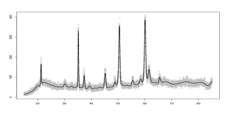
Figure 3: The upper panel shows the results of applying the weighted smoothing spline procedure to the thin film data. The lower panel shows the values of the $\lambda_{i}$ on a logarithmic scale.

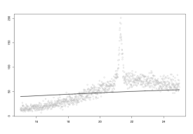
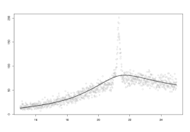
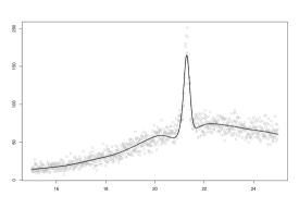
Figure 4: The rows show the results after 1, 15, 25 and 33 iterations of the weighted smoothing splines procedure to the first 1000 data points of the thin film data. The left panel shows the curve and the right panel the weights $\lambda_{i}$ on a logarithmic scale.

4 Examples and simulations

4.1 The thin film data

The estimators we consider are the weighted smoothing spline (wss), the spatially adaptive spline method due to Ruppert and Carroll, (2000) and the standard smoothing spline (smspl) with smoothing parameter chosen by cross validation. The Ruppert–Carroll method uses so called ‘penalized splines’ which are the p-splines of Eilers and Marx, (1996) (see also O’Sullivan, (1986, 1988)). In contrast to smoothing splines they use a spatially weighted penalty term with the weights being determined by generalized cross-validation. The method is not fully automatic and requires the specification of the maximum number of knots. Based on Ruppert and Carroll, (2000) the numbers we choose are 40, 80, 160 and 320: we denote the corresponding estimators by pspl40, pspl80, pspl160 and pspl320. Figure 5 shows the results for the complete data set. It is seen that the peaks are satisfactorily captured only by the wss, pspl320 and smspl reconstructions. Figure 6 shows the results for the first 1000 observations only for these three methods. Only the wss succeeds in capturing the peaks and giving a smooth reconstruction between the peaks.

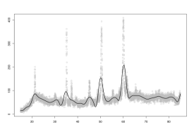
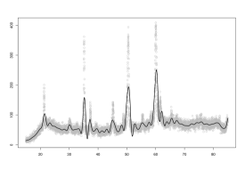
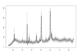
Figure 5: The top row shows from left to right the wss and pspl40 reconstructions, the centre row the results for the pspl80 and pspl160 reconstructions and the bottom row the results for the pspl320 and the smspl reconstructions.

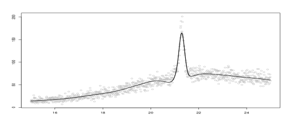
Figure 6: The first 1000 observation of the thin film data with the (from top to bottom) wss, pspl320 and smspl reconstructions.

4.2 Some simulation results

We give the results of a small simulation study using the functions of Ruppert and Carroll, (2000)

$$f(x)=f(x;j)=\sqrt{x(1-x)}\sin\left(\frac{2\pi(1+2^{(9-4j)/5)}}{x+2^{(9-4j)/5}}\right)$$

with $j=6$ and the bumps data of Donoho and Johnstone, (1995). We consider signal to noise ratios of 3 and 7. The tables gives the median (MRISE) of the root integrated square error

$$\text{RISE}(f,{\hat{f}}_{n})=\left(\int_{0}^{1}(f(t)-{\hat{f}}_{n}(t))^{2}\,dt\right)^{1/2}$$

for the fit itself and the first and second derivatives $\text{MRISE}(f^{(i)},{\hat{f}}_{n}^{(i)}),i=1,2.$ The results are based on 1000 simulations.

$\sigma=0.288/7\approx 0.0411$
	Fit				First derivative				Second derivative
	400	800	1600	3200	400	800	1600	3200	400	800	1600	3200
wss	0.030	0.021	0.016	0.012	0.267	0.161	0.096	0.057	3.98	1.88	0.85	0.37
pspl40	0.062	0.058	0.057	0.056	0.559	0.388	0.274	0.192	6.48	3.33	1.69	0.85
pspl80	0.027	0.021	0.017	0.015	0.339	0.218	0.145	0.101	5.26	2.69	1.32	0.67
pspl160	0.022	0.016	0.012	0.009	0.244	0.148	0.090	0.054	3.87	2.12	1.14	0.56
smspl	0.024	0.016	0.012	0.009	0.294	0.139	0.080	0.047	4.77	1.77	0.79	0.37
$\sigma=0.288/3\approx 0.096$
	Fit				First derivative				Second derivative
	400	800	1600	3200	400	800	1600	3200	400	800	1600	3200
wss	5.60	2.71	1.22	0.54	0.417	0.244	0.150	0.093	5.60	2.71	1.22	0.54
pspl40	6.49	3.34	1.69	0.85	0.567	0.392	0.275	0.193	6.49	3.34	1.69	0.85
pspl80	5.59	2.79	1.35	0.68	0.414	0.256	0.159	0.106	5.59	2.79	1.35	0.68
pspl160	5.19	2.59	1.25	0.62	0.387	0.242	0.142	0.083	5.19	2.59	1.25	0.62
smspl	5.48	2.43	1.11	0.52	0.401	0.232	0.136	0.080	5.48	2.43	1.11	0.52

Table 2: Values of the MRISE based on 1000 simulations for the Ruppert and Carroll function with $j=6$.

$\sigma=2.2/3\approx 0.733$
	Fit				First derivative				Second derivative
	400	800	1600	3200	400	800	1600	3200	400	800	1600	3200
wss	0.80	0.69	0.56	0.43	18.9	18.4	14.7	10.6	637	788	761	642
pspl 40	1.55	1.54	1.52	1.52	31.1	27.6	21.9	16.5	900	959	860	693
pspl 80	1.18	1.15	1.14	1.14	29.1	26.4	21.2	16.0	889	957	860	693
pspl 160	0.84	0.81	0.79	0.78	24.1	23.9	19.8	15.1	811	942	857	692
smspl	1.14	0.91	0.84	0.65	28.8	24.9	20.1	14.4	890	951	858	690
$\sigma=2.2/7\approx 0.314$
	Fit				First derivative				Second derivative
	400	800	1600	3200	400	800	1600	3200	400	800	1600	3200
wss	0.44	0.35	0.25	0.18	11.9	11.2	9.3	7.2	417	522	570	539
pspl 40	1.54	1.53	1.52	1.52	31.1	27.6	21.9	16.5	900	959	860	693
pspl 80	1.14	1.13	1.13	1.13	29.0	26.3	21.2	16.0	889	957	860	692
pspl 160	0.74	0.76	0.76	0.77	23.4	23.7	19.7	15.1	801	941	857	692
smspl	1.10	0.86	0.81	0.62	28.7	24.8	20.1	14.3	889	950	858	690

Table 3: Values of the MRISE based on 1000 simulations for the bumps function of Donoho and Johnstone, (1995).

We expect locally adaptive methods to perform better when the signal exhibits large changes in local variability and the signal to noise ratio is large. This is borne out by the results. The local variability of the Ruppert-Carroll is not large and there is not much to choose between the four methods wss, pspl80,pspl160 and smspl both in the low and high signal to noise scenarios. However the RMISE often disguises clear differences in the behaviour of the estimators. Figure 7 shows a typical result for the high signal to noise regime for the Ruppert-Carroll-function and a sample size $n=1600.$

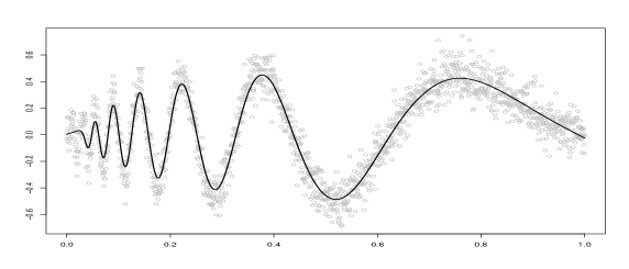
Figure 7: The top panel shows a reconstruction using pspl160 and the bottom panel shows the wss reconstruction for the same data. The sample size is $n=1600.$

The local variability of the bumps data is much more pronounced and the wss estimator outperforms the other estimators in all cases.

5 Heteroscedasticity and robustness

5.1 Nonparametric scale approximations

The ideas developed in the previous section can also be used to obtain nonparametric approximations to heteroscedastic noise. The model we use is

$$Y(t)=\sigma(t)Z(t),\quad 0\leq t\leq 1,$$ (11)

$Z(t)$ Gaussian white noise. Given data $(t_{i},Y(t_{i}))$, $i=1,\dots,n$, we define a confidence region as follows. We define for a function $s:[0,\,1]\rightarrow(0,\infty)$ and an interval $I\subset[0,\,1]$

$$v({\mbox{\boldmath$Y$}}_{n},I,s)=\sum_{t_{i}\in I}Y(t_{i})^{2}/s(t_{i})^{2}$$

and then set

$${\mathcal{C}}_{n}({\mbox{\boldmath$Y$}}_{n},{\mathcal{I}}_{n},\alpha_{n}) = \{s:\text{qu}((1-\alpha_{n})/2,|I|)\leq v({\mbox{\boldmath$Y$}}_{n},I,s)$$

$$\quad\quad\quad\leq\text{qu}((1+\alpha_{n})/2,|I|),\quad I\in{\mathcal{I}}_{n}\}$$

where $\text{qu}(\gamma,k)$ denotes the $\gamma$–quantile of the chi–squared distribution with $k$ degrees of freedom. The rationale is clear. Under the model (11) the $v({\mbox{\boldmath$Y$}}_{n},I,\sigma)$ has the chi–squared distribution with $|I|$ degrees of freedom. By an appropriate choice of $\alpha_{n},$ which may be determined by simulations, ${\mathcal{C}}_{n}({\mbox{\boldmath$Y$}}_{n},{\mathcal{I}}_{n},\alpha_{n})$ is an $\alpha$–confidence region for $\sigma$:

$$P(\sigma\in{\mathcal{C}}_{n}({\mbox{\boldmath$Y$}}_{n},{\mathcal{I}}_{n},\alpha_{n}))=\alpha$$

so that the confidence region is uniform, exact and non-asymptotic. Furthermore in this particular model there are no “nuisance” parameters corresponding to the $\sigma$ of model (3). The default value of $\gamma_{n}$ we use is

$$\gamma_{n}=1-\exp(-1.5\log(n))=1-n^{-1.5}$$

which roughly corresponds to the default choice of $\tau_{n}=3$ in the definition of ${\mathcal{A}}_{n}.$ As before the second step is to regularize in ${\mathcal{C}}_{n}({\mbox{\boldmath$Y$}}_{n},{\mathcal{I}}_{n},\alpha_{n}).$ One possibility which is useful for quantifying the changes in volatility of financial data, the volatility of the volatility, is to take $s$ to be piecewise constant and to minimize the number of intervals of constancy (see Davies, (2006)). In the present context however we are looking for a smooth approximation and we take recourse to weighted smoothing splines. We take $s=s_{n}$ to be the solution of

$$\min\quad\sum_{i=1}^{n}\lambda_{i}(|y_{i}|-s_{n}(t_{i}))^{2}+\int_{0}^{1}s_{n}^{(2)}(t)^{2}\,dt.$$

where again the local weights are data dependent and are chosen so that the solution $s_{n}$ lies in ${\mathcal{C}}_{n}({\mbox{\boldmath$Y$}}_{n},{\mathcal{I}}_{n},\alpha_{n}).$ The procedure we use is similar to that described in Section 3.1 but with some modifications. On intervals $I$ where the inequality

$$\text{qu}((1-\alpha_{n})/2,|I|)\leq v({\mbox{\boldmath$y$}}_{n},I,s_{n})\leq\text{qu}((1+\alpha_{n})/2,|I|)$$ (12)

is not satisfied we increase the weights by a factor of $q$ but we do this firstly for single observations, that is intervals of length one. When (12) is satisfied for all such intervals we consider intervals of length two. When again all the inequalities are satisfied we move on to the next longer intervals until finally all inequalities are satisfied. A similar procedure was used in Davies and Kovac, (2004) in the context of approximating spectral densities. Figure 8 shows the result of the procedure applied to data generated according to the model

$$Y(t)=\sin(4\pi t)^{2}Z(t).$$

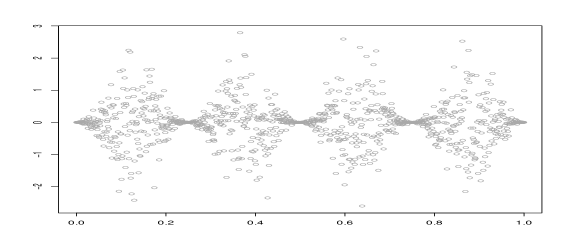
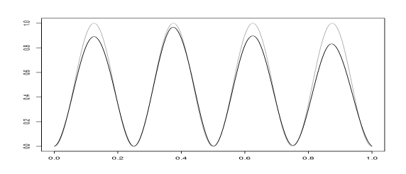
Figure 8: Top panel: heteroscedastic noise. Bottom panel: the scale function and its reconstruction using weighted smoothing spline..

5.2 Robust smoothing

A complete robustification of the procedure described in Section 3.1 would entail replacing (2) by, for example,

$$\min S(g,{\mbox{\boldmath$\lambda$}}):=\sum_{i=1}^{n}\lambda_{i}|y(t_{i})-g(t_{i})|+\int_{0}^{1}g^{(2)}(t)^{2}\,dt,$$

and the definition of approximation (4) by

$${\tilde{w}}({\mbox{\boldmath$y$}}_{n},I,g)=\frac{1}{\sqrt{|I|}}\,\sum_{t_{i}\in I}\text{sgn}(r({\mbox{\boldmath$y$}}_{n},t_{i},g))$$

to give rise to the confidence region

$${\mathcal{D}}_{n}({\mbox{\boldmath$y$}}_{n},{\mathcal{I}}_{n})=\big{\{}g:\max_{I\in{\mathcal{I}}_{n}}\,{\tilde{w}}({\mbox{\boldmath$y$}}_{n},I,g)\leq\sqrt{2\log n\,}\,\big{\}}$$

(see Dümbgen and Kovac, (2005)). A much simpler but reasonably effective method is the following. The noise level $\sigma_{n}$ is quantified by (8). A running median with a window width of say five observations is applied to the data

$$m_{5}(t_{i}):=\text{MED}(y(t_{i-2}),y(t_{i-1}),y(t_{i}),y(t_{i+1}),y(t_{i+2}))$$

and any data point $y(t_{i})$ for which

$$|y(t_{i})-m_{5}(t_{i})|\geq 3.5\sigma_{n},$$

is replaced by $m_{5}(t_{i})$ (see Hampel, (1985)). The weighted splines procedure is now applied to the cleaned data set. The procedure will work well as long as no group of five successive observations contains more than two outliers. Figure 9 shows the result of applying this robustified procedure to a sine curve contaminated with Cauchy noise.

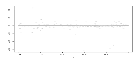
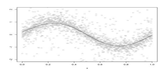
Figure 9: The robustified weighted spline procedure applied to a sine curve contaminated with Cauchy noise

6 Image analysis and weighted thin plate smoothing splines

6.1 Weighted thin plate smoothing splines

We consider data ${\mbox{\boldmath$y$}}_{n}=\{({\mbox{\boldmath$t$}}_{i},y({\mbox{\boldmath$t$}}_{i})):\,i=1,\ldots,n^{2}\,\}$ with the ${\mbox{\boldmath$t$}}_{i}$ of the form

$${\mbox{\boldmath$t$}}_{i}=(j_{i}/n,k_{i}/n),\quad j_{i},k_{i}=0,\ldots,n-1.$$

Corresponding to (2) we consider minimizing

$$S(f,{\mbox{\boldmath$\lambda$}}):=\sum_{i=1}^{n^{2}}\lambda({\mbox{\boldmath$t$}}_{i})(y({\mbox{\boldmath$t$}_{i}})-f({\mbox{\boldmath$t$}_{i}}))^{2}+J(f)$$

with

$$J(f)=\int_{0}^{1}\int_{0}^{1}\left(\left(\frac{\partial^{2}f}{\partial^{2}s}\right)^{2}+2\left(\frac{\partial^{2}f}{\partial s\partial t}\right)^{2}+\left(\frac{\partial^{2}f}{\partial^{2}t}\right)^{2}\right)dsdt$$

It can be shown that the solution is a natural thin plate spline. We refer to Green and Silverman, (1994).

6.2 Approximation in two dimensions

For a given function $g:[0,\,1]^{2}\rightarrow\mathbb{R}$ and a family ${\mathcal{G}}_{n}$ of subsets $G$ of $[0,\,1]^{2}$ we define

$$w({\mbox{\boldmath$y$}}_{n},G,g)=\frac{1}{\sqrt{|G|}}\,\sum_{{\mbox{\boldmath$t$}}_{i}\in G}(y_{n}({\mbox{\boldmath$t$}}_{i})-g({\mbox{\boldmath$t$}}_{i})).$$

For data generated by the model

$$Y({\mbox{\boldmath$t$}})=f({\mbox{\boldmath$t$}})+\sigma Z({\mbox{\boldmath$t$}}),\quad{\mbox{\boldmath$t$}}\in[0,\,1]^{2}$$

this leads to the confidence region

$${\mathcal{H}}^{*}({\mbox{\boldmath$Y$}}_{n},{\mathcal{G}}_{n},\tau)$$

$$= \{g:\max_{G\in{\mathcal{G}}_{n}}\,|w({\mbox{\boldmath$Y$}}_{n},G,g)|\leq\sigma_{n}\sqrt{2\tau\log(n)}\,\}.$$

The additional factor 2 is due to the fact that we now have $n^{2}$ observations. The noise level $\sigma_{n}$ is defined by

$$\sigma_{n} = \frac{1.48}{2}\text{MED}\Big{(}\big{\{}\big{|}y(\textstyle\frac{j_{i}+1}{n},\frac{k_{i}+1}{n})-y(\frac{j_{i}+1}{n},\frac{k_{i}}{n})$$

$$-y(\frac{j_{i}}{n},\frac{k_{i}+1}{n})+y(\frac{j_{i}}{n},\frac{k_{i}}{n})\big{|}:i=1,\dots,n^{2}\big{\}}\Big{)}.$$

The quality of the results depends on the choice of ${\mathcal{G}}_{n}$. If ${\mathcal{G}}_{n}$ contains too few sets then the concept of approximation is too crude. Consequently we require a fine division of $[0,\,1]^{2}$ but one which allows the $w({\mbox{\boldmath$y$}}_{n},G,g)$ to be efficiently calculated. Work in this direction has been done and we refer to Friedrich et al., (2007). The family ${\mathcal{G}}_{n}$ we use is the set of all squares.

6.3 An example

As a simple example we consider the function $F:\mathbb{R}^{2}\rightarrow\mathbb{R}$

$$F(x,y)=10\exp(-x^{2}-2y^{2})$$

on a $50\times 50$ grid on $[-7,4]^{2}$ with added normal noise, $\varepsilon_{i}\sim N(0,1).$ Figure 10 shows the function $F$ and its contaminated version together with the thin plate splines reconstruction using generalized cross-validation and the weighted smoothing spline method. The main drawback of weighted thin plate splines is the numerical difficulty of calculating them for larger grids.

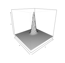
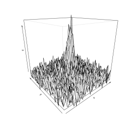
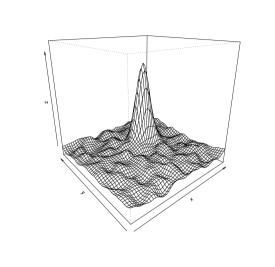
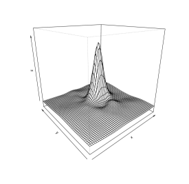
Figure 10: Top row: original function (left) and the noisy data (right). Bottom row: thin plate approximation using GCV (left) and the automatically weighted version (right).

7 Asymptotics

7.1 Weighted smoothing splines

Weighted smoothing splines may be seen as a heuristic method for solving

$$\min\,R(g)\quad\text{ s.~{}t.}\quad g\in{\mathcal{A}}({\mbox{\boldmath$Y$}}_{n},\sigma_{n},{\mathcal{I}}_{n},\tau_{n}).$$ (13)

The resulting function $f_{n}$ is defined by an algorithm and in the absence of a proof that it yields at least an approximate solution, that is

$$\int_{0}^{1}f_{n}^{(2)}(t)^{2}\,dt\leq\,K\min_{g\in{\mathcal{A}}({\mbox{\boldmath$Y$}}_{n},\sigma_{n},{\mathcal{I}}_{n},\tau_{n})}\,\int_{0}^{1}g^{(2)}(t)^{2}\,dt$$

for some constant $K>0,$ we can either establish a rate of convergence on this assumption or we can try and analyse the algorithm. In the first case we are lead to a rate of convergence in the supremum norm of order $(\log(n)/n)^{3/8}.$ Analysing the algorithm as it stands would essentially involve proving that it solves the minimization problem at least approximately. We therefore analyse a modified version of the procedure. We assume that the design points are of the form $t_{i}=i/n$ and that the data are generated as in (3) with

$$f^{(1)}(t)-f^{(1)}(0) = \int_{0}^{t}f^{(2)}(u)\,du,$$ (14)

$$\int_{0}^{1}f^{(2)}(u)^{2}\,du < \infty.$$ (15)

For a given function $g$ we denote the vector of values of $g$ at the design points by ${\mbox{\boldmath$g$}}_{n}.$ We consider firstly the case of a global $\lambda$ and denote the solution of (2) with $\lambda_{1}=\ldots=\lambda_{n}=\lambda$ by ${\mbox{\boldmath$\tilde{f}$}}_{n}(\lambda).$ It can be shown that ${\mbox{\boldmath$\tilde{f}$}}_{n}(\lambda)$ is a solution of

$$\min\quad S_{\lambda}({\mbox{\boldmath$g$}}_{n}):=\sum_{i=1}^{n}\lambda(Y(t_{i})-g_{n}(t_{i}))^{2}+{\mbox{\boldmath$g$}}_{n}^{t}\Omega_{n}{\mbox{\boldmath$g$}}_{n}$$ (16)

where $\Omega_{n}$ is an $n\times n$-non-negative definite matrix with normalized eigenvectors ${\mbox{\boldmath$e$}}_{ni}$ and corresponding eigenvalues $\gamma_{ni},1\leq i\leq n$ with $\gamma_{n1}=\gamma_{n2}=0.$ The remaining eigenvalues satisfy the inequalities

$$c_{1}\frac{i^{4}}{n}\,\leq\,\gamma_{ni}\,\leq c_{2}\frac{i^{4}}{n},\quad 3\leq i\leq n$$ (17)

with the constants $c_{1}$ and $c_{2}$ being independent of $n$ (see Utreras, (1983)). For an interval ${\tilde{J}}\subset\{1,\ldots,n\}$ we denote by $\theta_{I}$ the vector whose elements $\theta_{i}$ are $1/\sqrt{|{\tilde{J}}|}$ for $i\in{\tilde{J}}$ and 0 otherwise. We see that $\|\theta_{I}\|=1$ and for the solution ${\mbox{\boldmath$\tilde{f}$}}_{n}(\lambda)$ of (16) the $w({\mbox{\boldmath$Y$}}_{n},I,{\tilde{f}}_{n}(\lambda))$ of (4) are given by

$$w({\mbox{\boldmath$Y$}}_{n},I,{\tilde{f}}_{n}(\lambda))=\theta_{{\tilde{J}}(I)}I^{t}({\mbox{\boldmath$Y$}}_{n}-{\tilde{\mbox{\boldmath$f$}}}_{n}(\lambda)),\quad I\in{\mathcal{I}}_{n}$$

where ${\tilde{J}}(I)$ is the interval of $\{1,\ldots,n\}$ which gives the indices $i$ with $t_{i}\in I.$ We have

Theorem 7.1

• ${\tilde{\mbox{\boldmath$f$}}}_{n}^{t}(\lambda)\Omega_{n}{\tilde{\mbox{\boldmath$f$}}}_{n}(\lambda)$ is an increasing function of $\lambda.$

• $\mathbb{E}\left({\tilde{\mbox{\boldmath$f$}}}_{n}^{t}(\lambda)\Omega_{n}{\tilde{\mbox{\boldmath$f$}}}_{n}(\lambda)\right)\leq cn^{1/4}\lambda^{5/4}$ for some constant $c.$

• There exists a constant $A>0$ such that for all $\lambda>A/\log n$ and for all ${\mathcal{I}}_{n}$ with $|{\mathcal{I}}_{n}|\leq qn$ for some fixed $q$ and for all $\tau>2$ we have

  $$\lim_{n\rightarrow\infty}\mathbb{P}\big{(}\max_{I\in{\mathcal{I}}_{n}}|w({\mbox{\boldmath$Y$}}_{n},I,{\tilde{f}}_{n}(\lambda))|\leq\sigma\sqrt{\tau\log n\,}\,\big{)}=1.$$

Proof. (a) In the following $I_{n}$ denotes the identity matrix. The solution ${\tilde{\mbox{\boldmath$f$}}}_{n}(\lambda)$ of (16) is given by

$${\tilde{\mbox{\boldmath$f$}}}_{n}(\lambda)=\lambda(\lambda I_{n}+\Omega_{n})^{-1}{\mbox{\boldmath$Y$}}_{n}$$

and on writing ${\mbox{\boldmath$Y$}}_{n}=\sum_{i=1}^{n}\eta_{ni}{\mbox{\boldmath$e$}}_{ni}$ we obtain

$${\tilde{\mbox{\boldmath$f$}}}_{n}^{t}(\lambda)\Omega_{n}{\tilde{\mbox{\boldmath$f$}}}_{n}(\lambda)=\lambda^{2}\sum_{i=3}^{n}\frac{\eta_{ni}^{2}\gamma_{ni}}{(\lambda+\gamma_{ni})^{2}}$$

from which the claim follows on noting that $\gamma_{ni}>0$ for $i\geq 3.$
 
(b) We have

$${\tilde{\mbox{\boldmath$f$}}}_{n}^{t}(\lambda)\Omega_{n}{\tilde{\mbox{\boldmath$f$}}}_{n}(\lambda)=\lambda^{2}{\mbox{\boldmath$Y$}}_{n}^{t}(\lambda I_{n}+\Omega_{n})^{-1}\Omega_{n}(\lambda I_{n}+\Omega_{n})^{-1}{\mbox{\boldmath$Y$}}_{n}$$

and hence

$$\mathbb{E}\left({\tilde{\mbox{\boldmath$f$}}}_{n}^{t}(\lambda)\Omega_{n}{\tilde{\mbox{\boldmath$f$}}}_{n}(\lambda)\right)$$

$$= \lambda^{2}{\mbox{\boldmath$f$}}_{n}^{t}(\lambda I_{n}+\Omega_{n})^{-1}\Omega_{n}(\lambda I_{n}+\Omega_{n})^{-1}{\mbox{\boldmath$f$}}_{n}$$

$$+\sigma^{2}\mathbb{E}\left(\lambda^{2}{\mbox{\boldmath$Z$}}_{n}^{t}(\lambda I_{n}+\Omega_{n})^{-1}\Omega_{n}(\lambda I_{n}+\Omega_{n})^{-1}{\mbox{\boldmath$Z$}}_{n}\right).$$

Arguing as above we obtain

$$\lambda^{2}{\mbox{\boldmath$f$}}_{n}^{t}(\lambda I_{n}+\Omega_{n})^{-1}\Omega_{n}(\lambda I_{n}+\Omega_{n})^{-1}{\mbox{\boldmath$f$}}_{n}$$

$$=\lambda^{2}\sum_{3}^{n}\alpha_{ni}^{2}\frac{\gamma_{ni}}{(\lambda+\gamma_{ni})^{2}}$$

$$\leq\sum_{3}^{n}\alpha_{ni}^{2}\gamma_{ni}={\mbox{\boldmath$f$}}_{n}^{t}\Omega{\mbox{\boldmath$f$}}_{n}$$

and

$$\mathbb{E}(\lambda^{2}{\mbox{\boldmath$Z$}}_{n}^{t}(\lambda I_{n}+\Omega_{n})^{-1}\Omega_{n}(\lambda I_{n}+\Omega_{n})^{-1}{\mbox{\boldmath$Z$}}_{n})$$

$$=\lambda^{2}\sum_{3}^{n}\frac{\gamma_{ni}}{(\lambda+\gamma_{ni})^{2}}.$$

On splitting the last sum into two parts, from $i=3$ to $i=n^{1/4}\lambda^{1/4}$ and from $i=n^{1/4}\lambda^{1/4}$ to $i=n$ and on using (17) we see that

$$\mathbb{E}(\lambda^{2}{\mbox{\boldmath$Z$}}_{n}^{t}(\lambda I_{n}+\Omega_{n})^{-1}\Omega_{n}(\lambda I_{n}+\Omega_{n})^{-1}{\mbox{\boldmath$Z$}}_{n})\leq cn^{1/4}\lambda^{5/4}$$

for some constant $c.$  
(c) We have

$${\mbox{\boldmath$Y$}}_{n}-{\tilde{\mbox{\boldmath$f$}}}_{n}(\lambda)=(\lambda I_{n}+\Omega_{n})^{-1}\Omega_{n}{\mbox{\boldmath$Y$}}_{n}.$$

and on writing ${\mbox{\boldmath$Y$}}_{n}={\mbox{\boldmath$f$}}_{n}+{\mbox{\boldmath$Z$}}_{n}$ we obtain

$${\mbox{\boldmath$Y$}}_{n}-{\tilde{\mbox{\boldmath$f$}}}_{n}(\lambda)={\mbox{\boldmath$h$}}_{n}+\delta_{n}$$

with

$${\mbox{\boldmath$h$}}_{n} = (\lambda I_{n}+\Omega_{n})^{-1}\Omega_{n}{\mbox{\boldmath$f$}}_{n},$$

$$\delta_{n} = \sigma(\lambda I_{n}+\Omega_{n})^{-1}\Omega_{n}{\mbox{\boldmath$Z$}}_{n}.$$

On writing ${\mbox{\boldmath$f$}}_{n}=\sum_{1}^{n}\alpha_{ni}{\mbox{\boldmath$e$}}_{ni}$ we obtain

$${\mbox{\boldmath$h$}}_{n}=\sum_{3}^{n}\alpha_{ni}\frac{\gamma_{ni}}{(\lambda+\gamma_{ni})}{\mbox{\boldmath$e$}}_{ni}$$

and hence

$$\|{\mbox{\boldmath$h$}}_{n}\|^{2} = \sum_{3}^{n}\alpha_{ni}^{2}\frac{\gamma_{ni}^{2}}{(\lambda+\gamma_{ni})^{2}}$$

$$= \frac{1}{\lambda}\sum_{3}^{n}\alpha_{ni}^{2}\frac{\gamma_{ni}^{2}/\lambda}{(1+\gamma_{ni}/\lambda)^{2}}\leq\frac{1}{\lambda}\sum_{3}^{n}\alpha_{ni}^{2}\gamma_{ni}.$$

As ${\mbox{\boldmath$f$}}_{n}^{t}\Omega_{n}{\mbox{\boldmath$f$}}_{n}=\sum_{3}^{n}\alpha_{ni}^{2}\gamma_{ni}$ we see that at least asymptotically

$$\|{\mbox{\boldmath$h$}}_{n}\|^{2}\leq\frac{1}{\lambda}{\mbox{\boldmath$f$}}_{n}^{t}\Omega_{n}{\mbox{\boldmath$f$}}_{n}.$$

We turn to $\delta_{n}.$ We write ${\mbox{\boldmath$Z$}}_{n}=\sum_{1}^{n}Z_{ni}^{*}{\mbox{\boldmath$e$}}_{ni}$ where, because of the transformation is orthonormal, the $Z_{ni}^{*}$ are i.i.d. standard Gaussian random variables. It follows

$$\delta_{n}=\sigma\sum_{3}^{n}Z_{ni}^{*}\frac{\gamma_{ni}}{(\lambda+\gamma_{ni})}{\mbox{\boldmath$e$}}_{ni}$$

and on writing $\theta_{I}=\sum_{1}^{n}\theta_{ni}{\mbox{\boldmath$e$}}_{ni}$ we obtain

$$\mathbb{E}((\theta_{I}^{t}\delta_{n})^{2})=\sigma^{2}\sum_{3}^{n}\theta_{ni}^{2}\left(\frac{\gamma_{ni}}{\lambda+\gamma_{ni}}\right)^{2}\leq\sigma^{2}.$$

The claim of the theorem follows from the usual upper bound for the tail of a Gaussian distribution. $\Box$

We consider the following modified procedure. We consider the solutions ${\tilde{\mbox{\boldmath$f$}}}_{n}(\lambda)$ of (16) and determine the smallest value of $\lambda$ for which ${\tilde{f}}_{n}(\lambda)\in{\mathcal{A}}({\mbox{\boldmath$Y$}}_{n},{\mathcal{I}}_{n},\tau_{n}).$ It follows from (c) of Theorem 7.1 this smallest value is asymptotically with arbitrarily large probability smaller $A/\log n.$ If we denote this solution by ${\mbox{\boldmath$\tilde{f}$}}_{n}(\lambda^{*}_{n})$ then (a) and (b) of Theorem 7.1 imply

$$\lim_{c\rightarrow\infty}\lim_{n\rightarrow\infty}\mathbb{P}\Big{(}{\tilde{\mbox{\boldmath$f$}}}_{n}(\lambda^{*}_{n})^{t}\Omega_{n}{\tilde{\mbox{\boldmath$f$}}}_{n}(\lambda^{*}_{n})\leq cn^{1/4}(\log n)^{-5/4}\Big{)}=1.$$ (18)

for some $c>0.$ Let ${\tilde{\mbox{\boldmath$f$}}}_{n}({\mbox{\boldmath$\lambda$}})$ be the solution obtained from the weighted smoothing spline procedures as described in Section 3.1 respectively. If

$${\tilde{\mbox{\boldmath$f$}}}_{n}({\mbox{\boldmath$\lambda$}})^{t}\Omega_{n}{\tilde{\mbox{\boldmath$f$}}}_{n}({\mbox{\boldmath$\lambda$}})\leq{\tilde{\mbox{\boldmath$f$}}}_{n}(\lambda^{*}_{n})^{t}\Omega_{n}{\tilde{\mbox{\boldmath$f$}}}_{n}(\lambda^{*}_{n})$$

then we accept ${\tilde{\mbox{\boldmath$f$}}}_{n}({\mbox{\boldmath$\lambda$}})$ and otherwise we accept ${\tilde{\mbox{\boldmath$f$}}}_{n}(\lambda^{*}_{n})$ and denote the solution by ${\mbox{\boldmath$f$}}_{n}^{*}.$ We have

Theorem 7.2

If $f$ satisfies (14) and (15) and if $\delta_{n}$ is such that

$$\lim_{n\rightarrow\infty}\delta_{n}n^{5/16}(\log n)^{-9/16}=\infty$$

then

$$\sup_{\delta_{n}\leq t\leq 1-\delta_{n}}|f_{n}^{*}(t)-f(t)|=\text{O}_{P}((\log n)^{7/32}n^{-11/32}).$$

Proof. For a function $g$ satisfying the conditions (14) and (15) we have

$$g(t+s)-g(t) = \int_{0}^{s}g^{(1)}(t+u)\,du=sg^{(1)}(t)+\int_{0}^{s}(g^{(1)}(t+u)-g^{(1)}(t))\,du$$

$$= sg^{(1)}(t)+\int_{0}^{s}\left(\int_{0}^{u}g^{(2)}(t+v)\,dv\right)\,du$$

and hence

$$|g(t+s)-g(t)-sg^{(1)}(t)|\leq\int_{0}^{s}\left(\int_{0}^{u}|g^{(2)}(t+v)|\,dv\right)\,du.$$

As

$$\left(\int_{0}^{u}|g^{(2)}(t+v)|\,dv\right)^{2} = \left(\int_{0}^{1}\{v\leq u\}|g^{(2)}(t+v)|\,dv\right)^{2}$$

$$\leq \int_{0}^{1}\{v\leq u\}^{2}\,dv\int_{0}^{1}g^{(2)}(t)^{2}\,dv=u\int_{0}^{1}g^{(2)}(t)^{2}\,dv$$

for $u$ with $t+u<1$ by Cauchy-Schwarz we obtain

$$|g(t+s)-g(t)-sg^{(1)}(t)| \leq \int_{0}^{s}u^{1/2}\left(\int_{0}^{1}g^{(2)}(t)^{2}\,dv\right)^{1/2}\,du$$

$$= \frac{2}{3}s^{3/2}\left(\int_{0}^{1}g^{(2)}(t)^{2}\,dv\right)^{1/2}.$$

On combining this with the corresponding inequality for $|g(t-s)-g(t)+sg^{(1)}(t)|$ we conclude

$$|g(t+s)+g(t-s)-2g(t)|\leq\frac{4}{3}s^{3/2}\Big{(}\int_{0}^{1}g^{(2)}(u)^{2}\,du\Big{)}^{1/2}$$ (19)

At this point to simplify the proof we assume that ${\mathcal{I}}_{n}$ is the family of all intervals of the form $[t_{i},t_{j}].$ The only effect of taking ${\mathcal{I}}_{n}$ to be the dyadic set of intervals is that the constants in the estimates below are somewhat larger. Consider now point $t_{j}=j/n$ and the interval $I_{j,k}=[t_{j-k},t_{j+k}].$ As $f^{*}_{n}$ lies in ${\mathcal{I}}_{n}$ we have

$$\frac{1}{\sqrt{2k+1}}\Big{|}\sum_{i=-k}^{k}\left(f_{n}^{*}\left(\frac{j+i}{n}\right)-f\left(\frac{j+i}{n}\right)\right)\Big{|}\leq\sigma_{n}\sqrt{\tau_{n}\log n}.$$ (20)

We intend to use (19) with $g=g_{n}=f_{n}^{*}-f$, $t=j/n$ and $s=i/n$. Firstly we note that for this $g$ it follows from (15) and (18) that

$$\int_{0}^{1}g^{(2)}(t)^{2}\,dv=\text{O}_{P}\left(n^{1/4}(\log n)^{-5/4}\right).$$

From this and (19) we deduce

$$f_{n}^{*}\left(\frac{j+i}{n}\right)+f_{n}^{*}\left(\frac{j-i}{n}\right)-f\left(\frac{j+i}{n}\right)-f\left(\frac{j-i}{n}\right)=2\left(f_{n}^{*}\left(\frac{j}{n}\right)-f\left(\frac{j}{n}\right)\right)$$

$$\hskip 341.43306pt+\,R_{n}$$

with

$$R_{n}=\left(\frac{i}{n}\right)^{3/2}\text{O}_{P}\left(n^{1/8}(\log n)^{-5/8}\right).$$

On using this in (20) we obtain after a short calculation

$$\left|f_{n}^{*}\left(\frac{j}{n}\right)-f\left(\frac{j}{n}\right)\right|\leq\left(\frac{k}{n}\right)^{3/2}\text{O}_{P}\left(n^{1/8}(\log n)^{-5/8}\right)+\sigma_{n}\sqrt{\frac{\tau_{n}\log n}{2k}}.$$

As $f$ is continuous it is easy to prove that $\lim_{n\rightarrow\infty}\sigma_{n}=\sigma$ and as, as already noted, $\lim_{n\rightarrow\infty}\tau_{n}=2$ we deduce

$$\left|f_{n}^{*}\left(\frac{j}{n}\right)-f\left(\frac{j}{n}\right)\right|\leq\text{O}_{P}\left(\left(\frac{k}{n}\right)^{3/2}n^{1/8}(\log n)^{-5/8}+\sqrt{\frac{\log n}{k}}\,\right).$$

The result follows on choosing $k=n^{11/16}(\log n)^{9/16}$. $\Box$

We note that for the solution ${\hat{f}}_{n}$ of (13) we have

$$\int_{0}^{1}{\hat{f}}_{n}^{(2)}(t)^{2}\,dt\leq\int_{0}^{1}f^{(2)}(t)^{2}\,dt.$$

This means that we can replace the term $\text{O}_{P}\left(n^{1/8}(\log n)^{-5/8}\right)$ above by $\text{O}_{P}(1).$ The same argument now leads to the rate of convergence $(\log n/n)^{3/8}$ mentioned above.

7.2 Weighted thin plate smoothing splines

The method of prove can be extended to obtain an analogous result for weighted thin plate smoothing splines. As the calculations are somewhat longer we only indicate how to do this. The estimates (17) are replaced by

$$c_{1}\frac{i^{2}}{n}\,\leq\,\gamma_{ni}\,\leq c_{2}\frac{i^{2}}{n},\quad 3\leq i\leq n$$

with the constants $c_{1}$ and $c_{2}$ being independent of $n$ (see Utreras, (1988)). From this the same method of proof used for Theorem 7.1 leads to a corresponding result. The family ${\mathcal{I}}_{n}$ is taken to be the family of squares and now a two-dimensional version of the argument leading to Theorem 7.2 gives the result.

8 Acknowledgments

We gratefully acknowledge the financial support of the Sonderforschungsbereich 475, ‘Komplexitätsreduktion in multivariaten Datenstrukturen’, Department of Statistics, University of Dortmund.

We also acknowledge the helpful comments of an anonymous referee and an Associate Editor which lead to a great improvement in clarity and presentation.

References

- Craven and Wahba, (1978) Craven, P. and Wahba, G. (1978). Smoothing noisy data with spline functions. Estimating the correct degree of smoothing by the method of generalized cross-validation. Numer. Math., 31(4):377–403.
- Davies and Kovac, (2001) Davies, P. and Kovac, A. (2001). Local extremes, runs, strings and multiresolution (with discussion). Annals of Statistics, 29(1):1–65.
- Davies, (1995) Davies, P. L. (1995). Data features. Statistica Neerlandica, 49:185–245.
- Davies, (2006) Davies, P. L. (2006). Long range financial data and model choice. Technical Report 21/06, Collaborative Research Centre 475, Department of Statistics, University of Dortmund, Dortmund, Germany.
- (5) Davies, P. L., Gather, U., and Weinert, H. (2008a). Nonparametric regression as an example of model choice. Communications in Statistics - Simulation and Computation, 37(2). To appear.
- Davies and Kovac, (2004) Davies, P. L. and Kovac, A. (2004). Densities, spectral densities and modality. Annals of Statistics, 32(3):1093–1136.
- (7) Davies, P. L., Kovac, A., and Meise, M. (2008b). Nonparametric regression, confidence regions and regularization. Annals of Statistics, To appear. arXiv:0711.0690[math.ST].
- Denison et al., (1998) Denison, D. G. T., Mallick, B. K., and Smith, A. F. M. (1998). Automatic Bayesian curve fitting. Journal of the Royal Statistical Society, Series B., 60(2):333–350.
- DiMatteo et al., (2001) DiMatteo, I., Genovese, C. R., and Kass, R. E. (2001). Bayesian curve-fitting with free-knot splines. Biometrika, 88(4):1055–1071.
- Donoho and Johnstone, (1995) Donoho, D. L. and Johnstone, I. M. (1995). Adapting to unknown smoothness via wavelet shrinkage. Journal of the American Statistical Association, 90(432):1200–1224.
- Dümbgen, (2003) Dümbgen, L. (2003). Optimal confidence bands for shape-restricted curves. Bernoulli, 9(3):423–449.
- Dümbgen, (2007) Dümbgen, L. (2007). Confidence bands for convex median curves using sign-tests. In Cator, E., Jongbloed, G., Kraaikamp, C., Lopuhaä, R., and Wellner, J., editors, Asymptotics: Particles, Processes and Inverse Problems,, volume 55 of IMS Lecture Notes - Monograph Series 55, pages 85–100, IMS, Haward, USA.
- Dümbgen and Johns, (2004) Dümbgen, L. and Johns, R. (2004). Confidence bands for isotonic median curves using sign-tests. J. Comput. Graph. Statist., 13(2):519–533.
- Dümbgen and Kovac, (2005) Dümbgen, L. and Kovac, A. (2005). Extensions of smoothing via taut strings. Technical report, Institut für mathematische Statistik und Versicherungslehre, University of Bern, Switzerland.
- Dümbgen and Spokoiny, (2001) Dümbgen, L. and Spokoiny, V. (2001). Multiscale testing of qualitative hypotheses. Annals of Statistics, 29(1):124–152.
- Eilers and Marx, (1996) Eilers, P. H. C. and Marx, B. D. (1996). Flexible smoothing with -splines and penalties. Statistical Science, 11(2):89–121. With comments and a rejoinder by the authors.
- Friedrich et al., (2007) Friedrich, F., Demaret, L., Führ, H., and Wicker, K. (2007). Efficient moment computation over polygonal domains with an application to rapid wedgelet approximation. SIAM J. Sci. Comput., 29(2):842–863.
- Green and Silverman, (1994) Green, P. and Silverman, B. (1994). Nonparametric regression and Generalized Linear Models: a roughness penalty approach. Number 58 in Monographs on Statistics and Applied Probabality. Chapman and Hall, London.
- Hampel, (1985) Hampel, F. R. (1985). The breakdown points of the mean combined with some rejection rules. Technometrics, 27:95–107.
- Kabluchko, (2007) Kabluchko, Z. (2007). Extreme-value analysis of standardized gaussian increments. arXiv:0706.1849v2 [math.PR].
- Li, (1989) Li, K.-C. (1989). Honest confidence regions for nonparametric regression. Ann. Statist., 17(3):1001–1008.
- Luo and Wahba, (1997) Luo, Z. and Wahba, G. (1997). Hybrid adaptive splines. Journal of the American Statistical Association, 92:107–116.
- Miyata and Shen, (2003) Miyata, S. and Shen, X. (2003). Adaptive free-knot splines. Journal of Computational and Graphical Statistics, 12:197–213.
- Miyata and Shen, (2005) Miyata, S. and Shen, X. (2005). Free-knot spines and adaptive knot selection. Journal of the Japanese Statistical Society, 35(2):303–324.
- O’Sullivan, (1986) O’Sullivan, F. (1986). A statistical perspective on ill-posed inverse problems. Statistical Science, 1(4):502–527. With comments and a rejoinder by the author.
- O’Sullivan, (1988) O’Sullivan, F. (1988). Fast computation of fully automated log-density and log-hazard estimators. SIAM J. Sci. Statist. Comput., 9(2):363–379.
- Pintore et al., (2006) Pintore, A., Speckman, P., and Holmes, C. C. (2006). Spatially adaptive smoothing splines. Biometrika, 93:113–125.
- Pittman, (2002) Pittman, J. (2002). Adaptrive splines and genetic algorithms. Journal of Computational and Graphical Statistics, 11(3):615–638.
- Ruppert and Carroll, (2000) Ruppert, D. and Carroll, R. (2000). Spacially-adaptive penalties for spline fitting. Australian and New Zealand Journal of Statistics, 42:205–223.
- Ruppert et al., (2003) Ruppert, D., Wand, M. P., and Carroll, R. (2003). Semiparametric Regression. Number 12 in Cambridge Series in Statistical and Probabilistic Mathematics. Cambridge University Press, Cambrisge.
- Utreras, (1983) Utreras, F. I. (1983). Smoothing data under monotonicity constraints: existence, characterization and convergence rates. Zeitung für Numerische Mathematik, 47:611–625.
- Utreras, (1988) Utreras, F. I. (1988). Convergence rates for multivariate smoothing spline functions. Journal of Approximation Theory, 52:1–27.
- Wahba, (1985) Wahba, G. (1985). A comparison of GCV and GML for choosing the smoothing parameter in the generalized spline smoothing problem. Ann. Statist., 13(4):1378–1402.
- Wahba, (1990) Wahba, G. (1990). Spline models for observational data, volume 59 of CBMS-NSF Regional Conference Series in Applied Mathematics. Society for Industrial and Applied Mathematics (SIAM), Philadelphia, PA.
- Wood et al., (2002) Wood, S. A., Jiang, W., and Tanner, M. (2002). Bayesian mixture of splines for spatially adaptive nonparametric regression. Biometrika, 89(3):513–528.
- Zhou and Shen, (2001) Zhou, S. and Shen, X. (2001). Spatially adaptive regression splines and accurate knot selection. Journal of the American Statistical Association, 96:247–259.