Random Cluster Tessellations

Abstract.

This article describes, in elementary terms, a generic approach to produce discrete random tilings and similar random structures by using point process theory. The standard Voronoi and Delone tilings can be constructed in this way. For this purpose, convex polytopes are replaced by their vertex sets. Three explicit constructions are given to illustrate the concept.

1. Introduction

Apart from symmetry and long-range order, also randomness is needed to provide appropriate structure models in physics or chemistry. A well-known example for an application of random points respectively point processes is an ideal gas, which, at each instance of time, may be described by a Poisson point process (cf. [9] p. 449f).

There are also some well-known random tilings with applications in crystallography and material sciences, such as the Poisson Voronoi and the Poisson Delone tessellations ([20, 17]). A more general description of random tilings in the context of quasicrystals can be found in [18, 10]. Recent work of Gummelt [7, 8] is also concerned with establishing a connection between randomness and quasicrystalline structures. Most approaches start from randomly generated points in Euclidean space $\mathbb{R}^{d}$ and then distill the information about the tiles, often convex polytopes, out of the positions of the points. (See Figure 1 for an illustration of this widely used concept.)

Figure 1. A Voronoi tessellation: The (random) points generate their ‘neighbourhoods’

The theory presented in this article is partly based on recent work of Zessin [22], where random tiles are also extracted from random point configurations. However, this approach replaces the concept of convex polytopes by discrete, finite subsets of $\mathbb{R}^{d}$, called clusters. Nevertheless, tilings of convex polytopes can be embedded into this theory by identifying the vertex set of a convex polytope with the polytope itself (see Figure 2). This point of view might describe the underlying structure of the atoms and molecules of certain materials more accurately.

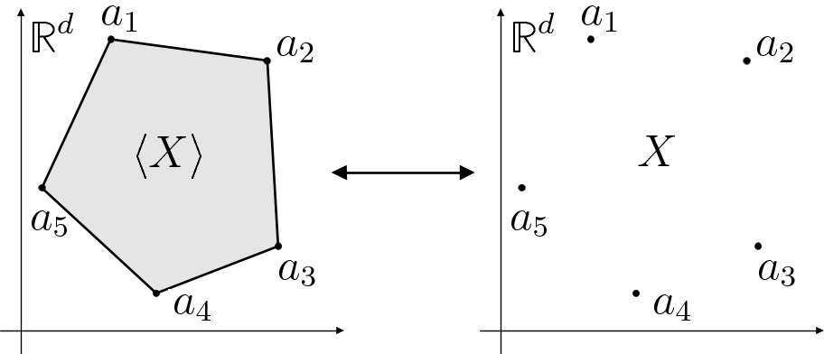
Figure 2. We identify a convex polytope with its vertex set. Here, $\langle X\rangle$ denotes the convex hull of the set $X=\{a_{1},\ldots,a_{5}\}\subseteq\mathbb{R}^{d}$

In this article the desired local and global properties of the tiles, in our case the clusters, enter by means of so called cluster properties. In particular, the first two examples given, are to illustrate this concept. Also, although the examples given in this article are tilings, the presented theory is not restricted to these.

While the typical point processes like the Poisson point process with constant intensity might be ’too random’ to describe condensed matter, this paper gives an explicit example construction to go over to a random tiling ’close’ to a quasicrystalline one.

2. Random Points

Point processes can be constructed in various spaces. Here, we restrict ourselves to random points in $\mathbb{R}^{d}$. See [12] for a more detailed and more general description. To speak about randomness and probabilities, we first need to identify the objects which should be realized randomly. Then we need a notion of which events can be computed or, more precisely, can be given a probability.

Technically, the space for the point configurations is the set of the locally finite simple counting measures in $\mathbb{R}^{d}$, denoted by ${\mathscr{M}^{\bullet}\big{(}\mathbb{R}^{d}\big{)}}$. All possible events are subsumed under the $\sigma$-algebra generated by the counting functions. (A very readable introduction to probability theory and thereby an explanation for the need of terms like measurability and $\sigma$-algebras is given in [6].) A probability measure on ${\mathscr{M}^{\bullet}\big{(}\mathbb{R}^{d}\big{)}}$ equipped with this $\sigma$-algebra is called (simple) point process.

In essence, we can say that the point configurations we want to consider have only finitely many points in every bounded subset of $\mathbb{R}^{d}$, and that the typical events are of the form

$$\left\{\eta\in{\mathscr{M}^{\bullet}\big{(}\mathbb{R}^{d}\big{)}}:\,\eta\text{ has }k\text{ points in }B\right\}\,,$$ (1)

where $B$ is some bounded subset of $\mathbb{R}^{d}$ and $k$ is a non-negative integer. A point process may be viewed as a mechanism to randomly generate point configurations obeying a given probability law. It is comprehensible that the probabilities of those events describe the properties of random point sets in great detail since the bounded sets $B$ in (1) can be chosen arbitrarily small. For calculations, it is very convenient to express a point configuration $\eta$ as a sum of Dirac measures,

$$\eta=\sum_{i=1}^{\infty}\delta_{a_{i}}.$$

Since $\eta$ is assumed to be locally finite, one can always find a suitable sequence $a_{i}$, $i=1,2,\ldots$ of points in $\mathbb{R}^{d}$, e.g., by collecting the points in centred balls of increasing radius and giving them consecutive labels.

An interesting class of point processes are the stationary ones, where the probabilities of the events (1) are invariant under translations of the bounded sets $B$. The best explored class of point processes is the class of Poisson point processes and among them the stationary ones in particular: Let $\lambda\in\mathbb{R}^{+}$ and let $\operatorname{vol}(B)$ denote the volume of a Borel set $B$. The Poisson point process with intensity $\lambda$, $P_{\lambda}$, assigns to our typical events the probabilities

$$P_{\lambda}\left(\left\{\eta\in{\mathscr{M}^{\bullet}\big{(}\mathbb{R}^{d}\big{)}}\text{ has }k\text{ points in }B\right\}\right)=\frac{\left(\lambda\operatorname{vol}(B)\right)^{k}}{k!}\exp\left(-\lambda\operatorname{vol}(B)\right)\,.$$ (2)

The expected number of points in a unit cube thus equals $\lambda$. It is clear that $P_{\lambda}$ is stationary because the probabilities only depend on the translation invariant volume.

In the general case of Poisson point processes, the volume in (2) is replaced by an arbitrary locally finite measure $\rho$ on $\mathbb{R}^{d}$. This results in the Poisson point process with intensity measure $\rho$, denoted by $P_{\rho}$. The process is stationary as long as the intensity measure is translation invariant, which in the case of $\mathbb{R}^{d}$ just means that $P_{\rho}=P_{\lambda}$ for some given $\lambda>0$. For special intensities, it might happen, with positive probability, that point configurations have more than one point in one place. Such situations are excluded if the intensity measure $\rho$ has no pure point part, i.e., if $\rho\left(\{a\}\right)=0$ for all $a\in\mathbb{R}^{d}$. Such point processes are called simple. While $P_{\lambda}$ describes some ideal gas, one might interpret $P_{\rho}$ as gas of non-interacting molecules in a certain physical potential. In contrast to general Gibbs measures (cf. [5]), the particles in the Poissonian case are always non-interacting.

3. Clusters and Cluster Properties

Similar to the above mentioned models for an ideal gas, randomness enters the approach of this paper by means of point point processes, as described in the previous section, where there are a lot of well-known constructions and simulations [21, 20]. But the information one gets out of the typical construction rules are of a more global nature, like distributions. To describe the local properties of the modelled objects and still not to lose the randomness of the point processes, we need a proper concept, which will be described in this section.

As mentioned before, a cluster from our point of view is a finite subset of $\mathbb{R}^{d}$. Let

$$\mathfrak{X}_{d}:=\left\{X\subset\mathbb{R}^{d}\,\big{|}\,\operatorname{card}(X)<+\infty\right\}$$

be the space of clusters in $\mathbb{R}^{d}$ (here $\operatorname{card}(X)$ denotes the cardinality of a set $X$). Typical events in this space are constructed analogously to ${\mathscr{M}^{\bullet}\big{(}\mathbb{R}^{d}\big{)}}$. The method to consider (random) collections of clusters is inspired by the theory of random sets by Matheron [14].

To attach clusters $X\in\mathfrak{X}_{d}$ to point configurations $\eta\in{\mathscr{M}^{\bullet}\big{(}\mathbb{R}^{d}\big{)}}$, we use the concept of cluster properties. A cluster property $\mathscr{D}$ is a measurable (cf. [22] or [15]) subset of the product space $\mathfrak{X}_{d}\times{\mathscr{M}^{\bullet}\big{(}\mathbb{R}^{d}\big{)}}$. The elements $(X,\eta)\in\mathscr{D}$ are the clusters and point configurations which are ‘connected’ in the context of the connection rule $\mathscr{D}$. Although in general misleading, it might be helpful to imagine the (random) points $\eta$ as a set of nuclei, and a connected cluster $X$ as the orbiting electrons of one nucleus, where - of course - not all configurations are possible.

If we take Voronoi and Delone tessellations as typical objects we want to describe, it is easy to see that, for a given point configuration $\eta\in{\mathscr{M}^{\bullet}\big{(}\mathbb{R}^{d}\big{)}}$, we need two concepts for the clusters. In the case of the Voronoi tessellation the vertices of the cells are different from the generating point configuration, while the vertices of the cells in the Delone case coincide with the generating points. To give those concepts a name we will call $X\in\mathfrak{X}_{d}$ a cluster (of Type $\mathscr{D}$) for $\eta$ if just $(X,\eta)\in\mathscr{D}$. If, additionally, $X\subset\eta$ we will call $X$ a cluster in $\eta$. In this notation, the vertices of the Voronoi cells are just clusters for the generating point configurations, while the vertices of the Delone cells are clusters in it. (To stay in the image of nuclei, clusters in a configuration might be imagined as neighboured or even interacting nuclei, where the cluster properties are the interaction rules.)

It can also be convenient to extend the concept of cluster properties to a situation where the clusters and the point configuration do not lie in the same underlying space $\mathbb{R}^{d}$. Therefore we will also consider measurable subsets of $\mathfrak{X}_{d}\times{\mathscr{M}^{\bullet}\big{(}\mathbb{R}^{n}\big{)}}$ as cluster properties, where $d\not=n$. In this context, only clusters for a point configuration are well defined. We will see an example below.

Before we get to more difficult examples and tilings, let us consider a simple cluster property for illustration. Let $r\in\mathbb{R}^{+}$ be fixed. The pair $(X,\eta)$ is defined to belong to the cluster property $\mathscr{D}_{r}\subset\mathfrak{X}_{d}\times{\mathscr{M}^{\bullet}\big{(}\mathbb{R}^{d}\big{)}}$ if $X$ consists of a single point $a_{X}$ and $\eta$ has no point which is closer to $a_{X}$ than $r$ except possibly $a_{X}$, when this is also an element of $\eta$. One cluster of type $\mathscr{D}_{r}$ for a given configuration $\eta$ is easily interpreted as a ball of radius $r$ which does not intersect with the points of $\eta$. But the collection of clusters for $\eta$ has no reasonable interpretation. The collection is also not locally finite in the sense that only finitely many clusters intersect with arbitrary bounded sets of $\mathbb{R}^{d}$. On the other hand, the collection of clusters in $\eta$ is locally finite and can be interpreted as a collection of balls of radius $r/2$ around the points of $\eta$ where all the intersecting balls are removed. Imagine $\eta$ now as a random realization through some point process. Then, the collection of clusters in $\eta$ ‘is’ a random collection of non intersecting balls (see Figure 3).

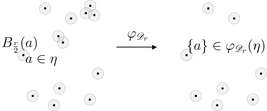
Figure 3. The clusters of type $\mathscr{D}_{r}$ in a point configuration might be interpreted as a collection of non intersecting balls

Note that in the general case, where clusters in or for a point configuration consist of more than one point, the clusters may intersect.

If one wants to examine collections of clusters of certain type for or in random point configurations, it is interesting to know whether the underlying probability law, namely the chosen point process, produces interesting collections of clusters. One indicator for this would be infinitely (but locally finitely) many clusters for almost all point configurations (with respect to the point process). In the case of the clusters in a random configuration, there is the following interesting result from [22]:

$0$-$\infty$-Law of Stochastic Geometry.

Suppose that the cluster property is of the kind that translating a pair $(X,\eta)$ does not alter whether it belongs to the cluster property or not. Let also $P$ be a stationary point process. Then, with probability one, we find either infinitely many clusters in $\eta$ or none.

In the case of the Poisson point process $P_{\lambda}$, and subject to a mild extra assumption (see [22]) one has an even stronger result: Assume that with positive probability there exists at least one cluster in a randomly realized point configuration. This is sufficient to almost always (with respect to $P_{\lambda}$) having infinitely many clusters in such a configuration. Again, it is convenient and possible to express collections, this time not of points but of clusters, by means of Dirac measures. Here, the collection $\varphi_{\mathscr{D}}(\eta)$ of clusters in $\eta$ might be expressed by

$$\varphi_{\mathscr{D}}(\eta) = \sum_{X\text{ is a cluster of type $\mathscr{D}$ in }\eta}\delta_{X}$$ (3)

$$= \sum_{X\subseteq\eta}1_{\mathscr{D}}(X,\eta)\,\delta_{X}\,,$$

where $1_{\mathscr{D}}$ denotes the indicator function of the cluster property $\mathscr{D}$.

Although we do not have the $0$-$\infty$-law in the case of clusters for a configuration, we will see an example where the collection of all the clusters for random $\eta$’s is locally finite. If we combine this function $\varphi_{\mathscr{D}}$ with a point process $P$ (more precisely, we take the image of the point process under the transformation $\varphi_{\mathscr{D}}$), we have a probability measure $\varphi_{\mathscr{D}}(P)$ on cluster configurations (again, see [15] for details). If we see one cluster as a ‘point’ in $\mathfrak{X}_{d}$, the notation ${\mathscr{M}^{\bullet}(\mathfrak{X}_{d})}$ for the (locally finite) cluster configurations is sensible. A probability measure on this spaces is called cluster process.

We will now collect some information about a special family of clusters.

4. Geometry

The cluster configurations of interest for this article are certain discretizations of tilings. Therefore, we need to adopt some well-known concepts of tilings to this case. First we need to define discrete polytopes. Since we want to identify a convex polytope with its vertex set, we take the properties of vertices for the definition: A cluster $X\in\mathfrak{X}_{d}$ is a discrete polytope if, for all points $a\in X$, there exists some hyperplane $H$ such that the intersection of $H$ and the convex hull $\langle X\rangle$ of $X$ consists only of the point $a$. (See Figure 4 for illustration.)

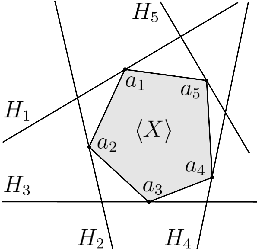
Figure 4. Illustration of a discrete polytope $X=\{a_{1},\ldots,a_{5}\}$ and corresponding supporting hyperplanes $H_{1},\ldots,H_{5}$

It is quite obvious that there exists a one-to-one correspondence between convex and discrete polytopes. The convex polytope is retrieved from a discrete one by taking the convex hull.

Similarly, discrete simplices are obtained. For the construction in the next section, we need a strong property of simplices that is well-known in the $2$-dimensional case: Every triangle has a uniquely defined circumcircle. In higher dimensions, a full-dimensional simplex $\langle X\rangle$ has a uniquely defined circumball $K(X)$ where the complete vertex set – the discrete simplex $X$ – is contained in the border, the circumsphere $S(X)$ (see Figure 5); we refer to [15] for a proof.

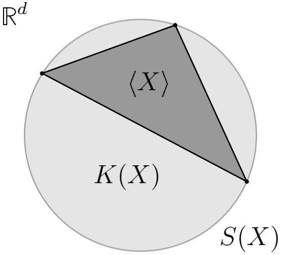
Figure 5. Circumball and circumsphere for a simplex (in this case a triangle)

A collection $\mu\in{\mathscr{M}^{\bullet}(\mathfrak{X}_{d})}$ of discrete polytopes is called a cluster tessellation if the collection of the convex hulls of the clusters form a locally finite face-to-face tiling. In our context ’face-to-face’ does not necessarily mean that there are no holes in the tiling. It just states, that if two tiles intersect, they intersect in whole faces. The collection $\mu$ is called simplicial if all polytopes in it are simplices. It is called complete if the collection of convex hulls covers the whole of $\mathbb{R}^{d}$. If a cluster process is concentrated on the set of cluster tessellations, it is called random cluster tessellation.

5. Examples

In this section, we give three examples for random cluster tessellations, constructed via cluster properties. The first one consists of clusters in a point configuration and the second one of clusters for a point configuration. In both cases, the underlying space for clusters and point configurations is the same, the cluster properties are subsets of $\mathfrak{X}_{d}\times{\mathscr{M}^{\bullet}\big{(}\mathbb{R}^{d}\big{)}}$. In the third example, the point configurations lie in some higher dimensional space, where the underlying space of the clusters can be interpreted as an embedded subspace.

First example: a special Delone tiling

The cluster property that generates our tiling is defined as follows: Let $R\in\mathbb{R}^{+}$ be fixed. For a discrete simplex, let $\dot{K}(X)=:K(X)\smallsetminus X$ denote the circumball of $X$, where the discrete simplex is removed.

A tuple $(X,\eta)\in\mathfrak{X}_{d}\times{\mathscr{M}^{\bullet}\big{(}\mathbb{R}^{d}\big{)}}$ belongs to the cluster property $\mathscr{D}_{R}$ if

1. $X$ is a $d$-dimensional simplex,

2. $\dot{K}(X)$ does not intersect with $\eta$, and

3. $K(X)$ has a radius $\leq R$.

Figures 6 and 7 illustrate clusters of type $\mathscr{D}_{R}$ in a given point configuration $\eta$.

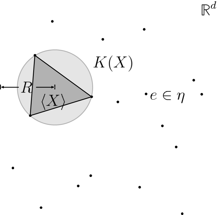
Figure 6. Illustration of clusters of type $\mathscr{D}_{R}$ in a given $\eta$

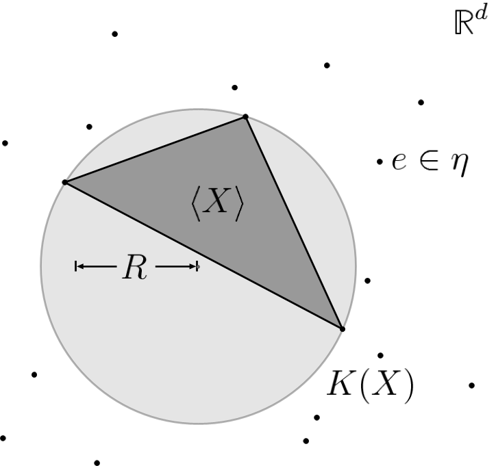
(a) $X$ is not a cluster in $\eta$, because the radius of the circumball is to big

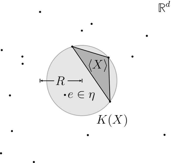
(b) $X$ is a not cluster in $\eta$, because there is another point of the configuration in the circumball

Figure 7. Illustration of clusters that fail to be of type $\mathscr{D}_{R}$ in a given $\eta$

The first two assumptions are based on ideas of Delone [4] and ensure that, for a given $\eta\in{\mathscr{M}^{\bullet}\big{(}\mathbb{R}^{d}\big{)}}$, the cluster configuration

$$\varphi_{\mathscr{D}_{R}}(\eta):=\sum_{X\text{ is a cluster of type $\mathscr{D}_{R}$ in }\eta}\delta_{X}$$ (4)

is face-to-face and simplicial. The assumption (iii) makes the cluster configuration locally finite and thus a tessellation. On the other hand it produces holes in the tessellation (more precisely: in the union of the convex hulls of the clusters) when the points in $\eta$ are not dense enough. (Figure 8 gives a typical section out of such an incomplete tessellation.)

Figure 8. A typical section of a tessellation of the kind of Eq. (4)

Thus, we get the following results:

Proposition 1.

Any simple point process $P$ generates a random tessellation in the form of $\varphi_{\mathscr{D}_{R}}(P)$ as explained in Section 3.

If we again consider the Poisson point process $P_{\lambda}$, we can apply the $0$-$\infty$-law of stochastic geometry to obtain:

Proposition 2.

$P_{\lambda}$-almost surely,

1. there are infinitely many clusters of type $\mathscr{D}_{R}$ in a realization $\eta$, and

2. there are holes in the tessellation.

Here, (ii) holds due to the fact, that a realization of a Poisson point process almost always has arbitrarily big gaps somewhere between the points. This, see [15], could possibly lead to models for random holes in certain condensed matter.

Second example: discrete Voronoi tilings

This example describes a construction of the well-known Poisson Voronoi tiling. In [15], a generalization, so-called random Laguerre tessellations, based on marked point processes and the theory provided by Schlottmann [19], is constructed. However, the idea of random tessellations constructed as clusters for random point configurations is better illustrated in this easier case, so we stick to it.

To understand the generating cluster property, recall the definition of Voronoi cells for a given point configuration $\eta\in{\mathscr{M}^{\bullet}\big{(}\mathbb{R}^{d}\big{)}}$. If $a\in\eta$, the Voronoi cell of $a$ in $\eta$ is given by

$$V_{\eta}(a):=\{v\in\mathbb{R}^{d}\,|\,\text{No other point of }\eta\text{ is closer to }v\text{ than }a\}\,.$$

We call $a$ the center of the Voronoi cell $V_{\eta}(a)$. The definition is illustrated in Figure 9.

Figure 9. The Voronoi cell of $a$ in $\eta=\delta_{a}+\delta_{a_{1}}+\delta_{a_{2}}+\ldots$

If the convex hull of $\eta$ is the whole space $\mathbb{R}^{d}$, the Voronoi cell is a convex polytope.

We can now define our cluster property $\mathscr{D}_{V}$ for this example: $(X,\eta)\in\mathscr{D}_{V}$ if

1. the convex hull of $\eta$ is $\mathbb{R}^{d}$ and

2. $X$ is the vertex set of a Voronoi cell in $\eta$.

In this case, it is easy to see that, for every $\eta\in{\mathscr{M}^{\bullet}\big{(}\mathbb{R}^{d}\big{)}}$, there are no clusters of type $\mathscr{D}_{V}$ in $\eta$. But as long as (i) holds, the collection

$$\psi_{\mathscr{D}_{V}}(\eta):=\sum_{X\text{ is a cluster of type $\mathscr{D}_{V}$ for }\eta}\delta_{X}$$

is a complete cluster tessellation (a proof can be found in [21]). See Figure 10 for an illustration.

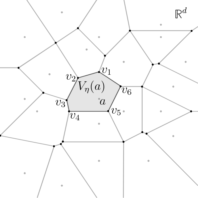
Figure 10. $X=\{v_{1},\ldots,v_{6}\}$ is a cluster of type $\mathscr{D}_{V}$ for the configuration $\eta$ since it is the vertex set of the Voronoi cell $V_{\eta}(a)$

The Poisson point process $P_{\lambda}$ produces point configurations of the kind (i) with probability one. Thus, we have:

Proposition 3.

$\psi_{\mathscr{D}_{V}}(P_{\lambda})$ is a complete random tessellation.

Third example: a random cut and project tiling

This example is based on the so called cut and project scheme, a method to obtain tilings from a (higher dimensional) lattice. The vertices or the centers, in the sense of Voronoi cells, of the tiles are projections of subsets of the lattice. A detailed description of the underlying theory can be found in [16]. A large group of deterministic tilings can be constructed this way, for instance the Penrose Tiling (cf. [3]) or the Ammann-Beenker Tiling (cf. [2]). We present a way to construct random tilings which are ‘close’ to the known deterministic ones, where ‘close’ will have two meanings: in the first one the random points still lie on the lattice but not every point of the lattice will appear. The second interpretation will produce one point for every lattice point, but the points might be randomly shifted within some given radius.

Again, we stick to a simple example, a $1$-dimensional tiling. The mechanisms for randomness can easily be adapted to any tiling that can be obtained via the cut and project scheme. The deterministic case of our example is described in [1].

Consider the $2$-dimensional lattice

$$\varLambda:=\left\{\left(u+v\,\sqrt{2}\,,\,u-v\,\sqrt{2}\right)\middle|\,u,v\text{ integers}\right\}\subset\mathbb{R}^{2}\,.$$

Let $\pi$ be the projection onto the first coordinate and $\pi^{*}$ the one onto the second. Consider the set

$$W:=\left\{e\in\mathbb{R}^{2}\,\middle|\,\pi^{*}(e)\in\left[-\frac{1}{\sqrt{2}},\frac{1}{\sqrt{2}}\right]\right\}\,,$$

which we will call strip. The projection $\pi(\varLambda\cap W)$ forms the vertex set of the so-called silver-mean chain, which is a deterministic aperiodic tiling (again cf.[1]). Figure 11 illustrates this concept.

Figure 11. The projections of the points in $\varLambda\cap W$ form the vertex set of an aperiodic tiling

The appropriate cluster property $\mathscr{D}_{S}\subset\mathfrak{X}_{1}\times{\mathscr{M}^{\bullet}\big{(}\mathbb{R}^{2}\big{)}}$ can be defined as follows: $\left(X,\eta\right)\in\mathscr{D}_{S}$ if and only if

1. $\operatorname{card}X=2$,

2. $X=\{a=\pi(e_{1}),b=\pi(e_{2})\}$, with $e_{1}\not=e_{2}\in\eta\cap W$ and

3. the intersection of the open intervall $(a,b)$ and $\pi(\eta\cap W)$ is empty.

In this $2$-dimensional case, it is easy to see that, as long as $\pi(\eta\cap W)$ is a discrete point set,

$$\psi_{\mathscr{D}_{S}}(\eta):=\sum_{X\text{ is a cluster of type $\mathscr{D}_{S}$ for }\eta}\delta_{X}$$

is a $1$-dimensional tessellation where neighboured points form a cluster, respectively the vertex set of a tile.

To embed the deterministic version of the tiling into point process theory, just define $P_{\varLambda}$ to be the point process in $\mathbb{R}^{2}$ which produces the lattice $\varLambda$ with probability one. Then, $\psi_{\mathscr{D}_{S}}(P_{\varLambda})$ is a process that almost surely produces the silver means tiling. This tiling consists of two prototiles of length $1$, and $1+\sqrt{2}$, respectively.

For the first random version, consider the discrete measure

$$\rho:=\sum_{e\in\varLambda}c\cdot\delta_{e}\,,$$

where $c$ is some positive constant. As mentioned above, $P_{\rho}$, the Poisson point process with intensity measure $\rho$, might produce point configurations with more than one atom in a single point, in this case in the points of $\varLambda$. All the point sets produced by the random mechanism $P_{\rho}$ have the form

$$\eta=\sum_{e\in\varLambda}k_{e}(\eta)\cdot\delta_{e}\,,$$

where $k_{e}(\eta)$ is some natural number or $0$. The support of such an $\eta$ is defined as

$$\operatorname{supp}(\eta):=\sum_{e\in\varLambda,\,k_{e}(\eta)\not=0}\delta_{e}\,.$$

The support is a subset of $\varLambda$, especially has only one atom at every point. Let $P^{*}_{\rho}$ be the image of $P_{\rho}$ under the mapping $\operatorname{supp}$. Thus:

Proposition 4.

$P^{*}_{\rho}$ is again a simple point process, where the realizations are random subsets of the lattice. The probability for a certain point $e$ of $\varLambda$ to be in the random set is $1-\mathrm{e}^{-c}$.

Figure 12 shows a typical randomly realized point set and what happens by taking the cut and project clusters.

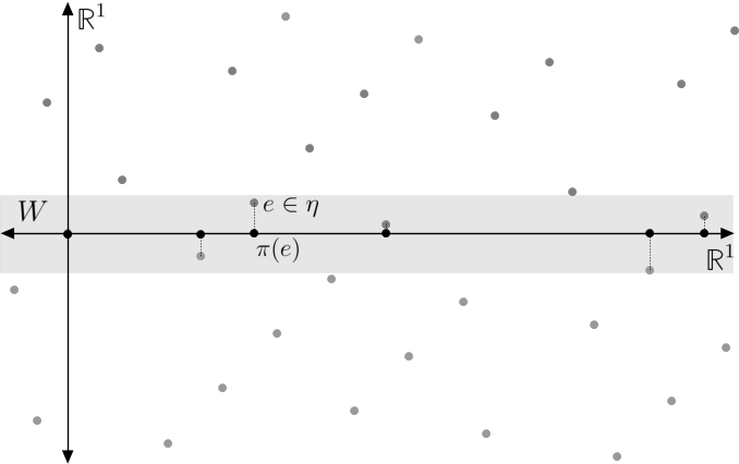
Figure 12. $P_{\rho}^{*}$ produces random subsets of the lattice $\varLambda$, the tiles might become larger

Since the holes in such a random subset cannot be controlled, the tiles corresponding to the clusters for a random $\eta$ might have any length of the form $n+m\sqrt{2}$, $n,m$ non-negative integers.

The next point process randomly shifts the points of the lattice. Another way to randomly shift the points is presented in [11]. There might be some way to transform these two approaches into one another. For the construction of our point process, let $\varepsilon>0$ and $B_{\varepsilon}(e)$ the ball of radius $\varepsilon$ and centre $e$, $e\in\varLambda$. $\varepsilon$ should be choosen small enough so that the balls do not intersect. Consider the mapping $\boldsymbol{b}_{e}:{\mathscr{M}^{\bullet}\big{(}\mathbb{R}^{2}\big{)}}\to{\mathscr{M}^{\bullet}\big{(}\mathbb{R}^{2}\big{)}}$,

$$\boldsymbol{b}_{e}(\eta):=\begin{cases}\frac{1}{\operatorname{card}(\eta\cap B_{\varepsilon}(e))}\sum_{f\in\eta\cap B_{\varepsilon}(e)}f\,,&\text{if }\eta\cap B_{\varepsilon}(e)\not=\emptyset\,,\\ e\,,&\text{if }\eta\cap B_{\varepsilon}(e)=\emptyset\,,\end{cases}$$

which gives the barycentres of all the points in $\eta\cap B_{\varepsilon}(e)$. The configuration

$$\boldsymbol{b}(\eta):=\sum_{e\in\varLambda}\boldsymbol{b}_{e}(\eta)$$

of all these barycentres, by construction, has exactly one point in every $\varepsilon$-ball around the lattice points.

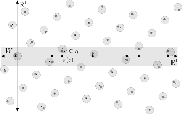
Figure 13. For typical realisations $\eta$ of $P_{\boldsymbol{b}}$ the projections of $\eta\cap W$ form slightly changed tiles or even completely new ones

Thus we have the following result:

Proposition 5.

If you take some arbitrary simple point process $P$, e.g. $P_{\lambda}$, the image $P_{\boldsymbol{b}}$ of $P$ under the mapping $\boldsymbol{b}$ randomly produces point configurations with exactly one point in every $\varepsilon$-ball centred in the lattice points.

Figure 13 illustrates the typical situation and the resulting projections. The corresponding tiles to the clusters for a given $\eta$ typically are close to the tiles of the original silver means tiling, differing in length up to $2\cdot\varepsilon$. But since certain $\varepsilon$-balls of points in $\varLambda\cap W^{\complement}$ intersect with the strip $W$, there might be ‘completely new’ tiles. Nevertheless, the density of the vertices stays the same, since the probabilities to shift a point into and to the outside of the strip are the same.

In both of the cases of the third example of this article, it is easy to see the following:

Proposition 6.

The cluster processes $\psi_{\mathscr{D}_{S}}(P^{*}_{\rho})$, respectively $\psi_{\mathscr{D}_{S}}(P_{\boldsymbol{b}})$, are random $1$-dimensional tessellations.

6. Conclusions

Point processes, especially the Poisson point processes, in combination with cluster properties give access to modelling discrete random structures. The information of the cluster properties in this case carry the information about possible connections respectively interactions of the particles. The third type of example shows a way to slightly randomise aperiodic tilings. In this context, future applications to random tilings in the sense of Gummelt [7, 8] are of interest. If point processes could be constructed that almost surely produce more special configurations, e.g. Delone or FLC (cf. for instance [13]) sets, the presented methods might get closer to applications like glasses or foams.

Acknowledgements

It is a pleasure to thank M. Baake, D. Frettlöh, C. Richard and H. Zessin for several useful comments and clarifying discussions. I also want to thank the reviewers for a number of very helpful suggestions to improve the manuscript.

This work was partially supported by the German Research Council (DFG), within the CRC 701.

References

- [1] M. Baake, U. Grimm and R. V. Moody: What is aperiodic order? Preprint 2002, URL: http://arxiv.org/abs/math.HO/0203252.
- [2] F. P. M. Beenker: Algebraic theory of non-periodic tilings of the plane by two simple building blocks: a square and a rhombus. Eindhoven University of Technology, 1982, TH-Report, 82-WSK04.
- [3] N. G. de Bruijn: Algebraic Theory of Penrose’s Non-Periodic Tilings of the Plane I, II. Nederl. Akad. Wetensch. Proc. Series A 84 (1981) 39–52 and 53–66.
- [4] B. Delone: Sur la sphére vide. Bull. Acad. Sci. URSS 6 (1934) 793–800.
- [5] H.-O. Georgii: Gibbs Measures and Phase Transitions. De Gruyter, Berlin 1988.
- [6] H.-O. Georgii: Stochastik. De Gruyter, Berlin 2004.
- [7] P. Gummelt: Random Cluster Covering Model. Journal of Non-Crystalline Solids 334 & 335 (2004), 62–67.
- [8] P. Gummelt: Decacon Covering Model and Equivalent HBS-Tiling Model. Z. Kristallogr. 221 (2006), 582–588.
- [9] C. V. Heer: Statistical Mechanics, Kinetic Theory and Stochastic Processes. Academic Press, New York 1972.
- [10] C. L. Henley: Random Tiling Models. In: Quasicrystals: The State of the Art, eds. D. P. DiVincenco and P. J. Steinhardt, Series on Condensed Matter Physics, vol. 16, 2nd edition, World Scientific, Singapore, 1999, pp. 459–560.
- [11] A. Hof: Diffraction by aperiodic structures at high temperatures J. Phys. A: Math. Gen. 28 (1995) 57–62.
- [12] J. Kerstan, K. Matthes, and J. Mecke: Infinitely Divisible Point Processes. Wiley, Chichester 1978.
- [13] J.-Y. Lee, R. V. Moody and B. Solomyak: Pure Point Dynamical and Diffraction Spectra. Ann. Henri Poincaré 3 (2002), no. 5, 1003–1018.
- [14] G. Matheron: Random Sets and Integral Geometry. Wiley, New York 1975.
- [15] K. Matzutt: Konstruktionen zufälliger lokal endlicher Mosaike, insbesondere Laguerrescher. Diploma thesis, Fakultät für Mathematik, Universität Bielefeld, 2006.
- [16] R. V. Moody: Meyer Sets and Their Duals. In: The Mathematics of Aperiodic Order, ed. R. V. Moody, Proceedings of the NATO-Advanced Study Institute on Long-range Aperiodic Order, NATO ASI Series C 489, Kluwer, Dordrecht 1997, 403–441.
- [17] A. Okabe, B. Boots, and K. Sugihara: Spatial Tessellations. Wiley, Chichester 1992.
- [18] C. Richard, M. Höffe, J. Hermisson and M. Baake: Random Tilings: Concepts and Examples. J. Phys. A: Math. Gen. 31 (1998) 6385–6408
- [19] M. Schlottmann: Periodic and Quasi-Periodic Laguerre Tilings. Intern. J. Mod. Phys. B 6 & 7 (1993) 1351–1363.
- [20] D. Stoyan, W. S. Kendall, and J. Mecke: Stochastic Geometry and its Applications. 2nd edition, Wiley, Chichester 1995.
- [21] R. Schneider and W. Weil: Stochastische Geometrie. Teubner, Stuttgart 2000.
- [22] H. Zessin: The Gibbs Cluster Process. Preprint, Fakultät für Mathematik, Universität Bielefeld, 2005. URL: http://www.mathematik.uni-bielefeld.de/fsp-math/Preprints/170.pdf.