Effect of confinement potential shape on exchange interaction in coupled quantum dots

Abstract

Exchange interaction has been studied for electrons in coupled quantum dots (QD’s) by a configuration interaction method using confinement potentials with different profiles. The confinement potential has been parametrized by a two-centre power-exponential function, which allows us to investigate various types of QD’s described by either soft or hard potentials of different range. For the soft (Gaussian) confinement potential the exchange energy decreases with increasing interdot distance due to the decreasing interdot tunnelling. For the hard (rectangular-like) confinement potential we have found a non-monotonic behaviour of the exchange interaction as a function of distance between the confinement potential centres. In this case, the exchange interaction energy exhibits a pronounced maximum for the confinement potential profile which corresponds to the nanostructure composed of the small inner QD with a deep potential well embedded in the large outer QD with a shallow potential well. This effect results from the strong localization of electrons in the inner QD, which leads to the large singlet-triplet splitting. Implications of this finding for quantum logic operations have been discussed.

1 Introduction

An exchange interaction between electrons localized in coupled quantum dots (QD’s) is a very promising tool for manipulating qubits in semiconductor nanodevices [1]. This interaction can change the spin of the electron, which allows us to perform the quantum logic operations with spin qubits [1, 2, 3, 4, 5]. Recently, the exchange-interaction induced spin swap operations in coupled QD’s have been simulated by a direct solution of a time-dependent Schődinger equation [6]. The quantum logic operations can be performed in the laterally coupled QD’s [7, 8, 9] and quantum wire QD systems [10, 11]. Conditions of a realization of the logic operations with qubits in QD’s are determined by the properties of electron states in QD nanostructures. The electron states of the laterally coupled QD’s have been studied theoretically in Refs. [12, 13, 14, 15, 16, 17, 18, 19, 20, 21, 22]. In electrostatically gated QD’s [7], the properties of the electron quantum states can be tuned by changing the external voltages applied to the gates [23].

In order to perform the high-fidelity quantum logic operations with spin qubits the exchange interaction should be possibly strong. The exchange interaction energy, defined as the difference between the lowest triplet and singlet energy levels, depends on the localization of electrons in the QD’s. In general, the stronger the electron localization the stronger the exchange coupling. The electron localization is determined by the profile of the potential confining the electrons within the QD’s. Therefore, the exchange interaction depends on the shape and range of the confinement potential. Usually, the confinement potential in coupled QD’s is modelled by the two-centre parabolic [14, 21] or Gaussian [16, 17] potential.

In the present paper, we propose the two-centre power-exponential (PE) potential [24], which allows us to study a broad class of confinement potentials with different shapes. The one-centre PE potential [24] is very well suited for a description of the electrostatic QD’s [23, 25]. It has a form

$$V(r)=-V_{0}\exp[-(r/R)^{p}]\;,$$ (1)

where $V_{0}$ is the depth of the potential well, $R$ is the range of the potential, which determines the QD size, and parameter $p\geq 2$ describes ”a softness” of the potential, i.e., a smoothness of the QD boundaries. If $p\simeq 2$, the potential is ”soft”, and if $p\geq 4$, the potential is ”hard”, i.e., it possesses the walls with large steepness. Parameter $p$ can be used to describe a different steepness of the QD boundaries. Therefore, PE potential (1) can be applied to a modelling of the electrostatically gated QD’s [7, 23] and self-assembled QD’s with compositional modulation [26]. The influence of the smoothed interfaces on the electronic and optical properties of GaAs/$\mathrm{Al_{x}Ga_{1-x}As}$ QD’s have been studied in a recent paper [27].

The exchange interaction can be controlled by internal nanostructure parameters, e.g., size and geometry of the coupled QD’s, and external electric and magnetic fields [16, 17, 20]. It has been shown [16] that the asymmetry of QD’s leads to the increase of this interaction. Recently, the size effects in the exchange coupling have been studied for quantum wire QD systems [11].

In the present paper, we investigate the influence of the shape and range of the confinement potential on the exchange interaction in laterally coupled QD’s using the two-centre PE potential. The paper is organized as follows: a theoretical model is presented in Section II, the calculation methods and results are given in Section III, Section IV includes the discussion and Section V – the conclusions and summary.

2 Theory

We study the system of two electrons confined in laterally coupled QD’s with identical confinement potentials. The geometry of the nanostructure, which consists of two separated QD’s, is illustrated in Figure 1. We describe each QD by the two-dimensional (2D) rotationally symmetric potential well centred at positions $\pm\mathbf{a}$, where $\mathbf{a}=(d/2,0)$ and $d$ is the distance between the centres of the potential wells.

Figure 1: Schematic of the coupled QD system. Circles $A$ and $B$ represent the QD’s, $d$ is the distance between the centres of the confinement potentials, $\mathbf{a}$ is the position vector of the centre of the right QD.

In the effective mass approximation the Hamiltonian of the system reads

$$H=h_{1}+h_{2}+\frac{e^{2}}{4\pi\varepsilon_{0}\varepsilon_{s}r_{12}}\;,$$ (2)

where $h_{j}$ ($j=1,2$) is the one-electron Hamiltonian, $\varepsilon_{0}$ is the electric permittivity of the vacuum, $\varepsilon_{s}$ is the static relative electric permittivity, $r_{12}=|\mathbf{r}_{1}-\mathbf{r}_{2}|$ is the electron-electron distance, and $\mathbf{r}_{j}=(x_{j},y_{j})$ denote the electron position vectors. The one-electron Hamiltonian has the form

$$h_{j}=-\frac{\hbar^{2}}{2m_{e}}\nabla_{j}^{2}+V(\mathbf{r}_{j})\;,$$ (3)

where $m_{e}$ is the electron effective band mass and $V(\mathbf{r}_{j})$ is the confinement potential. We assume that the effective mass and the static electric permittivity do not change across the QD boundaries. This assumption is well justified for the electrostatic QD’s based on GaAs [23]. For the coupled QD’s the confinement potential is taken on as a sum of PE potentials [Eq. (1)] centred at $\pm\mathbf{a}$. In the explicit form,

$$V(\mathbf{r})=-V_{0}\Big{\{}\exp[-(r_{A}/R)^{p}]+\exp[-(r_{B}/R)^{p}]\Big{\}}\;,$$ (4)

where $r_{A}=|\mathbf{r}+\mathbf{a}|$ and $r_{B}=|\mathbf{r}-\mathbf{a}|$.

Formula (4) defines a broad class of two-centre confinement potentials with different shapes. For fixed potential well depth $V_{0}$ and range $R$ parameter $p$ characterizes the softness (hardness) of the confinement potential. The smaller (larger) $p$ the potential is more soft (hard). For $p=2$ the confinement potential has the Gaussian shape. This potential is soft, i.e., the potential walls at the QD boundaries, have fairly small steepness and are partly penetrable for the electron. For $p\geq 4$ the confinement potential becomes hard, i.e., the potential walls at the QD boundaries are steep. For $p\geq 10$ we deal with the rectangular-type, very hard, confinement potential. Figure 2 shows the different profiles of the two-centre confinement potential [Eq. (4)]. In Figure 2 and throughout the present paper we are using the donor Rydberg $R_{D}=m_{e}e^{4}/(32\pi^{2}\varepsilon_{0}^{2}\varepsilon_{s}^{2}\hbar^{2})$ as the unit of energy and the donor Bohr radius $a_{D}=4\pi\varepsilon_{0}\hbar^{2}/(m_{e}e^{2})$ as the unit od length. For GaAs, $R_{D}\simeq 6$ meV and $a_{D}\simeq 10$ nm. We note the essential difference in potential profiles between the soft ($p=2$) and hard ($p=10$) confinement potentials for intermediate distances $d$, i.e., for $d\simeq 3\;a_{D}$ in Figure 2. In the case of soft confinement potential, the resulting two-centre potential changes smoothly with increasing $d$ from the single to the double potential well. In this case, the increasing intercentre distance $d$ leads first to the increase of the potential well size and next to the formation of the potential barrier for $d\geq 3\;a_{D}$. If the confinement potential is hard, then – for intermediate intercentre distances $d$ – we obtain a narrow deep potential well surrounded by fairly wide potential steps, on which the potential is flat [cf. Figures 2(b,c)]. This shape of the confinement potential corresponds to the core-shell QD-nanostructure, which was realized in CdTe/CdS self-assembled QD’s [28]. In this case, we deal with the compound QD nanostructure, which consists of the small inner QD embedded in the larger outer QD.

Figure 2: Confinement potential profile for different distances $d$ between the potential well centres as a function of coordinate $x$. Solid curves correspond to the hard confinement potential ($p=10$), dashed curves correspond to the soft confinement potential ($p=2$). The plots for $V_{0}=25R_{D}$ and $R=2a_{D}$.

3 Results

We are mainly interested in the influence of the shape of the confinement potential, in particular its softness, on the electronic properties of coupled QD’s. Therefore, we have performed the calculations for fixed depth $V_{0}=25\;R_{D}$ and range $R=2\;a_{D}$ (except otherwise specified). These values of the parameters correspond to laterally coupled GaAs QD’s [9].

3.1 One-electron problem

The one-electron eigenvalue problem for the one-centre confinement potential has been solved for the Gaussian potential in Ref. [29] and for the PE potential in Ref. [24]. In the present paper, we consider the one-electron bound states for the two-centre confinement potential (4). We have solved the eigenvalue problem for Hamiltonian (3) by the imaginary time step method [30] applying the finite-difference approximation of Hamiltonian (3) on the 2D grid with $101\times 101$ mesh. In this case, the accuracy of the method [30] is high enough to treat the obtained numerical solutions as exact.

Figure 3 shows the results for the six lowest-energy levels, which correspond to the one-electron states used to a construction of two-electron configurations. Figures 3(a) and 3(b) display the results for the soft ($p=2$) and hard ($p=10$) confinement potential, respectively. For $d=0$ we deal with the single QD with the potential well of double depth ($2V_{0}$), while for large $d$ the QD’s are separated by the potential barrier. For intermediate $d$ the superposition of hard-wall potentials corresponds to the inner-outer QD nanostructure [cf. Figures 2(b) and 2(c)]. These properties of the confinement potentials affect the one-electron states (Figure 3). The one-electron energy levels are monotonically increasing functions of interdot distance $d$. For $d=0$ the excited-state energy levels exhibit a degeneracy, which is removed for $d>0$. We note that for intermediate values of $d$, i.e., for $d\simeq 3\;a_{D}$, the energy levels quickly increase with increasing $d$. For large $d$ we obtain only two degenerate energy levels, which correspond to the electron bound in the single QD.

Figure 3: Lowest-energy levels $E_{0},\ldots,E_{5}$ of the single electron confined in coupled QD’s as functions of distance $d$ between the confinement potential centres for (a) soft confinement potential with $p=2$ and (b) hard confinement potential with $p=10$.

The dependence of the ground-state energy $E_{0}$ on the softness parameter $p$ is depicted in Figure 4. If the confinement potential is more hard, i.e., for large $p$, the ground-state energy takes on the lower values, which means that the electron is more strongly bound due to the larger quantum ”capacity” of the QD.

Figure 4: Ground-state energy $E_{0}$ of the single electron confined in the coupled QD’s as a function of interdot distance $d$ for different softness $p$ of the confinement potential.

3.2 Two-electron problem

Two electrons confined in the coupled QD’s form molecular-like states, called the artificial molecules [12, 13]. We solve the two-electron eigenvalue problem by the configuration interaction (CI) method using the one-electron numerical solutions obtained in the previous subsection. Augmenting the calculated spatial wave functions by the eigenfunctions of the $z$ component of the electron spin we obtain the one-electron spin-orbitals $\psi_{\nu\sigma}(\mathbf{r})$, where $\nu$ and $\sigma$ are the orbital and spin quantum numbers, respectively. Next, we construct Slater determinants

$$\chi_{n}(\mathbf{r}_{1},\mathbf{r}_{2})=\mathcal{A}[\psi_{\nu_{1}\sigma_{1}}(\mathbf{r}_{1})\psi_{\nu_{2}\sigma_{2}}(\mathbf{r}_{2})]\;,$$ (5)

where $\mathcal{A}$ is the antisymmetrization operator and $n$ labels different two-electron configurations with well-defined total spin. According to the CI method the two-electron wave function is a linear combination of Slater determinants (5)

$$\Psi(\mathbf{r}_{1},\mathbf{r}_{2})=\sum\limits_{n}c_{n}\chi_{n}(\mathbf{r}_{1},\mathbf{r}_{2})\;.$$ (6)

In the present calculations, we have used 15 Slater determinants, which were constructed from the six lowest-energy one-electron states. We have checked that including 20 Slater determinants in expansion (6) only slightly improves the results, but the computation time considerably increases. Two-electron Hamiltonian (2) has been diagonalized in basis (6). All the matrix elements, including the electron-electron interaction energy, have been calculated numerically on the 2D grid defined for the one-electron problem.

Figure 5: Lowest-energy levels of the singlet ($E_{S}$) and triplet ($E_{T}$) states (left scale) and exchange energy $E_{X}$ (right scale) as functions of distance $d$ between the centres of the confinement potential for (a) soft ($p=2$) and (b) hard ($p=10$) confinement potential.

The results for the lowest-energy levels of the singlet ($E_{S}$) and triplet ($E_{T}$) states are displayed in Figure 5, which also shows the exchange interaction energy $E_{X}$ energy defined as

$$E_{X}=E_{T}-E_{S}\;.$$ (7)

The energy of the singlet and triplet states increases monotonically with increasing distance $d$ between the confinement potential centres. Therefore, the binding energy, defined as $E_{B}=-E_{T,S}$, of both the states is a decreasing function of interdot separation, i.e., the two-electron states are more weakly bound for more separated QD’s. Figure 5 shows the different behaviour of the the exchange energy for the soft and hard confinement potential. If the confinement potential is soft [cf. Figure 5(a) for $p=2$], the exchange energy decreases with increasing intercentre distance and for large $d$ is negligibly small. This behaviour results from the decreasing interdot tunnelling with increasing distance between the QD centres. If the confinement potential is hard [cf. Figure 5(b) for $p=10$], the exchange energy increases with intercentre distance (for small $d$), exhibits a pronounced maximum for $d\simeq 3.3a_{D}$ (for $p=10$), and next rapidly falls down to zero for large $d$. We shall discuss the origin of this behaviour in the next subsection.

Figure 6: Exchange energy $E_{X}$ as a function of distance $d$ between the confinement potential centres for different values of softness parameter $p$.

Figure 6 shows the dependence of the exchange energy on intercentre distance $d$ and softness $p$ of the confinement potential. We see that the maximum of the exchange energy is more pronounced if parameter $p$ is large, i.e., the confinement potential is hard. Moreover, the maximal value of the exchange energy is larger if the confinement potential is more hard.

3.3 Electron density distribution

In order to explain the different behaviour of the exchange energy for the soft and hard confinement potentials, we have calculated the one-electron probability density

$$\rho_{1}(\mathbf{r})=\sum_{i=1}^{2}\int d^{2}r_{1}d^{2}r_{2}\Psi^{\ast}(\mathbf{r}_{1},\mathbf{r}_{2})\delta(\mathbf{r}-\mathbf{r}_{i})\Psi(\mathbf{r}_{1},\mathbf{r}_{2})$$ (8)

and displayed it in Figures 7, 8, and 9.

Figure 7: One-electron probability density $\rho_{1}$ (solid curves) and confinement potential $V$ (dashed curves) for $p=4$ as functions of $x$ for $y=0$ for the singlet (left panel) and triplet (right panel) states.

Figure 8: One-electron probability density $\rho_{1}$ (solid curves) and confinement potential $V$ (dashed curves) for $p=4$ as functions of $y$ for $x=0$ for the singlet (left panel) and triplet (right panel) states.

The properties of the electron density are determined by the shape of the total confinement potential, which is different in the $x$ and $y$ directions. The $x$-dependence of the one-electron probability density (Figure 7) is very similar for the singlet and triplet states. In the $x$ direction, the electrons are localized in the single potential well for small $d$ (including $d=0$). For large interdot separation (cf. Figure 7 for $d=4.2a_{D}$) the electrons are localized with equal probabilities in the two quantum wells separated by the energy barrier. At the intermediate distances, i.e., for $d\simeq 3a_{D}$, the confinement potential profile corresponds to the core-shell QD nanostructure with the inner and outer QD’s (cf. Figure 7 for $d=2.8a_{D}$ and $3.2a_{D}$). In this case, the electrons are mainly localized within the inner QD with the deep potential well. Figure 7 shows that – for all interdot distances – the electron localization in the singlet state is stronger then in the triplet state. In particular, we observe that – for $d=3.2a_{D}$ – the triplet electron density is fairly large in the outer QD region.

Figure 8 displays the shape of the confinement potential and the one-electron probability density as functions of $y$ for $x=0$. For $d<3a_{D}$ we observe the essential qualitative difference in the $y$-dependent electron distribution between the singlet and triplet states. In the singlet state, the electron distribution in the $y$ direction is similar to that in the $x$ direction. However, in the triplet state, the electron density distribution is more spread out and exhibits two pronounced maxima separated by a minimum at $y=0$. For sufficiently large interdot distances ($d>3a_{D}$), the electron density distributions for the singlet and triplet states are again very similar.

The comparison of Figures 7 and 8 for $d<3a_{D}$ allows us to extract the information about the distribution of the electrons in the triplet state. The electrons with the same spin are strongly localized in the inner QD in the $x$ direction (Figure 7), but are more weakly localized in the $y$ direction (Figure 8). The weaker localization of the electrons in the $y$ direction results from the larger effective range of the potential well in this direction (cf. dashed curves in Figures 7 and 8). Figures 7 and 8 show the reasons of the existence of the maximum exchange interaction for the hard confinement potential. We see that the increase of the exchange coupling is caused by the strong electron localization in the inner QD and the considerable difference of the electron density distributions for the singlet and triplet states. These effects lead to the increase of the triplet-singlet energy difference, which in turn results in the formation of the pronounced maximum of exchange energy at intermediate distances between the confinement potential centres (cf. Figure 5).

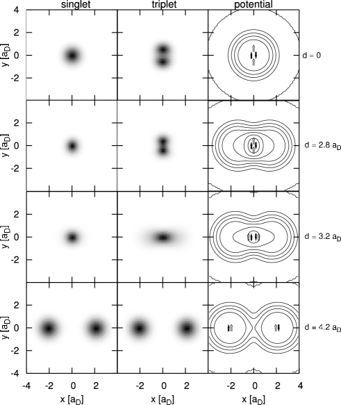
Figure 9: Contours of the one-electron density distribution for the singlet (left panel) and triplet (middle panel) states, and the corresponding confinement potential profiles (right panel) for different distances $d$ between the potential well centres in the case of the hard confinement potential with $p=4$ and $R=2a_{D}$. Full (empty) arrows in the right panel show the sites with the maximum electron density for the singlet (triplet) states.

These effects are additionally illustrated in Figure 9, which displays the contour plots of the one electron density distribution and confinement potential on the $x-y$ plane. The arrows schematically show the sites with the largest electron density for the singlet and triplet states. The plots for $d=0$ and $d=2.8a_{D}$ show that – in the triplet state – each electron is localized at a different site. The plots for $d=2.8a_{D}$ correspond to the maximum of the exchange energy for $p=4$. The triplet electron density distribution is anisotropic on the $x-y$ plane. For small $d$ the electrons with the same spin are aligned in the $y$ direction. This configuration rapidly changes for $d\simeq 3a_{D}$ and the triplet density distribution becomes more spread out in the $x$ direction (cf. Figure 9 for $d=3.2a_{D}$). Figures 7, 8, and 9 show that – for large interdot distances – the electron density distribution is the same in the singlet and triplet which leads to the singlet-triplet degeneracy, i.e., the exchange energy tends to zero for large $d$.

Figure 10 displays the dependence of maximum exchange energy $E_{X}^{max}$ (cf. Figure 6) on parameter $p$ and range $R$ of the confinement potential. The maximum exchange energy increases with increasing parameter $p$, i.e., increasing hardness of the confinement potential, and is the largest for the rectangular-like potential well. However, the maximum triplet-singlet splitting quickly decreases with increasing range $R$, i.e., increasing QD size. The $R$-dependence of $E_{X}^{max}$ allows us to determine the size effect in the exchange interaction [11]. This dependence can be parametrized as follows:

$$E_{X}^{max}(R)=a/R+b\;,$$

with $a=9.975$ and $b=-0.073$ (in donor units).

Figure 10: Maximum exchange energy $E_{X}^{max}$ as a function of range $R$ of the confinement potential (solid curve for $p=4$) and softness parameter $p$ (dashed curve for $R=2a_{D}$) calculated for $V_{0}=25\;R_{D}$.

For fixed parameters $p$ and $V_{0}$ the maximum exchange energy depends not only on $R$, but also on distance $d$ between the centres of the confinement potential. Therefore, the intercentre distance $d=d^{max}$, which corresponds to the maximum of the exchange energy, changes along the curves $E_{X}^{max}(R)$ and $E_{X}^{max}(p)$ in Figure 10. The dependence of $d^{max}$ on parameters $R$ and $p$ is plotted in Figure 11. It appears that intercentre distance $d^{max}$ is a linear function of confinement potential range $R$. Figures 10 and 11 allow us to determine the parameters of the QD nanostructure, for which the exchange energy is maximal. As we have pointed out these parameters correspond to the inner-outer QD nanostructure (cf. Figures 2 and 6). For the coupled QD’s separated by the potential barrier the exchange energy is considerably smaller.

Figure 11: Distance $d^{max}$ between the confinement potential centres, for which the exchange energy is maximal, as a function of confinement potential range $R$ (solid curve for $p=4$) and softness parameter $p$ (dashed curve for $R=2a_{D}$).

4 Discussion

The parametrization of the confinement potential given in Eq. (4) is sufficiently flexible to model various types of QD’s, among them the electrostatically gated QD’s [7] and self-assembled QD’s with the compositional modulation [26]. Using the confinement potential (4) we can describe the effects of smoothness of the QD boundaries [27]. For the intermediate separations $d$ between the potential-well centres ($d\simeq 3a_{D}$ for $R\simeq 2a_{D}$) the resulting potential profile corresponds to the core-shell QD nanostructure with the attractive core potential well. This profile of the confinement potential is characteristic for the compound QD nanostructure with the inner and outer QD’s, which has been recently realized by the chemical growth of self-assembled CdTe/CdS QD’s [28]. The inner-outer QD nanostructure can also be realized in the laterally coupled electrostatically gated QD’s [7]. The corresponding profile of the confinement potential can be obtained by applying the suitably tuned external voltages to the two pairs of different gates. When varying the external voltages, we can tune the shape of the confinement potential, which in turn leads to a desirable change of the exchange interaction.

We have shown that the exchange energy is maximal for the compound QD’s, which consists of the inner QD with the deep potential well and outer QD with the shallow potential well. The maximum of the exchange energy is caused by the strong electron localization in the inner QD and the large difference of the electron localization between the singlet and triplet states (cf. Figures 7, 8, and 9). This result gives us a possibility of designing the nanostructures, in which the exchange interaction is sufficiently large to be used in quantum logic gates [6]. The strong exchange interaction is very important for performing high-fidelity quantum logic operations with spin qubits in QD’s [1, 2, 3, 6]. The recent study [6] of the exchange-interaction induced spin swap operation shows that the swapping the electron spins is very effective, i.e., the electron spins are fully interchanged in the possibly short time, if the confinement potential changes from the double potential wells separated by the barrier to the deep potential well located inside the shallow potential well. The later potential profile corresponds to the inner-outer QD nanostructure [cf. Figure 2(b,c)].

The exchange interaction in the coupled QD’s can also be tuned by applying the external magnetic [16, 17, 20] and electric [8] fields. The increasing magnetic field causes the decrease of the exchange interaction energy since it lowers the energy of the triplet state and leads to the singlet-triplet degeneracy for high magnetic fields [16, 17]. The rapid changes of the external electric field enabled Petta et al. [8] to perform a coherent manipulation of spin qubits in laterally coupled QD’s. Szafran et al. [16] showed that the asymmetry of the QD’s considerably increases the exchange energy. The size effects in the exchange coupling were studied by Zhang et al. [11]. The increasing size of the QD nanostructure leads to the decrease of the exchange interaction due to the decreasing interdot tunnelling [11]. Using the present results we can also determine the size effect in the exchange coupling. In particular, Figure 10 shows that the exchange energy scales as $\sim 1/R$ with the increasing size $R$ of the QD’s.

5 Conclusions and Summary

In the present paper, we have studied the lowest-energy singlet and triplet two-electron states in laterally coupled QD’s and determined the exchange interaction between the electrons. The application of the two-centre PE function parametrization [Eq. (4)] enabled us to investigate a large class of realistic confinement potentials with different shapes. We focus on the dependence of the exchange energy on the distance between the confinement potential centres and also on the shape and range of this potential. The dependence of the exchange energy on intercentre distance $d$ is qualitatively different for the soft ($p=2$) and hard ($p\geq 4$) confinement potentials. For $p=2$ the exchange energy is a monotonically decreasing function of $d$, while for $p\geq 4$ the exchange energy increases with $d$ for small $d$, reaches the maximum for intermediate $d$, and next decreases to zero for large interdot separations. This knowledge allows us to predict the nanostructure parameters, in particular their size and geometry, which maximize the exchange energy.

In summary, we have found that the exchange energy is maximal for the confinement potential, which corresponds to the compound QD nanostructure, consisting of the inner QD with deep potential well embedded in the outer QD with shallow potential well. The corresponding core-shell confinement potential can be obtained in the form of the inner-outer QD nanostructure realized in self-assembled QD’s and electrostatically gated QD’s. We have also investigated the tuning of the exchange interaction by changing the parameters of the coupled QD nanostructure and pointed out the importance of the present study for the quantum logic operations with electron spins.

References

References

- [1] Loss D and DiVincenzo D P 1998 Phys. Rev. A 57 120
- [2] Burkard G, Loss D and DiVincenzo D P 1999 Phys. Rev. B 59 2070
- [3] Burkard G, Seelig G and Loss D 2000 Phys. Rev. B 62 2581
- [4] Hu X and Das Sarma S 2001 Phys. Rev. A 61 062301
- [5] Bellucci D, Montani M, Troiani F, Goldoni G and Molinari E 2004 Phys. Rev. B 69 R201308
- [6] Moskal S, Bednarek S and Adamowski J 2007 Phys. Rev. A 76 032302
- [7] Elzerman J M, Hanson R, Greidanus J S, Willems van Beveren L H, De Franceschi S, Vandersypen L M K, Tarucha S and Kouwenhoven L P 2003 Phys. Rev. B 67 R161308
- [8] Petta J R, Johnson A C, Taylor J M, Laird E A, Yacoby A, Lukin M D, Marcus C M, Hanson M P and Gossard A C 2005 Science 309 2180
- [9] Wang L, Rastelli A, Kiravittaya S, Benyoucef M and Schmidt O G 2006 arXiv:cond-mat/0612701v2
- [10] Fuhrer A, Fasth C and Samuelson 2007 Appl. Phys. Lett. 91 052109
- [11] Zhang L-X, Melnikov V, Agarwal S and Leburton J-P 2007 arXiv:cond-mat/0710.5538v1
- [12] Yannouleas C and Landman U 2001 Eur. Phys. J. D 16 373
- [13] Rontani M, Amaha S, Muraki K, Mahghi F, Molinari E, Tarucha S and Austing D G 2004 Phys. Rev. B 69 085327
- [14] Harju A, Siljamäki S and Nieminen R M 2002 Phys. Rev. Lett. 88 226804
- [15] Reimann S M and Manninen M 2002 Rev. Mod. Phys. 74 1283
- [16] Szafran B , Peeters F M and Bednarek S 2004 Phys. Rev. B 70 205318
- [17] Zhang L-X, Melnikov D V and Leburton J P 2006 Phys. Rev. B 74 205306
- [18] Marlo M, Harju A and Nieminen R M 2003 Phys. Rev. Lett. 91 187401
- [19] Wensauer A., Steffens O, Suhrke M and Rőssler U 2000 Phys. Rev. B 62 2605
- [20] Stopa M and Marcus C M 2006 arXiv:cond-mat/0604008v1
- [21] Pedersen J, Flindt CC, Mortensen N A and Jauho A-P 2007 Phys, Rev. B 76 125323
- [22] Nagaraya S, Leburton J-P and Martin R M 1999 Phys. Rev. B 60 8759
- [23] Adamowski J, Bednarek S and Szafran B 2006 Handbook of Semiconductor Nanostructures and Nanodevices ed. Balandin A A and Wang K L (American Scientific Publishers, CA, USA) 1 389
- [24] Ciurla M, Adamowski J, Szafran B and Bednarek S 2002 Physica E 15 261
- [25] Bednarek S, Szafran B, Lis K and Adamowski J Phys. Rev. B 68 155333 (2003)
- [26] Siverns P D, Malik S, McPherson G, Childs D, Roberts C, Murray R, Joyce B A and Davock H 1998 Phys. Rev. B 58 R10127
- [27] Mlinar V, Schliwa A, Bimberg D and Peeters F M 2007 Phys. Rev. B 75 205308
- [28] de Menezes F D, Brasil Jr. A G, Moreira W L, Barbosa L C, Cesar C L, de C. Fereira R, de Farias P M A and Santos B S 2005 Microelectron. J. 36 989
- [29] Adamowski J, Sobkowicz M, Szafran B and Bednarek S 2000 Phys. Rev. B 62 4234
- [30] Davies K T R, Flocard H, Krieger S and Weiss M S 1980 Nucl. Phys. A 342 111