Imaging the Gamma-Ray sky with SPI aboard INTEGRAL

Abstract

The spectrometer SPI on INTEGRAL allows for the first time simultaneous imaging of diffuse and point-like emission in the hard X-ray and soft gamma-ray regime. To fully exploit the capabilities of the instrument, we implemented the MREM image deconvolution algorithm, initially developed for COMPTEL data analysis, to SPI data analysis. We present the performances of the algorithm by means of simulations and apply it to data accumulated during the first 2 mission years of INTEGRAL. Skymaps are presented for the 1809 keV gamma-ray line, attributed to the radioactive decay of ²⁶Al, and for continuum energy bands, covering the range 20 keV – 3 MeV. The 1809 keV map indicates that emission is clearly detected by SPI from the inner Galactic radian and from the Cygnus region. The continuum maps reveal the transition between a point-source dominated hard X-ray sky to a diffuse emission dominated soft gamma-ray sky. From the skymaps, we extract a Galactic ridge emission spectrum that matches well SPI results obtained by model fitting Bouchet et al. (2005); Strong et al. (2005). By comparing our spectrum with the cumulative flux measured by IBIS from point sources, we find indications for the existence of an unresolved or diffuse emission component above $\sim$100 keV.

1 Introduction

The image deconvolution of gamma-ray data is confronted with several problems that are specific to the domain. First, the data are dominated by a strong instrumental background, generated by the interaction of cosmic-rays with the telescope detectors and the surrounding satellite materials. For SPI, typical signal-to-background ratios are of the order of $\sim$1%. Hence, the deconvolution seeks to explain only a tiny fraction of the registered events, while the bulk of the data have to be explained by a model of the instrumental background characteristics. Second, the information measured by the telescope for each registered photon is only indirectly related to its arrival direction. For SPI, the general data space is 3-dimensional, spanned by the pointing number, the detector identifier, and the measured energy. Analysing the data in a single energy band reduces the date space to two dimensions, which differ however considerably in nature from the image space which is spanned by longitude and latitude. Third, measured count rates are generally very low, leading to non Gaussian distributions for the statistical measurement uncertainties. The consideration of the Poissonian nature of the data is in many cases mandatory to derive meaningful error estimates.

All these particularities explain why imaging the gamma-ray sky with SPI aboard INTEGRAL is difficult, and why classical image reconstruction methods rapidly show their limitations in this domain. Statistical noise easily propagates into the reconstructed sky intensity distributions, leading to artefacts that can severely mislead the observer. One may seek to suppress this statistical noise using regularisation methods, premature stopping of the iterations, and/or image smoothing Strong (2003); Knödlseder et al. (2005); Allain & Roques (2006). These tricks go however in general at the expense of flux suppression and a loss in the angular resolution.

We discuss in this paper the application of an alternative method for image deconvolution of INTEGRAL/SPI data which is based on a multiresolution analysis of the data using wavelets. The method is an implementation of the Multiresolution Expectation Maximisation (MREM) algorithm that has been initially developed to perform image deconvolution of gamma-ray data that where acquired by the COMPTEL telescope aboard the Compton Gamma-Ray Observatory (CGRO) Knödlseder et al. (1999a). The algorithm is implemented as the program spi_obs_mrem (version 3.4.0) and is publicly available at the web site http://www.cesr.fr/$\sim$jurgen/isdc. We will demonstrate that MREM is equally well suited for imaging of point source and diffuse emission, that the algorithm is able to cope with large exposure gradients over the imaged field, and that it allows at the same time reliable estimates of gamma-ray intensities from the resulting images. MREM is a convergent algorithm, and it will be shown that its only sensitive parameter is the wavelet thresholding level which has a well defined scaling, allowing for an objective a priori choice of its value.

2 Deconvolution algorithms

2.1 Richardson-Lucy algorithm

The starting point of MREM is the Richardson-Lucy (RL) algorithm Richardson (1972); Lucy (1974) which is widely used for the deconvolution of astronomical images, and which, in particular, has been also successfully employed for the analysis of gamma-ray data of CGRO Knödlseder et al. (1999a); Milne et al. (2000). Starting from an initial estimate $f_{j}^{0}$ for the image which we usually take as a grey image of negligible intensity, RL iteratively improves this estimate using the relation

$$f_{j}^{k+1}=f_{j}^{k}+\delta_{j}^{k}$$ (1)

with

$$\delta_{j}^{k}=f_{j}^{k}\times\sum_{i=1}^{N}\left(\frac{n_{i}}{e_{i}^{k}}-1\right)R_{ij}$$ (2)

being the image increment of iteration $k$ and

$$e_{i}^{k}=\sum_{j=1}^{M}R_{ij}f_{j}^{k}+b_{i}$$ (3)

being the predicted number of counts in data space bin $i$ after iteration $k$, where

• $i$ is the index of the data space, running from $1$ to $N$,

• $j$ is the index of the image space, running from $1$ to $M$,

• $k$ counts the number of iterations, starting with $0$ for the initial image estimate,

• $f_{j}^{k}$ if the intensity in image pixel $j$ after iteration $k$ (units: ph cm^-2s^-1sr^-1),

• $R_{ij}$ is the instrumental response matrix linking the data space to the image space (units: counts ph^-1 cm² s sr),

• $n_{i}$ is the number of counts measured in data space bin $i$ (units: counts),

• $b_{i}$ is the predicted number of instrumental background counts for data space bin $i$ (units: counts).

Convergence of this algorithm may eventually be very slow, in particular if the instrumental background, $b_{i}$, is the dominating term in Eq. (3). Further, the model of the instrumental background may be presented in a parametrised form, e.g. $b_{i}(\mbox{$\beta_{1},..,\beta_{m}$})$, where the background model parameters $\beta_{1},..,\beta_{m}$ are to be determined along with the image deconvolution process.

Convergence acceleration and simultaneous background model parameter fitting is achieved by replacing Eq. (1) by

$$f_{j}^{k+1}=f_{j}^{k}+\lambda^{k}\delta_{j}^{k}.$$ (4)

and by optimising the acceleration factor $\lambda^{k}$ together with the background model parameters $\beta_{1},..,\beta_{m}$ by maximising the log-likelihood function

$$L(\mbox{$\lambda^{k}$},\mbox{$\beta_{1},..,\beta_{m}$})=\sum_{i=1}^{N}n_{i}\ln e_{i}^{k+1}-e_{i}^{k+1}-\ln n_{i}!$$ (5)

with

$$e_{i}^{k+1}=\sum_{j=1}^{M}R_{ij}(f_{j}^{k}+\mbox{$\lambda^{k}$}\delta_{j}^{k})+b_{i}(\mbox{$\beta_{1},..,\beta_{m}$}).$$ (6)

To conserve positivity of the image pixels during the acceleration process (a property which is inherent to the standard RL algorithm) we require $\lambda^{k}\delta_{j}^{k}>-f_{j}^{k}$ for all image pixels $j$.

2.2 MREM algorithm

The RL algorithm as implemeted by Eqs. 4, 2, 5, and 6 does not explicitely take into account the correlation of intensities in neighbouring image pixels. In the case of weak signals, individual pixels are therefore poorly constrained by the data and statistical fluctuations easily propagate in the reconstruction and quickly amplify. One approach to limit this noise amplification is the application of a smoothing kernel to the image increments $\delta_{j}^{k}$, i.e. to replace

$$\delta_{j}^{k}\to\sum_{r=1}^{M}\Pi_{jr}\delta_{r}^{k}.$$ (7)

As an example, the 511 keV allsky map presented in Knödlseder et al. (2005) has been obtained by the RL algorithm using a 5^∘$\times$5^∘ boxcar average. Together with premature stopping of the iterations, this resulted in a basically noise free image of the Galactic 511 keV intensity distribution.

The drawback of this approach is (1) the effective limited angular resolution imposed by the smoothing procedure and (2) the arbitrary stopping of the iterations. In the MREM approach, we circumvent these problems by replacing Eq. 7 by the wavelet filtering step

$$\delta_{j}^{k}\to\sum_{s=1}^{M^{\prime}}W^{-1}_{sj}\eta_{s}^{k}c_{s}^{k}$$ (8)

where

$$c_{s}^{k}=\sum_{j=1}^{M}W_{sj}\delta_{j}^{k}$$ (9)

are the wavelet coefficients of the image increment, $W_{sr}$ is a $M^{\prime}\times M$ matrix that present the wavelet transform (and $W^{-1}_{sj}$ the inverse transform), and

$$\eta_{s}^{k}=\left\{\begin{array}[]{r@{\quad:\quad}l}0&c_{s}^{k}<t_{s}^{k}\\ 1&\mbox{else}\end{array}\right.$$ (10)

is a threshold vector for the wavelet coefficients $c_{s}^{k}$. The threshold vector represents the essence of the filtering step in that it zeros all those wavelet coefficients that fall below a given threshold $t_{s}^{k}$. The idea behind this kind of filtering is that significant image structures are represented by large wavelet coefficients while insignificant structures are represented by small coefficients. The wavelet transform operates globally on the image and therefore introduces pixel-to-pixel correlations on all possible scales, and the careful selection of $t_{s}^{k}$ allows us to keep only structures for which significant evidence is present in the data. Once all significant structures have been extracted, the algorithm stops.

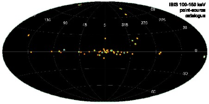
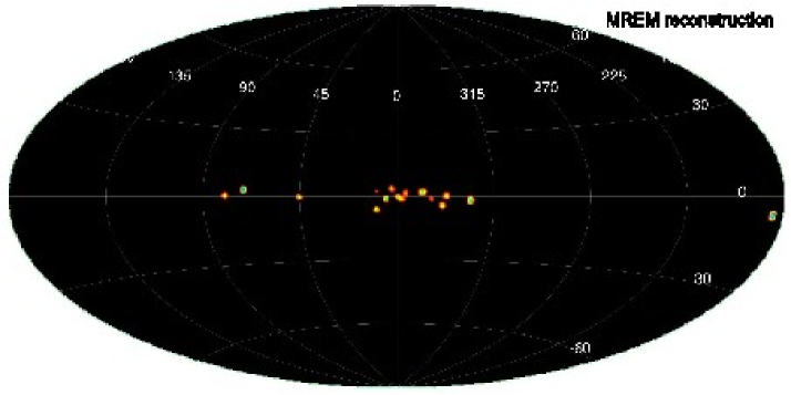
Figure 1: Model (top) and MREM reconstruction (bottom) of a mock dataset of point sources. The simulated sky model is a compilation of IBIS point-sources detected in the 100–150 keV band Bazzano et al. (2006). For the purpose of better visibility, the emission for each source in the model has been spread over a diameter of 2 degrees around the source position. Image reconstruction has been performed using the SPI response in the 100–150 keV energy band.

We estimate $t_{s}^{k}$ for each iteration using Monte-Carlo simulations. For this purpose we create simulated image increments by replacing in Eq. 2 the measured number of counts, $n_{i}$, by the mock data $\tilde{n_{i}}$ which have been drawn from the current estimates $e_{i}^{k}$ using a Poisson random number generator. Since $\tilde{n_{i}}$ are a possible realisation of $e_{i}^{k}$, the resulting image increment reflects now the impact of statistical noise fluctuations only. Transforming this fake image increment in the wavelet domain using Eq. 9 gives then possible values for all wavelet coefficients in the presence of pure statistical noise. Repeating this process a sufficient number of times allows then to estimate the root-mean-square, $\sigma_{s}^{k}$, for each coefficient. We use then these estimates and set the thresholds to

$$t_{s}^{k}=\alpha\times\sigma_{s}^{k}$$ (11)

where $\alpha$ may be interpreted as the number of standard deviations of noise that are allowed during the reconstruction. We found satisfactory results for $\alpha\approx$3.5. 100 Monte Carlo simulations per iteration were found sufficient for reliably estimating the noise levels $\sigma_{s}^{k}$.

3 Simulations

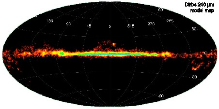
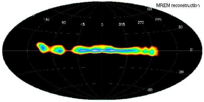
Figure 2: Model (top) and MREM reconstruction (bottom) of a mock dataset of diffuse emission. The simulated sky model is the Dirbe 240 $\mu$m cold dust emission map, scaled to an intensity that corresponds to about 5 times the intensity of the Galactic 1809 keV line emission. Image reconstruction has been performed using the SPI response in a 7 keV wide energy band centred on 1808.5 keV.

To illustrate the performances of MREM we present two simulated reconstructions in Figs. 1 and 2. Both simulations were based on the SPI pointing sequence of the first 2 years of observations, spanning the orbital revolutions 19–269. In both cases, we adopt a realistic model for the instrumental background that was based on the measured data. To simulate the gamma-ray sky, we convolve model intensity distributions with the instrumental response, and add the resulting data space model to that of the instrumental background. Mock data are then generated from these models using our tool spi_obs_sim, which employs a Poisson random number generator to create a realisation of measured events that is statistically compatible with the model.

Our first example illustrates the MREM reconstruction of point source emission (Fig. 1). As sky model we used the IBIS catalogue of 49 sources found in the 100–150 keV energy band Bazzano et al. (2006). The mock dataset has been created and the MREM reconstruction has been performed for the same energy band, but now for the SPI instrument which is less sensitive with respect to IBIS. Consequently, from the 49 simulated sources MREM reaveals only the 15 most brightest ones in the reconstruction. In addition, the modest angular resolution of SPI of $\sim$3^∘ leads to some source confusion towards the densely populated Galactic centre region. Besides the 15 point sources, no other emission features are present, and in particular, the map is free from image noise.

Our second example illustrates the MREM reconstruction of diffuse emission (Fig. 2). As sky model we’ve chosen the Dirbe 240 $\mu$m cold dust emission map which has been shown to provide a reasonable representation of the spatial distribution of 1809 keV gamma-ray line emission attributed to the radioactive decay of ²⁶Al Knödlseder et al. (1999b). In order to highlight details of the reconstruction process, we scaled the intensity of the skymap to approximately 5 times of that expected from 1809 keV line emission. The simulation and reconstruction was performed for a 7 keV wide energy band centred on 1808.5 keV. MREM clearly picks up the basic features of the input map: bright and narrow Galactic ridge emission plus several localised emission features in the Cygnus, Carina and Vela regions. Low-intensity emission that is coded in reddish color in the model map falls apparently below the SPI detection limit, and consequently is clipped by the wavelet filter during the deconvolution. Also for this case, the reconstruction appears to be free of image noise.

Another interesting feature of the MREM reconstruction is the sharpening of the Galactic ridge emission towards the regions of high-intensity in the inner Galaxy. Since the signal in this area is detected at higher statistical significance, the data allow to constrain the intensity profile more precisely, and the reconstructed profile becomes sharper. Further away from the Galactic centre, say beyond $\pm$40^∘ Galactic longitude, the weaker signal intensity makes the data less constraining, and consequently, the reconstructed profile becomes broader. This behaviour is well known in statistics as the bias-variance trade-off, which generally occurs when we try to separate signal from noise using smoothing or correlation techniques.

4 1809 keV gamma-ray line emission

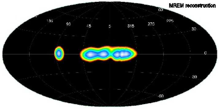
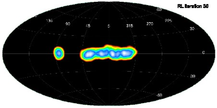
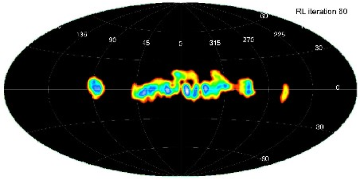
Figure 3: Comparison of MREM (top panel) and RL (middle and bottom panel) reconstructions of 1809 keV data. For RL we show the result after iteration 30 and 60. To reduce the image noise, we applied a boxcar average of 15^∘$\times$15^∘ for the RL reconstruction.

We now apply the MREM algorithm to real data. The dataset we used is the same as that employed for the simulations: the first 2 years of INTEGRAL/SPI observations, spanning the orbital revolutions 19–269. As usually in our analyses, we screened the data for solar flares, exceptionally high countrates, and other possible problems.

Our first goal is to image the sky in the 1809 keV gamma-ray line attributed to the radioactive decay of ²⁶Al. Similar to the simulation, we analyse the data in a 7 keV wide energy band centred on 1808.5 keV. To fully exploit the sensitivity of SPI we use both single and double events. The resulting MREM image is shown in the top panel of Fig. 3. For comparison, we also show the results of the RL reconstruction after iterations 30 and 60 in the middle and bottom panels of Fig. 3. To reduce image noise in the RL reconstruction we applied a boxcar average of 15^∘$\times$15^∘ to smooth the image increment after each iteration (cf. Eq. 7). The images may also be compared to the RL image presented in Diehl (2006) which uses an exponential disk as initial image estimate $f_{j}^{0}$ and for which no boxcar averaging has been performed.

The MREM image indicates that 1809 keV line emission is clearly detected by SPI from the inner Galactic radian (say between $\pm$45^∘ Galactic longitude) and from the Cygnus region (situated in the Galactic plane at $\sim$80^∘ longitude). The inner Galaxy emission shows some local maxima, but those are probably of low statistical significance. Indeed, when we increase the wavelet threshold level from our standard value of $\alpha$=3.5 to 4 most of these maxima disappear, suggesting that the features were probably linked to statistical noise fluctuations.

COMPTEL observations have indicated 1809 keV line emission also from the Carina and Vela regions, located along the Galactic plane at longitudes $\sim$286^∘ and $\sim$266^∘, respectively Knödlseder et al. (1996); Diehl et al. (1995). The RL reconstruction shows indeed a hint for emission from Carina (visible after iteration 60), but the large amount of structure in the image towards the inner Galaxy – which is due to statistical noise fluctuations – indicates that the significance of the Carina feature is weak in our analysed SPI dataset. So far our imaging analysis shows no indication for 1809 keV line emission from the Vela region, but also in the COMPTEL data, the statistical significance of this feature was among the weakest (see also Schanne et al., these proceedings).

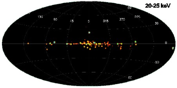
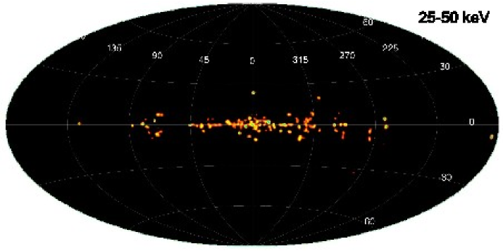
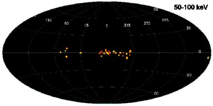
Figure 4: MREM images of the hard X-ray sky in the continuum energy bands 20–25, 25–50, and 50–100 keV.

It is interesting to note that the RL image after iteration 30 appears similar to the MREM image. The heavy boxcar smoothing of 15^∘$\times$15^∘ that we applied during the RL deconvolution plays apparently a similar role as the wavelet filter in that it suppresses high-frequency image noise during the reconstruction. However, the RL iterations do not stop at this point, and even such heavy smoothing does not prevent the growth of image noise in the reconstructions with proceeding iterations. Although we have not formulated an explicit stopping criterion for RL, the algorithm did indeed stop after 85 iterations with an image similiar to that shown after iteration 60. In fact, at this point the image increment smoothing did prevent any further improvement of the likelihood, so the iterations were aborted.

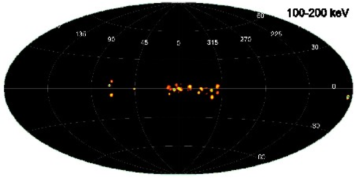
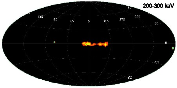
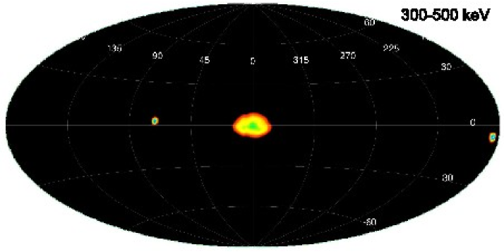
Figure 5: MREM images of the hard X-ray and soft gamma-ray sky in the continuum energy bands 100–200, 200–300, and 300–500 keV.

5 Galactic continuum emission

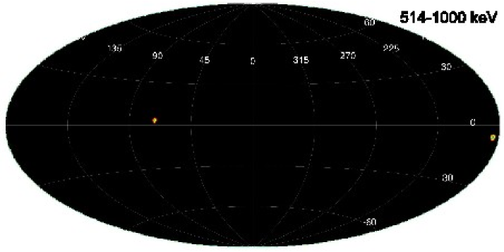
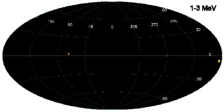
Figure 6: MREM images of the gamma-ray sky in the continuum energy bands 514–1000 keV, and 1–3 MeV.

Our second goal is the imaging of the hard X-ray and soft gamma-ray emission in broad continuum energy bands. This energy range is a transition region where at least three emission components are present: (1) soft ($\mathrel{\mathchoice{\vbox{\offinterlineskip\halign{\hfil$\displaystyle#$\hfil\cr<\cr\sim\cr}}}{\vbox{\offinterlineskip\halign{\hfil$\textstyle#$\hfil\cr<\cr\sim\cr}}}{\vbox{\offinterlineskip\halign{\hfil$\scriptstyle#$\hfil\cr<\cr\sim\cr}}}{\vbox{\offinterlineskip\halign{\hfil$\scriptscriptstyle#$\hfil\cr<\cr\sim\cr}}}}$300 keV) point source emission from Galactic X-ray binaries and AGNs, (2) diffuse bulge dominated emission up to 511 keV attributed to ortho-positronium annihilation, and (3) hard ($\mathrel{\mathchoice{\vbox{\offinterlineskip\halign{\hfil$\displaystyle#$\hfil\cr>\cr\sim\cr}}}{\vbox{\offinterlineskip\halign{\hfil$\textstyle#$\hfil\cr>\cr\sim\cr}}}{\vbox{\offinterlineskip\halign{\hfil$\scriptstyle#$\hfil\cr>\cr\sim\cr}}}{\vbox{\offinterlineskip\halign{\hfil$\scriptscriptstyle#$\hfil\cr>\cr\sim\cr}}}}$300 keV) extended Galactic plane emission of yet unknown nature, possibly linked to the interaction of cosmic-rays with the interstellar medium. The spectral characteristics of these 3 components have been already extensively studied with SPI Bouchet et al. (2005); Strong et al. (2005), but images of this transition region, in particular above $\mathrel{\mathchoice{\vbox{\offinterlineskip\halign{\hfil$\displaystyle#$\hfil\cr>\cr\sim\cr}}}{\vbox{\offinterlineskip\halign{\hfil$\textstyle#$\hfil\cr>\cr\sim\cr}}}{\vbox{\offinterlineskip\halign{\hfil$\scriptstyle#$\hfil\cr>\cr\sim\cr}}}{\vbox{\offinterlineskip\halign{\hfil$\scriptscriptstyle#$\hfil\cr>\cr\sim\cr}}}}$100 keV have so far only been published for the ortho-positronium annihilation component Weidenspointner et al. (2006).

In Figs. 4–6 we present the MREM reconstructions for 8 energy bands situated between 20 keV and 3 MeV. The hard X-ray images below 100 keV nicely show the population of Galactic point sources, mainly X-ray binaries, of which we detect $\sim$60 in the images below 50 keV and $\sim$25 in the 50–100 keV image. No diffuse emission is visible in the reconstructions, indicating that, if present, such emission should be at a rather low intensity level. In the 100–200 keV image we still count $\sim$18 point sources in the image, without a clear hint for diffuse emission. In the 200–300 keV image, a diffuse and structured emission band along the Galactic plane replaces the region where the point sources were located at lower energies. Emission maxima coincide well with the positions of point sources found in the 100–200 keV image, and we therefore suggest that at least part of the 200–300 keV emission originates from faint and unresolved point sources. We cannot exclude, however, that a substantial fraction of the emission in this energy band is indeed of diffuse nature.

The morphology of the emission changes drastically above 300 keV. The 300–500 keV image is dominated by Galactic bulge emission, which is very similar in morphology to the emission that is observed in the 511 keV gamma-ray line (see Weidenspointner et al., these proceedings). The only point sources that are still clearly present at these energies are the Crab (near the anticentre) and the X-ray binary Cyg X-1. The bulge emission seems to show some flattening which may be taken as an indication of another, yet weaker, underlying emission component that follows the Galactic plane.

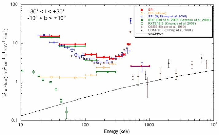
Figure 7: Comparison of the MREM inner Galactic radian spectrum (filled dots) to SPI model fitting results (crosses, Strong et al. (2005)) and to spectra obtained by other instruments. The filled squares show the summed point source contributions from the second IBIS catalogue Bird et al. (2006); Bazzano et al. (2006), normalised to the same Crab spectrum as used for the SPI data. The open dots show the residual MREM flux after subtraction of the IBIS point source contribution. The open squares show the diffuse hard X-ray emission found by Krivonos et al. (2006) using IBIS/ISGRI as a light-bucket. The triangles show the result obtained from COMPTEL data Strong et al. (1994), the diamonds show the OSSE results Kinzer et al. (1999). The black line is the most recent GALPROP model prediction for galactic diffuse emission (Strong, private communication).

Above 514 keV (i.e. at energies situated above the 511 keV positron-electron annihilation line), the gamma-ray sky becomes rather dark (cf. Fig. 6). Only 2 point sources are visible in the 514–1000 keV and 1–3 MeV images, the Crab and Cyg X-1, while no emission can be seen from the Galactic plane. If we would plot the images to very low intensities we would start to see some irregular emission correlated with the Galactic disk, but MREM did not manage to extract this component clearly from the data. In other words, the extended Galactic disk emission that we know from spectral analysis to be present above 514 keV in our SPI observations Bouchet et al. (2005); Strong et al. (2005) is too weak to be reliably imaged with the present dataset.

However, we can determine the global intensity of the Galaxy at these energies by integrating the flux that is present in the MREM images over large regions. We show the result of such an integration in Fig. 7. In order to determine the global flux from the inner Galactic radian, we have chosen an integration region of $\pm$30^∘ in Galactic longitudes and $\pm$10^∘ in Galactic latitudes. We normalised the spectrum to that of the Crab by assuming for the latter a broken power law with a break energy of 117 keV, power law indices of -2.04 and -2.37 for below and above the break, respectively, and a normalisation of 10.78 at 1 keV. We derived this prescription by fitting SPI data of the Crab over the 25–500 keV energy band.

For comparison we show in Fig. 7 also the spectrum that we obtained from SPI data using a model fitting procedure Strong et al. (2005), normalised to the above mentioned Crab spectrum. The MREM result matches quite nicely the spectrum obtained by model fitting. The advantage over the model fitting approach is that the MREM results are unbiased towards assumptions about the spatial distribution of the emission, and this difference may eventually explain the slightly higher fluxes obtained by MREM in the $\sim 100-200$ keV range. The disadvantage is that MREM does not provide an estimate of the statistical uncertainties related to the flux measurements. Hence, both methods are best used in conjunction, providing thus reliable estimates of both the spatial and spectral distribution of the emission.

We also show in Fig. 7 the spectrum that is obtained by summing the flux of all point sources listed in the second IBIS catalogues Bird et al. (2006); Bazzano et al. (2006) within the integration region. We again use the Crab normalisation as for the MREM points to convert the catalogue fluxes (quoted in mCrab) into physical units. For energies below 100 keV, the MREM fluxes match fairly well the point source fluxes determined with IBIS/ISGRI, indicating that most of the emisison in this band can indeed be attributed to point sources Lebrun et al. (2004). Subtracting the IBIS/ISGRI point source flux from the SPI MREM measurements provides an estimate of the unresolved (or diffuse) emission component, which is shown as open dots in Fig. 7. Below $\sim 40$ keV, this estimate is consistent with the findings of Krivonos et al. (2006) who report the detection of an unresolved emission component using IBIS/ISGRI that they attribute to a large population of weak CVs (open squares). Above $\sim 40$ keV, our measurements indicate an additional component that is not resolved by IBIS/ISGRI into point sources. While above $\sim 300$ keV ortho-positronium annihilation towards the galactic bulge may explain partly this discrepancy, the excess emission between $\sim 40-300$ keV can only be attributed to an additional unresolved or diffuse emission component.

We also show in Fig. 7 spectral points obtained by the COMPTEL Strong et al. (1994) and OSSE Kinzer et al. (1999) telescopes, but we did not attempt a cross-calibration using the Crab for these instruments, which may partially explain some apparent discrepancies (even between both instruments). Above 511 keV, the galactic emission is believed to originate mainly from cosmic-rays interacting with the interstellar medium and the interstellar radiation field, and we show in Fig. 7 the latest prediction of the GALPROP cosmic-ray propagation model as solid line (Strong, private communication). Apparently, GALPROP explains relatively well the spectral shape of the unresolved (or diffuse) emission component, both below and above the $511$ keV annihilation line, yet the flux level is underestimated by a factor $\sim 2-3$. Whether this underestimation is due to a yet unrecognised diffuse emission mechanism or due to a yet unresolved weak source population remains to be seen.

Fig. 7 illustrates that MREM images may be exploited quantitatively to derive source spectra. However, such an analysis can not replace a detailed model fitting approach which allows to assess the significance of emission components and to determine the statistical uncertainties in the flux estimates. MREM spectra should therefore be understood as complementary to the model fitting approach in that they do not assume a specific spatial distribution for the emission components. MREM images should hint towards the components that are needed to satisfactorily describe the data, model fitting should then be used to assess how significant these components indeed are.

6 Conclusions

The MREM image reconstruction algorithm presents an interesting alternative for the deconvolution of SPI hard X-ray and gamma-ray data. The main features of this method are (1) the suppression of image noise in the reconstructions and (2) the convergence towards a well-defined solution. The application of MREM to simulations nicely illustrates that these properties are indeed reached by the present implementation.

We employed the algorithm to present SPI images in the 1809 keV gamma-ray line from ²⁶Al and in continuum bands covering energies from 20 keV up to 3 MeV. The 1809 keV image confirms the basic emission features that have been established by COMPTEL, namely the strong Galactic ridge emission from the inner Galaxy, and a prominent emission feature in Cygnus. The continuum images reveal nicely the transition from a point source dominated hard X-ray sky to a diffuse emission dominated soft gamma-ray sky. Imaging the sky above 511 keV is still a challenge, even for MREM, due to the low intensity of the Galactic emission and the correspondingly small signal that is present in the data. Nevertheless, MREM allowed to derive spectral points for the Galactic emission up to 1 MeV, which are in fairly good agreement with previous measurements by OSSE and COMPTEL.

The accumulation of data beyond the 2 years database used for this analysis will enable more detailed imaging of hard X-ray and soft gamma-ray emission throughout the spectrum that is accessible to SPI. We expect to image the diffuse Galactic emission that is underlying the strong ortho-positronium continuum in the intermediate 300–511 keV band, and we hope to visualise also the spatial distribution of Galactic continuum emission above 511 keV. Imaging those emissions will be crucial for the determination of their origin, which theoretically, is still poorly understood Strong et al. (2005).

References

- Allain & Roques (2006) Allain, M. & Roques, J.-P. 2006, A&A, 447, 1175
- Bazzano et al. (2006) Bazzano, A., Stephen, J.B., Fiocchi, M., et al. 2006, ApJ, 649, 9
- Bird et al. (2006) Bird, A.J., Barlow, E.J., Bassani, L., et al. 2006, ApJ, 636, 765
- Bouchet et al. (2005) Bouchet, L., Roques, J.-P., Mandrou, P., et al. 2005, ApJ, 635, 1103
- Diehl et al. (1995) Diehl, R., Bennett, K., Bloemen, H., et al. 1995, A&A, 298, 25
- Diehl (2006) Diehl, R. 2006, in Proc. Nuclei in the Cosmos – IX, astro-ph/0609429
- Kinzer et al. (1999) Kinzer, R.L., Purcell, W.R., and Kurfess, J.D. 1999, ApJ, 515, 215
- Knödlseder et al. (1996) Knödlseder, J., Bennett, K., Bloemen, H., et al. 1996, A&AS, 120C, 327
- Knödlseder et al. (1999a) Knödlseder, J., Dixon, D., Bennett, K., et al. 1999a, A&A, 345, 813
- Knödlseder et al. (1999b) Knödlseder, J., Bennett, K., Bloemen, H., et al. 1999b, A&A, 344, 68
- Knödlseder et al. (2005) Knödlseder, J., Jean, P., Lonjou, V., et al. 2005, A&A, 441, 513
- Krivonos et al. (2006) Krivonos, R., Revnivtsev, M., Churazov, E., et al. 2006, A&A, in press (astro-ph/0605420)
- Lebrun et al. (2004) Lebrun, F., Terrier, R., Bazzano, A., et al. 2004, Nature, 428, 293
- Lucy (1974) Lucy, L. B. 1974, AJ, 79, 745
- Milne et al. (2000) Milne, P. A., Kurfess, J. D., Kinzer, R. L., Leising, M. D., & Dixon, D. D. 2000, AIP Conference Proceedings, 510, 21
- Richardson (1972) Richardson, W. H. 1972, J. Opt. Soc. Am., 62, 55
- Strong et al. (1994) Strong, A.W., Bennett, K., Bloemen, H., et al. 1994, A&A, 292, 82
- Strong (2003) Strong, A.W. 2003, A&A, 411, 127
- Strong et al. (2005) Strong, A.W., Diehl, R., Halloin, H., et al. 2005, A&A, 444, 495
- Weidenspointner et al. (2006) Weidenspointner, G., Shrader, C.R., Knödlseder, J., et al. 2006, A&A, 450, 1013