Causal Set Topology

Abstract

The Causal Set Theory (CST) approach to quantum gravity is motivated by the observation that, associated with any causal spacetime $(M,g)$ is a poset $(M,\prec)$, with the order relation $\prec$ corresponding to the spacetime causal relation. Spacetime in CST is assumed to have a fundamental atomicity or discreteness, and is replaced by a locally finite poset, the causal set. In order to obtain a well defined continuum approximation, the causal set must possess the requisite intrinsic topological and geometric properties that characterise a continuum spacetime in the large. The continuum approximation thus sets the stage for the study of topology in CST. We review the status of causal set topology and present some new results relating poset and spacetime topologies. The hope is that in the process, some of the ideas and questions arising from CST will be made accessible to the larger community of computer scientists and mathematicians working on posets.

1 The Spacetime Poset and Causal Sets

In Einstein’s theory of gravity, space and time are merged into a single entity represented by a pseudo-Riemannian or Lorentzian geometry $g$ of signature $-+++$ on a differentiable four dimensional manifold $M$. Unlike a Riemannian space in which the distance between two distinct points is always positive definite, a Lorentzian geometry is characterised by the fact that this distance can be positive definite (spacelike), negative definite (timelike) or zero (null).

The classical theory of gravity is determined by the Einstein field equations, a non-linear set of second order partial differential equations which relate the spacetime geometry $g$ to classical non-gravitational or matter fields . Geometries which obey the Einstein field equations include simple ones like flat, or Minkowski spacetime, as well as exotic ones containing blackholes. To date, the theory is observationally sound, being consistent with observations spanning lengths scales from the orbits of geocentric satellites to the expansion of the observable universe. At smaller length scales, including human scales and all the way down to nuclear scales, the effects of spacetime curvature are deemed negligible, which means that Einstein gravity can be functionally replaced by Newtonian gravity.

Despite this satisfactory performance however, the theory is not without serious theoretical flaws. Spacetimes which satisfy Einstein s equations can contain “singular” points at which the geometry is ill-defined or the associated curvature diverges, an example being the initial “big-bang” singularity of an expanding universe. The structure of a classical spacetime no longer sustains near such a point and hence the classical geometry is inadequate to answer the question – what is the nature of the singularity? Moreover, at atomic and nuclear scales, the matter fields themselves become quantum in character, and one has to replace Einstein’s equations with an ill-understood hybrid in which classical spacetime interacts with quantum matter. Results from the hybrid theory challenge several cherished notions in physics, a prime example being the so-called “information loss paradox” in the presence of blackholes [2]. They suggest the existence of an underlying, fully quantum theory of gravity in which spacetime itself is “quantised”.

What the nature of such a fundamental theory should be is anybody’s guess, since there are almost no observational constraints on the theory except those coming from its limits to both non-gravitational quantum theory ($G\rightarrow 0$) and Einstein gravity ($\hbar\rightarrow 0$). The different approaches to quantum gravity adopt different cocktails of physical principles and include string theory, loop quantum gravity, spin foams, dynamical triangulations, causal set theory and others. However, a universal characteristic of any such theory which mixes quantum (characterised by the Planck constant $\hbar=10^{-34}J.s$) with gravity (characterised by the gravitational constant $G=6.67\times 10^{-11}m^{3}/kg/s^{2}$ and the speed of light in vacuum $c=3\times 10^{8}m/s$), is the existence of a fundamental length scale, the Planck scale $\ell_{p}=\sqrt{G\hbar c^{-3}}\sim 10^{-35}m$, 20 orders of magnitude smaller than the nuclear scale.

The interest of the present work lies in the poset based approach of causal set theory (CST) [3]. The physical principles that guide this approach are causality, local Lorentz invariance and the assumption of a fundamental spacetime atomicity. CST posits that the underlying structure of spacetime is a locally finite partially ordered set, the causal set with the order relation corresponding to the so-called causal relation in the continuum approximation.

To motivate this approach, let us look more closely at the properties of a Lorentzian spacetime $(M,g)$. Because of the signature $-+++$, the set of future timelike directions at any $p\in M$ forms a future light cone in the tangent space $T_{p}M$, with $p$ at its apex, and similarly the set of past timelike directions, a past light cone, as in Fig 1.

Figure 1: The past and future lightcones in the tangent space $T_{p}M$ at a point $p$ in a spacetime $(M,g)$.

The boundary of these lightcones are the future and past null directions. For a $C^{1}$ curve $\gamma$ on $M$, if the tangent vector $\xi(p)$ at every $p\in\gamma$ is always either spacelike, timelike or null, then $\gamma$ is defined to be a timelike, spacelike or null curve, respectively. $\gamma$ is said to be causal if its tangent is everywhere either timelike or null. Causal curves represent pathways for physical signals, i.e., those that travel at or slower than the speed of light. Causal curves on $M$ give rise to a causal order $\prec$ on $M$: For $x,y\in M$, $x\prec y$ if there is a future directed causal curve from $x$ to $y$. Moreover, in any spacetime, every point has a neighbourhood $U\subset M$ such that $(U,\prec_{U})$ is a partial order, where $\prec_{U}$ is determined by causal curves that lie in $U$.

While the causal order is always transitive, it need not be acyclic. Spacetimes can contain so-called “closed causal curves”, favoured by science fiction writers to build time-machines. Indeed, Einstein theory admits such acausal solutions, an example being the Gödel universe [18]. Spacetimes for which the causal order is acyclic are said to be causal, which makes $(M,\prec)$ a partial order. For strongly causal spacetimes, it was shown by Malament [1] that the poset $(M,\prec)$ determines the conformal class of $(M,g)$ with the only remaining freedom given by the local volume element. This can be summarised by the statement “Causal structure+ Volume = Spacetime”.

The CST approach to quantisation gives prime importance to this poset structure of a causal spacetime in the spirit of the Malament result. The assumption of a fundamental spacetime atomicity or discreteness in CST means that not all of $(M,\prec)$ is considered relevant to the underlying quantum theory but only a subset thereof. Such a subset should have the property that regions of finite spacetime volume contain a finite number of elements of the underlying causal set. Discreteness is posited as a cure for the divergences of Einstein’s theory and quantum field theories, and is supported by the existence of a fundamental Planck volume $V_{p}$ suggesting that structures substantially smaller than $V_{p}$ should not be relevant to the theory. The continuum emerges in the large as an approximation, in a manner similar to a continuous stream of water approximating the underlying discreteness of water molecules. This analogy is useful for picturing the continuum approximation, which will be defined more rigourously later in this section. Discreteness is encoded in CST by the assumption of local finiteness, i.e., that the intervals $<x,y>=\{z\in P|x\preceq z\preceq y\}$ have finite cardinality. $(M,\prec)$ is therefore not itself a causal set but contains as a subposet a causal set which approximates to $(M,g)$. Thus, a CST version of Malament’s result reads “Order + Cardinality $\approx$ Spacetime”. This correlation between the spacetime volume and causal set cardinality in the continuum approximation is a key feature of CST.

As an aside, we note that the idea of causality and local finiteness are also natural to a poset model of computation. Computations can be modelled within a non-relativistic framework, with signals assumed to travel at infinite speed, and with an absolute notion of simultaneity. Causality then reduces to a simple arrow of time. However, since signal velocity is physically constrained, there is indeed a “signal velocity cone” similar to the light cone in a spacetime which, roughly speaking, separates events which can influence each other and those that cannot. Any associated distance function will then have a Lorentzian character. Local finiteness, on the other hand, comes from the physical constraint on the number of computations per interval of time. Thus, in a very general sense, a model of computation based on causality and local finiteness is, at the least, a kinematical realisation of a causal set.

As noted above, $(M,\prec)$ is not itself a causal set, which means that $(M,g)$ needs to be discretised to obtain the underlying causal set $C$, keeping in mind the number to volume correspondence. The simplest possible discretisation of a Riemannian space is one that is regular, with a fixed number of lattice points per unit volume. An example of this is the square lattice on the 2 dimensional Euclidean plane. However, regularity is a deceptive concept in the discretisation of a Lorentzian spacetime. Take for example 2-dimensional Minkowski spacetime with the metric $ds^{2}=-c^{2}dt^{2}+dx^{2}$, where $(t,x)$ are the time and space coordinates, and $c$ is the speed of light. A diamond lattice with equally spaced lattice points along constant $u=ct-x$ and $v=ct+x$ null directions appears regular in the $(t,x)$ coordinate system, with an apparently fixed volume to number correspondence, as in Fig 2. Here, the order relation on the lattice is the induced causal order.

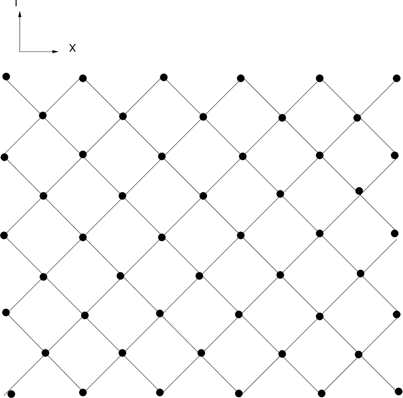
Figure 2: Diamond lattice in a preferred coordinate system

Figure 3: Diamond lattice under a boost.

However, the lattice is no longer regular when acted upon by a “boost” transformation of the coordinates, $B:(t,x)\rightarrow(t^{\prime},x^{\prime})$, the Lorentzian analog of a rotation in Euclidean space. Here, $t^{\prime}=\gamma(t-vx/c^{2})$, $x^{\prime}=\gamma(x-vt)$, where $\gamma={\sqrt{1-v^{2}/c^{2}}}^{-1}$ and $v<c$ is the relative speed between the two coordinate systems. In Euclidean space, a rotation about the origin takes a point $(x_{1},y_{1})$ to another point $(x_{2},y_{2})$ on the constant $r=\sqrt{x_{1}^{2}+y_{1}^{2}}=\sqrt{x_{2}^{2}+y_{2}^{2}}$ circle centred at the origin. Similarly, a boost takes $(t_{1},x_{1})$ to another point $(t_{2},x_{2})$ on the constant $\rho^{2}=c^{2}t_{1}^{2}-x_{1}^{2}=c^{2}t_{2}^{2}-x_{2}^{2}$ hyperbola. Thus, under a boost, the diamond lattice transforms to one in which the lattice points are squeezed together in one null direction and pulled apart in an orthogonal null direction as shown in Fig 3. A large boost with $|v/c|$ close to 1 gives rise to large spacetime “voids”, which violate the number to volume correspondence. In contrast, large voids cannot result from a rotation of a regular lattice in Euclidean space.

How important is invariance under a boost or, Lorentz invariance (LI)? Several approaches to discretisation allow for Lorentz violation [5]. However, LI is a cherished fundamental symmetry of nature, and one which has been experimentally tested to a high degree of accuracy [4]. In order to incorporate it into CST without forfeiting the volume-number correspondence, one has to define the discretisation more carefully. Again, the Euclidean analogy is instructive. For a Euclidean lattice, the continuous rotational symmetry group is replaced by a discrete subgroup which picks out preferred directions. Instead, for a random lattice obtained, for example, by randomly sprinkling points on the plane, there are no preferred directions. Similarly, in CST, spacetime is discretised by a Poisson sprinkling of points in $(M,g)$ which then ensures that there are no preferred directions and hence no Lorentz violation [6]. For a Poisson process the probability of sprinkling $n$ points in a spacetime region of volume $V$ is $P_{V}(n)=\frac{1}{n!}\exp^{-V/V_{c}}(V/V_{c})^{n}$, $V_{c}$ being the discretisation scale. Here $<n>=V/V_{c}$, which means that the volume to number correspondence is satisfied, though only in the mean.

Thus, in order to maintain LI and a reasonable semblance of the volume-number correspondence, the continuum approximation of CST must incorporate a random process. We now define this CST continuum approximation. A causal set $C$ is said to be approximated by a spacetime $(M,g)$ if there is an embedding map $\Phi:(C,\prec)\rightarrow(M,g)$ which is faithful: Let $C$ be a finite causal set with cardinality $V/V_{c}$ and $M$ a finite volume $V$ region of a spacetime. Let $V_{0}$ be the volume of sampling intervals in $M$, with $V_{c}<V_{0}<V$. If $I$ denotes a spacetime interval of volume $V_{0}$, the indicator function $F_{n}=\int\chi_{n}(I)dI/\int dI$ is such that $\chi_{n}(I)=1$, or $0$ depending on whether $I$ contains $n$ elements of the embedded causal set $\Phi(C)$ or not, with the integral over all possible $I$’s in $(M,g)$. Then, if $|F_{n}-P_{V_{0}}|<\delta$, $\Phi$ will be said to be a $\delta$-faithful embedding with respect to $V_{0}$. Faithfully embeddable will henceforth be used in this $(\delta,V_{0})$ sense. In order to make the definition compatible with our intuition, we will also require that $V_{c}\ll V_{0}\ll V$ and $0<\delta\ll 1$. For suitable choices of $\delta$ and $V_{0}$, a causal set generated by a Poisson sprinkling into $M$ with density $V_{c}^{-1}$ is faithfully embedded in $M$. A regular spacetime lattice on the other hand, will not faithfully embed for any reasonable choice of $(\delta,V_{0})$.

In CST, one considers the set of all causal sets, not only those that are obtained via a discretisation of a spacetime. However, in order to make a connection with Einstein theory, causal sets that approximate to spacetimes play a special role. If a causal set is indeed the appropriate discretisation of a continuum spacetime and can capture its large scale structure, then large scale spacetime geometry and topology must be encoded in purely order theoretic terms in the causet. Moreover, if the classical limit of CST is Einstein theory, causal set geometry and topology must play a non-trivial role in CST dynamics. This forms the main motivation for the present work.

If CST is to yield meaningful results, it is also important that the continuum approximation be unique, at least at scales larger than the discreteness scale. This is the key conjecture of causal set theory, also known as its “Hauptvermutung”. It states that if $\Phi:(C,\prec)\rightarrow(M,g)$ is a faithful embedding at density $V_{c}^{-1}$, then $(M,g)$ is unique upto isomorphisms at scales above $V_{c}$. Results in the literature support the idea behind the conjecture, [8, 9, 10] and include recent work on the closeness of Lorentzian spaces [11]. A rigorous statement and proof however, would require a better understanding of how causal set topology and geometry relate to that of the approximating spacetime.

We begin the next section with some definitions from Lorentzian geometry and posets, which will serve as a rough dictionary between the two. In [12] it was shown that a globally hyperbolic spacetime is a bicontinuous poset whose interval topology is the manifold topology. We present an alternative proof, based on a different set of assumptions. This suggests that the condition of global hyperbolicity may be replaced by a weaker causality condition. We then show that, for a causal set that approximates to a causal spacetime $(M,g)$, the chronological relation and the way-below relation coincide. In the following section, we review Sorkin’s arguments for a “finitary” topology [14]. Using a theorem due to McCord [15] we show that for a suitable choice of cover, Sorkin’s finitary structure suffices to capture the continuum topology upto weak homotopy equivalence . In the following section we review results on a finitary construction in CST based on inextendible antichains [16]. This construction reproduces the continuum homology for causal sets that approximate to globally hyperbolic spacetimes and gives important supporting evidence for a topological version of the CST Hauptvermutung. We conclude with some of the open questions on causal set topology.

2 Topology from Causal Structure

By a poset $P$ we mean a set with an order relation $\prec$ which is (i) transitive, i.e., $x\prec y$ and $y\prec z\Rightarrow x\prec z$ and (ii) acyclic, i.e., $x\prec y,y\prec x\Rightarrow x=y$, for any $x,y,z\in P$. Acyclicity is also implied by the irreflexive condition $x\nprec x$, a convention used in much of the causal set literature. We will avoid it here, since it makes the map between the causal set and the continuum a little more cumbersome. The past and future sets of an element $x\in P$ are defined as $\mathrm{Past}(x)\!=\!\{y|y\prec x\}$, $\mathrm{Fut}(x)\!=\!\{y|x\prec y\}$. Without the irreflexive condition therefore, $x$ belongs to its own past and future. A causal set is a poset which is also locally finite: (iii) $|\mathrm{Past}(x)\cap\mathrm{Fut}(y)|<\infty$, where $|A|$ denotes the cardinality of the set $A$.

While all differentiable manifolds, being paracompact, admit metrics of positive definite signature, not all admit Lorentzian metrics. We will only concern ourselves here with those that do. As described in the introduction, in a Lorentzian spacetime $(M,g)$, the tangent space $T_{p}M$ at $p\in M$ is divided into timelike, null and spacelike vectors, which, because of the $-+++$ signature form lightcones. We will henceforth assume here that all spacetimes are time-orientable, so that a consistent notion of future and past directed vector fields is possible everywhere on $(M,g)$.

The causal past and future of $x$ are defined as $\mathbf{J}^{-}(x)=\{y|y\prec x\}$, $\mathbf{J}^{+}(x)=\{y|x\prec y\}$, respectively. Note that since a causal vector can have zero norm, $x\prec x$. The poset analog of an interval in $(M,\prec)$ is then the set $\mathbf{J}^{+}(x)\cap\mathbf{J}^{-}(y)$.

The Lorentzian signature means that spacetimes are endowed with another order relation: $x\prec\!\prec y$ if there exists a $C^{1}$ curve from $x$ to $y$ whose tangent is everywhere future timelike. Again, $\prec\!\prec$ is transitive, and for a causal spacetime, also acyclic. However, $\prec\!\prec$ is irreflexive since $x$ cannot link to itself via a curve whose tangent is everywhere strictly of negative norm. The associated chronological past and future of $x$ are defined as $\mathbf{I}^{-}(x)=\{y|y\prec\!\prec x\}$ and $\mathbf{I}^{+}(x)=\{y|x\prec\!\prec y\}$, respectively. In the manifold topology, $\mathbf{I}^{\pm}(x)$ are open sets, while $\mathbf{J}^{\pm}(x)$ is closed only for a limited class of spacetimes. A generalised transitivity condition states that $x\prec\!\prec y\prec z\Rightarrow x\prec\!\prec z$, and $x\prec y\prec\!\prec z\Rightarrow x\prec\!\prec z$.

As pointed out in [12], the chronological relation $\prec\!\prec$ has an analog in posets in the way below relation $\prec\!\prec_{\mathsf{b}}$ and its dual the way above relation $\succ\!\succ_{\mathsf{a}}$. This relation is defined in terms of directed sets, which appear in domain theory [13]. In a directed set $S$ for every pair $s,s^{\prime}\in S\,\,$, there is an $s^{\prime\prime}\in S$ such that $s,s^{\prime}\prec s^{\prime\prime}$. A filtered set is defined dually. Simple spacetime examples of a directed set are $\mathbf{I}^{-}(x)$, which does not contain its supremum $x$, and $\mathbf{J}^{-}(x)$ which does. However, directed sets are more general than such past sets, and can contain disconnected pieces, an example being a pair of past directed non-intersecting time-like curves from $x$. For $x,y\in P$, $x$ is said to be way below $y$ or $x\prec\!\prec_{\mathsf{b}}y$, if for all directed sets $S$ with a supremum $\bigsqcup S$ and $y\prec\bigsqcup S$, $\exists\,\,s\in S$ such that $x\prec s$. The $\prec\!\prec_{\mathsf{b}}$ relation is a subsidiary relation to $\prec$, similar to how the chronological relation is subsidiary to the causal relation.

The Alexandroff interval in a spacetime is defined to be the open set $\mathbf{I}(x,y)\equiv\mathbf{I}^{+}(x)\cap\mathbf{I}^{-}(y)$. The Alexandroff intervals form a basis for the Alexandroff topology, and it is a well established result in Lorentzian geometry that in a strongly causal spacetime, the Alexandroff topology is the same as the manifold topology [17]. The appropriate poset analog to an Alexandroff interval would then appear to be the interval based on the $\prec\!\prec_{\mathsf{b}}$ relation, $\ll x,y\gg=\{z\in P|x\prec\!\prec_{\mathsf{b}}z\prec\!\prec_{\mathsf{b}}y\}$. For bicontinuous posets, these intervals form the basis for the so-called interval topology on the poset.

Indeed, in [12] it was shown that for globally hyperbolic spacetimes $\prec\!\prec$ and $\prec\!\prec_{\mathsf{b}}$ do coincide in $(M,\prec)$ and hence so do the intervals $\ll x,y\gg$ and $\mathbf{I}(x,y)$. Moreover, $(M,\prec)$ is a bicontinuous poset, which means that the interval topology on $(M,\prec)$ coincides with the manifold topology of $(M,g)$. The results of [12] are striking, in that the full manifold topology of a globally hyperbolic spacetime $(M,g)$ is captured in purely order theoretic terms by the poset $(M,\prec)$. This supplements the result of Malament[1] and places the order theoretic motivations for CST on a firmer footing.

It is therefore of interest to know if the results of [12] hold in spacetimes satisfying weaker causality conditions than global hyperbolicity. The following results are an attempt in this direction. While Lemma 1 holds for any causal spacetime, Lemma 2 replaces the global hyperbolicity condition with a topological requirement on directed sets.

Lemma 1

For a causal spacetime, the $\prec\!\prec_{\mathsf{b}}$ relation in $(M,\prec)$ implies the chronological relation in $(M,g)$.

Proof: Let $x\prec\!\prec_{\mathsf{b}}y$. If we take the directed set $S=\mathbf{I}^{-}(y)$, then $\sqcup S=y$, and $\,\,\exists\,\,s\in\mathbf{I}^{-}(y)$ such that $x\preceq s$. But any such $s\prec\!\prec y$ so that $x\prec\!\prec y$ [17]. $\Box$.

This generalises a part of the proof of [12] to all causal spacetimes, not only those that are globally hyperbolic. To prove the converse, a compactness condition on $\overline{\mathbf{I}(x,y)}$ was used in [12] which requires the spacetime to be globally hyperbolic and not just causal. Instead, if we impose on $(M,\prec)$ the topological condition that for all directed sets $S$, every neighbourhood of $\sqcup S$ has non-trivial intersection with $S$, then we can show the following:

Lemma 2

In a causal spacetime $(M,g)$, if for all directed sets $S$ in $(M,\prec)$ every neighbourhood of $\sqcup S$ intersects $S$ non-trivially, then the chronological relation in $(M,g)$ implies the $\prec\!\prec_{\mathsf{b}}$ relation in $(M,\prec)$.

Proof: Let $x\prec\!\prec y$. Let $S$ be a directed set with $y\prec\sqcup S$. Then, by generalised transitivity, $x\prec\!\prec\sqcup S$. Since $\mathbf{I}^{+}(x)$ is open, this means that there exists a neighbourhood $N$ of $\sqcup S$ such that $N\subset\mathbf{I}^{+}(x)$. From the assumptions on directed sets in $(M,\prec)$, $N\cap S\neq\emptyset$ and hence there exists an $s\in S$ such that $x\prec\!\prec s$. Since this is true for all directed sets, $x\prec\!\prec_{\mathsf{b}}y$. $\Box$

Thus, for any spacetime which is causal and satisfies this topological restriction on directed sets specified in Lemma 2, the way below relation is the chronological relation. As argued in [12], if one further imposes the condition of strong causality, the interval topology on $(M,\prec)$ agrees with the manifold topology on $(M,g)$. Whether this condition on the topology of directed sets translates into a causality condition weaker than global hyperbolicity is currently under investigation [25].

The spacetime $(M,g)$ admits other topologies defined via the order relations $\prec$ and $\prec\!\prec$, distinct from the manifold topology. For past complete spacetimes, consider the open sets to be $\mathbf{I}^{+}(x)$. It is easily seen that the associated topology is $T_{0}$: for any $x\prec y$ and every $w\in M$ such that $x\in\mathbf{I}^{+}(w)$, $y\in\mathbf{I}^{+}(w)$, so that every open set containing $x$ also contains points in its chronological future. However, for every $x\prec y$, $\,\,\exists\,\,z\in M$ such that $y\in\mathbf{I}^{+}(z)$, but $x\notin\mathbf{I}^{+}(z)$. Finally, for $x,y$ spacelike to each other, there exist a pair $w\prec\!\prec x$, $z\prec\!\prec y$ such that $x\in\mathbf{I}^{+}(w),y\notin\mathbf{I}^{+}(w)$ and $y\in\mathbf{I}^{+}(z),x\notin\mathbf{I}^{+}(z)$. This topology is therefore not $T_{1}$ and hence insufficient to describe the Hausdorff topology on $M$.

We have so far steered clear of the condition that makes a poset a causal set, namely, local finiteness. We remind the reader that the poset of interest to CST is not $(M,\prec)$ itself, but the causal set $(C,\prec)$ which faithfully embeds into $(M,g)$. $C$ is therefore not continuous, and hence the results of [12] are not immediately applicable to CST. However, local finiteness simplifies some things. In particular, if $\Phi:(C,\prec)\rightarrow(M,g)$ is a faithful embedding, $\prec\!\prec_{\mathsf{b}}$ in $C$ is indeed equivalent to the chronological relation in $\Phi(C)\subset M$, as we now show.

First, we note that for any directed set $S$ with supremum $\sqcup S$ in a locally finite poset $C$, $\sqcup S\in S$ and is therefore a maximal element. The proof is simple. Assume that $\sqcup S\notin S$. Let $s\in S$, so that the interval $<s,\sqcup S)>\neq\emptyset$ and let its cardinality be $a<\infty$ (by local finiteness). Let $s_{1}\in S\cap\mathrm{Fut}(s)$, so that $<s_{1},\sqcup S>$ has cardinality $a_{1}<a$. Next, let $s_{2}\in S\cap\mathrm{Fut}(s_{1})$ such that $<s_{2},\sqcup S>$ has cardinality $a_{2}<a_{1}$ and so on. This gives a finite, exhaustive set $\{s_{1},s_{2}\ldots s_{k}\}$ so that $a_{k}=2$, i.e., $<s_{k},\sqcup S>$ contains only $s_{k}$ and $\sqcup S$. Now, for any $s^{\prime}\in S$, there exists an $s^{\prime\prime}\in S$ such that $s^{\prime\prime}\succ s_{k}$ and $s^{\prime\prime}\succ s^{\prime}$. This means that $s^{\prime\prime}=s_{k}$, or that $s_{k}$ is to the future of all $s^{\prime}\in S$ and hence the supremum of $S$, which is a contradiction.

Lemma 3

For a causal set $C$ that faithfully embeds into a causal spacetime $(M,g)$, the relation $\prec\!\prec_{\mathsf{b}}$ in $C$ is the same as the chronological relation in $\Phi(C)\subset M$.

Proof: Let $x\prec\!\prec_{\mathsf{b}}y$ in $C$. Choose $S=\mathrm{Past}(y)$, so that $\sqcup S=y\in S$. Then there exists an $s\in S$ such that $x\prec s$. Since $s\prec y$ this means that $x\prec y$. For a causal set that embeds into a spacetime it is therefore possible that $y$ lies on the future lightcone of $x$, or that they can only be joined by a future directed null curve. However, for a faithful embedding, given an $x\in M$, the probability for this is zero . Thus, with probability one, $x\prec\!\prec y$. To prove the converse is easier than in the continuum, because of the simplicity of directed sets in $C$. If $x\prec\!\prec y$, and $S$ a directed set with $y\prec\sqcup S$, then since $\sqcup S\in S$, $x\prec\!\prec y\prec\sqcup S$, $\Rightarrow x\prec\!\prec\sqcup S$ and hence $x\prec\sqcup S$, so that $x\prec\!\prec_{\mathsf{b}}y$. $\Box$

Thus, the intervals $\ll x,y\gg$ in $C$ correspond to Alexandroff intervals $\mathbf{I}(x,y)$ in $(M,g)$. However, since not all Alexandroff intervals in $(M,g)$ are generated by $\ll x,y\gg$ in $C$, the interval topology does not have a simple relationship to the manifold topology. Indeed, in the continuum approximation, only “relevant” continuum topology can be obtained from the causal set. One way to do this might be to consider a subcover of the Alexandroff topology which obtains from $C$, and ask how much of the topology of $(M,g)$ it encodes. This question was posed in a more general context by Sorkin in [14], by replacing the continuum by a finitary substitute. This is the topic of the following section.

3 Finitary Topology

The idea of the continuum is based on the assumption that an infinite resolution of the events in a spacetime is possible, at least in principle. Even without considering quantum effects, this assumption begs the question: given the limited resolution of measurement devices how much of a continuum spacetime (assuming it exists) do we actually probe, and what is its relation to the continuum? In [14] it was suggested that the answer to this question may lie in replacing the continuum topology with a subtopology of locally finite(LF) open coverings. This yields a “finitary” substitute for the full topology, which we can use to address the above question.

We now review this construction. Let $\mathcal{O}=\{O_{i}\}$ be an LF cover of $X$, i.e., every $x\in X$ has a neighbourhood $N\ni x$ such that $N\cap O_{i}\neq\emptyset$ for only a finite number of $O_{i}$. This space can be made into a $T_{0}$ space by defining the equivalence $x\sim y$ if $x\in O_{i}\Leftrightarrow y\in O_{i}$ for all $O_{i}\in\mathcal{O}$. The “finitary” quotient space $\mathcal{F}=X/\sim$ carries the induced topology $\mathcal{T}_{\mathcal{F}}$ on $\mathcal{F}$ with the sets $\{f_{1},f_{2}\ldots f_{k}\}\subset\mathcal{F}$ being open if their inverses under the quotient map are open in $\mathcal{O}$. For every $f_{1},f_{2}\in\mathcal{F},f_{1}\neq f_{2}$, there exists an open $U\in\mathcal{T}_{\mathcal{F}}$, such that either $f_{1}\in U,f_{2}\notin U$ or vice versa. Thus, $\mathcal{F}$ can be endowed with a $T_{0}$ topology. The worry of all discretisation procedures is how much relevant continuum information is lost in the process. For example, would $\mathcal{T}_{\mathcal{F}}$ have sufficient information to be able to recreate the topological invariants of $X$?

In [14] it was shown that this $T_{0}$ quotient does contain non-trivial topological information, by defining, further, a partial order $P(\mathcal{F})$ from $\mathcal{T}_{\mathcal{F}}$. The neighbourhood of any $[x]\in\mathcal{F}$ is defined as $\Lambda([x])=\cap\{U\in\mathcal{T}_{\mathcal{F}}|[x]\in U\}$. Then, $[x]\prec[y]$ in $P(\mathcal{F})$ iff $\Lambda([x])\subset\Lambda([y])$. This poset can be endowed with non-trivial topologies. As shown in [14], in certain examples, the chain complex on $P(\mathcal{F})$ is homotopic to $X$, thus suggesting a potential connection between finitary topology and that of $X$. The full topology of a bounded $T_{1}$ space $X$ is recovered by taking a directed collection of finite open covers $\mathcal{O}_{i}$ of $X$, so that the finitary spaces $\mathcal{F}(\mathcal{O}_{i})$ converge to $X$ as the $\mathcal{O}_{i}$ become more refined. In this sense, $X$ is recovered in the limit of infinite refinement.

However, if discreteness is thought to be fundamental, the recovery of what we will call “irrelevant” topology in the limit is not what we are after. Rather, we would wish for the discrete structure to retain all the relevant features of the continuum without having to go to the limit of infinite refinement. Consider for example a space $X$ with topological structure at scales far smaller than the available resolution. These structures are irrelevant to coarser observations. From the point of view of a measurement, $X$ is equivalent to a space $Y$ which has no topological structures at scales of the order of the discreteness scale.

As we will now show, an appropriate initial choice of $\mathcal{O}$ is indeed sufficient and one does not need to invoke the limit of infinite refinement. Let $P(\mathcal{O})$ be a poset obtained from the relation of set inclusion for a point finite open covering $\mathcal{O}$ of $X$. Let $K(\mathcal{O})$ be the associated chain simplicial complex and $|K(\mathcal{O})|$ the underlying polyhedron with the weak topology. We invoke the following theorem due to McCord [15]:

Theorem 1

(McCord) If $\mathcal{O}$ is a point finite basis-like open cover of $X$ by homotopically trivial sets, then there exists a weak homotopy equivalence $f:|K(\mathcal{O})|\rightarrow X$.

Although the poset $P(\mathcal{O})$ differs in general from that obtained from the finitary space $P(\mathcal{F})$, we show that they are indeed equivalent for coverings which are “sparse” enough. This allows us to use McCord’s theorem to establish a weak homotopy equivalence between $P(\mathcal{F})$ and $X$.

Lemma 4

Let $\mathcal{O}$ be a point finite basis-like simple cover of $X$, such that none of the $O_{i}\in\mathcal{O}$ can be expressed as a non-trivial union of members of $\mathcal{O}$. Then, there exists a map $g:P(\mathcal{F})\rightarrow P(\mathcal{O})$ which is an order preserving bijection, with the order relation in $P(\mathcal{F})$ carrying over to the order relation on $P(\mathcal{O})$. Hence, the chain complex $K(\mathcal{F})$ of $P(\mathcal{F})$ is such that there exists a weak homotopy equivalence $f:|K(\mathcal{F})|\rightarrow X$.

Proof: Let $g([x])=\cap_{\mathcal{O}}\{O\in\mathcal{O}|x\in O\}\equiv O(x)$, i.e. $[x]$ is mapped to the smallest open set in $\mathcal{O}$ containing $x$. For any $y\in X$, if $O(y)\neq O(x)\Rightarrow x\nsim y$. Therefore $g$ is 1-1 and we may write $O([x])\equiv O(x)$. Conversely, associated with each $O$, there is a finite sequence of equivalence classes $\{[x_{1}],[x_{2}],\ldots[x_{k}]\}$ such that every $x\in O$ lies in some equivalence class $[x_{i}]$. Let $\{O(x_{1}),\ldots,O(x_{k})\}$ be the associated open sets. Then there exists an $x_{i}\in O$ such that $O(x_{i})=O$. Else, $O=\cup_{i}O(x_{i})$ and does not belong to the collection $\mathcal{O}$. In other words, for every $O\in\mathcal{O}$ is associated a unique $[x]$ in $\mathcal{F}$. Thus, $g$ is a bijection. That it is further, order preserving, comes from the fact that if $[x]\prec[y]$ in $P(\mathcal{F})$, $\Lambda([x])\subset\Lambda([y])$, while in $P(\mathcal{O})$, $O(x)\prec O(y)$ iff $O(x)\subset O(y)$. Now, under the quotient map, $f(O(x))=\Lambda([x])$. This can be seen as follows. $[x]\in U(\in{{\mathsf{T}}}_{\mathcal{F}})\Leftrightarrow x\in f^{-1}(U)$, $O(x)\subseteq f^{-1}(\Lambda([x])$ since otherwise there exists a smaller $O^{\prime}=f^{-1}(U)\cap O(x)\subset O(x)$ which contains $x$. Assume strict inclusion, i.e., $O(x)\subset f^{-1}(\Lambda([x])$. Then $\exists$ a set $\{[z_{1}],[z_{2}]\ldots[z_{k}]\}\in\mathcal{F}$ such that $z_{i}\in f^{-1}(\Lambda[x])\Rightarrow z_{i}\notin O(x)$. Let this set be exhaustive, i.e., there is no other equivalence class $[z]$ such that $z\in f^{-1}(\Lambda[x]),z\notin O(x)$. Thus, if $f(O(x))=\{[x],[y_{1}],\ldots[y_{l}]\}$ where $x,y_{i}\in O(x)$, then $\Lambda[x]=\{[x],[y_{1}],\ldots[y_{l}],[z_{1}]\ldots[z_{k}]\}$. Since $f(O(x))\subset\Lambda(x)$, it contradicts the claim that $\Lambda(x)$ is the smallest open subset of $\mathcal{T}_{\mathcal{F}}$ containing $[x]$. Since the order relation in both posets is defined purely in terms of set inclusion, and every open set in $\mathcal{O}$ is also a neighbourhood of some $x$, this means that $g$ is an order preserving bijection. It then follows from the theorem of McCord that $f:|K(\mathcal{O})|\rightarrow X$ is a weak homotopy equivalence. $\Box$

Thus, a carefully chosen finitary substructure suffices to capture the relevant topological information of a space. Assuming that the space is topologically trivial at scales below some fixed scale, a LF covering of open sets at this scale can capture the coarse continuum topology.

The considerations above are independent of the signature of the overlying geometry. For a Lorentzian geometry $(M,g)$, a natural choice of topology would be that based on the Alexandroff intervals out of which a sparse, simple subcover may be obtained, so that the associated $|K(\mathcal{F})|$ is weakly homotopic to $M$. Note, however, that the order relation for the poset $P(\mathcal{F})$ does not correspond to the causal order. If at all a relationship exists between a causal set and this finitary poset, it should be more subtle.

4 Causal Set Homology

As shown in the previous section, a weak homotopy correspondence exists for a given class of cover and the underlying space. However what needs to be understood is whether CST hands us the right sort of cover in the continuum approximation, which satisfies the required property of LF and sparseness. For the interval topology on $C$, the associated Alexandroff cover on $(M,g)$ is not LF and hence doesn’t lend itself naturally to the finitary analysis of the previous section. The challenge is to isolate appropriate subsets of $C$ which provide a basis for a topology on $C$, which can then be correlated with the continuum topology in the approximation.

In [16] such a candidate class of subsets was proposed and shown to capture the continuum homology when $(M,g)$ is globally hyperbolic. For such spacetimes $M\sim\Sigma\times\mathbb{R}$, where $\Sigma$ represents a spatial hypersurface, so that $\Sigma$ is a deformation retract of $M$. This allows us to shift the focus away from $M$ to $\Sigma$. The causal set analog of $\Sigma$ is an inextendible antichain $A$ which is a maximal set of unordered points in the causal set. On its own, $A$ is only endowed with the trivial topology, and hence does not suffice to capture the topology of $\Sigma$. Consider instead a neighbourhood of $A$ in $C$, the thickened antichain

$${{\mathsf{T}}}_{\mathsf{n}}(A)\equiv\{\,p\,|\,\,|(\mathrm{Past}(p))\cap\mathrm{Fut}(A)|\leq{\mathsf{n}}\},\quad{\mathsf{n}}\in\mathbb{N}.$$ (1)

Here, ${{\mathsf{T}}}_{1}(A)=A$ and as $\mathsf{n}$ increases, one gets to sample more and more of the future of $A$ in $C$. The past $P_{i}$ of a maximal element $m_{i}\in{{\mathsf{T}}}_{n}(A)$ casts a “shadow” $A_{i}\equiv P_{i}\cap A$, on $A$. For $\mathsf{n}$ finite, the collection $\mathcal{P}\equiv\{P_{i}\}$ covers ${{\mathsf{T}}}_{\mathsf{n}}(A)$, where $i\in[1,\ldots,m]$, $m=|\mathsf{M}|$, for $\mathsf{M}$ the set of maximal elements of ${{\mathsf{T}}}_{\mathsf{n}}(A)$. Similarly, the collection $\mathcal{A}\equiv\{A_{i}\}$, $i\in[1,\ldots,m]$ covers $A$.

The covers $\mathcal{P}$ and $\mathcal{A}$ which occur naturally in the causal set are thus candidates for recovering the large scale topology of the spacetime. In particular, $\mathcal{A}$ is a discrete version of an open cover on $\Sigma$. In order to find the continuum analogue of the thickened antichain, $\Sigma$ must be volume “thickened” to a region $M_{\Sigma}^{\mathsf{v}}$. The volume function is $\mathsf{v}(p)\equiv\mathrm{vol}(\mathbf{I}(\Sigma,p)),\,\,p\in\mathbf{I}^{+}(\Sigma)$, where $\mathrm{vol}(X)$ is the spacetime volume of a region $X\subset M$. The level sets $\Sigma_{\mathsf{v}}$ of $\mathsf{v}$ are homeomorphic to $\Sigma$ and provide a foliation of $M$ to the future of $\Sigma$. $M_{\Sigma}^{\mathsf{v}}$ is thus the region sandwiched between $\Sigma$ and $\Sigma_{\mathsf{v}}$. For any $\mathsf{v}>0$, the intersection of $\mathbf{I}^{-}(x)$ with $\Sigma$ for $x\in\Sigma_{\mathsf{v}}$ is open in $\Sigma$. These shadows provide a cover $\mathcal{O}$ of $\Sigma$, from which a LF subcover $\mathcal{O}_{\mathsf{v}}$ can be obtained. Unlike the discrete case, however, an LF subcover $\mathcal{I}_{\mathsf{v}}$ of the past sets $I(x)=\mathbf{I}(\Sigma,x),x\in\Sigma_{\mathsf{v}}$ does not cover $M_{\Sigma}^{\mathsf{v}}$.

One could at this stage construct a finitary topology of $\mathcal{O}_{\mathsf{v}}$ and find the associated simplicial complex. Before we do this, let us first try to guess the discrete-continuum correspondence that we are seeking. While $\mathcal{O}$ covers $\Sigma$ and are analogs of the cover $\mathcal{A}$ of $A$, these are sets of measure zero in the Poisson sprinkling and hence one cannot directly obtain the correspondence between the two. Instead, one must compare the collections of past sets $\mathcal{P}$ and $\mathcal{I}$. In [16] it was shown that these collections are in 1-1 correspondence with their spatial counterparts $\mathcal{A}$ and $\mathcal{O}$, respectively. An LF collection $\mathcal{O}_{f}$ of $\mathcal{O}$ can be obtained via the continuum pasts of the maximal elements of the thickened antichain. In order to use the results of Lemma [4], $\mathcal{O}_{f}$ must be a point finite, sparse and simple cover. The condition of sparseness is not natural to such a cover, however, and hence an alternative construction is required.

In [16] the finitary topology used was the nerve simplicial complex associated with a cover. In the causal set, the nerves $\mathcal{N}_{\mathsf{n}}(\mathcal{P})$ and $\mathcal{N}_{\mathsf{n}}(\mathcal{A})$ were shown to be homotopic to each other and so too their continuum counterparts $\mathcal{N}(\mathcal{I}_{f})$ and $\mathcal{N}(\mathcal{O}_{f})$. For a generic causal set, $\mathcal{N}_{\mathsf{n}}(\mathcal{A})$ provides a “transient” topology on $A$ since it is in general non-homotopic to $\mathcal{N}_{\mathsf{n}^{\prime}}(\mathcal{A})$ for $\mathsf{n}\neq\mathsf{n}^{\prime}$. While the nerve $\mathcal{N}(\mathcal{O}_{\mathsf{v}})$ also varies with $\mathsf{n}$, an important feature of the continuum is that there is a large enough range of $\mathsf{v}$ for which $\mathcal{N}(\mathcal{O}_{\mathsf{v}})$ is homotopically stable.

Since $(\Sigma,h)$ is itself a Riemannian space, with $h$ the spatial metric on $\Sigma$ induced from $g$, every $x\in\Sigma$ has a convexity radius. This is the largest $\mathfrak{r}_{x}$ such that the distance function is convex on the open ball $B(x,\mathfrak{r}_{x})$ and any two points in $B(x,\mathfrak{r}_{x})$ are joined by unique segments lying entirely in it [19]. The infimum of $\mathfrak{r}_{p}$ over $p\in\Sigma$ gives the convexity radius $\mathfrak{r}$ of $\Sigma$. An open set $O$ is said to be convex with respect to $\mathfrak{r}$ if for any $p,q\in O$, the (unique) geodesic between them of arc-length $<\mathfrak{r}$ lies entirely in $O$. A convex cover of $\Sigma$ is an LF cover of open sets which are convex with respect to $\mathfrak{r}$. The following result due to de Rham and Weil [20] then states

Theorem 2

(De Rham-Weil) The nerve of a convex cover of $\Sigma$ is weakly homotopic to $\Sigma$.

Using the machinery of causal analysis, it was shown in [16] that associated to every $\Sigma$ is a convexity volume $\tilde{\mathsf{v}}$ such that for all $0<\mathsf{v}<\tilde{\mathsf{v}}$, the shadows from $\Sigma_{\mathsf{v}}$ are convex. Thus for any LF subcover $\mathcal{O}_{f}\subset\mathcal{O}$, $\mathcal{N}_{\mathsf{v}}(\mathcal{O}_{f})$ is weakly homotopic to $\Sigma$.

The tricky part is to correlate this result to the nerve $\mathcal{N}_{\mathsf{n}}(\mathcal{P})$ or $\mathcal{N}_{\mathsf{n}}(\mathcal{A})$ obtained from the causal set. Because of the nature of the continuum approximation, the correspondence is a probabilistic one. There are, moreover, crucial differences between the continuum and the causal set. Namely, apart from the upper bound $\tilde{\mathsf{v}}$ coming from convexity considerations, one also has a lower bound $\mathsf{v}_{0}$ coming from the discreteness scale. At such scales, the transient causal set topology $\mathcal{N}_{\mathsf{n}}(\mathcal{A})$ need bear no semblance to the continuum. In general, for small $\mathsf{n}$ it will be made up of several disconnected bits. Thus, it is only in an intermediate range that we can expect a correspondence that will be useful in the sense of Theorem [2]. In such a range, and under certain conditions on the compactness scale of the spacetime, $\mathcal{N}_{\mathsf{n}}(\mathcal{A})$ was shown to be, with high probability, an adequate subcomplex of a $\mathcal{N}(\mathcal{U})$ where $\mathcal{U}$ are open covers induced by the chronological pasts of the maximal elements of ${{\mathsf{T}}}_{\mathsf{n}}(A)$.

Thus if $\Phi:C\rightarrow(M,g)$ is a faithful embedding, then for any inextendible antichain $A$ for which the discreteness scale is sufficiently smaller than the supremum of the convexity volumes of the set of $\Sigma\supset A$, there is a range of $\mathsf{n}$ for which the homology is stable and equivalent to the homology of $M$. While the analytical work uses very stringent conditions to obtain high probabilities, numerical simulations [21] with relatively small causal sets already produce striking results. They suggest a criterion for manifoldlikeness based on the existence of a stable homology, sandwiched between fluctuating homology.

It is useful at this point to compare this construction with that of persistent homology [22]. For calculating the persistent homology of a complex $K$, use is made of a filtration of subcomplexes $\{K_{i}\}$ of $K$, $i=0,\ldots n$, ordered by inclusion $K_{i-1}\subset K_{i}$, with $K_{n}=K$. In the filtration, each simplex is preceded by its faces, so that $K$ can be expressed as an ordered set of simplices. One has the induced homomorphism $f_{p}^{i}:H_{p}(K_{i})\rightarrow H_{p}(K_{i+1})$, which then combines to $f_{p}^{ij}:H_{p}(K_{i})\rightarrow H_{p}(K_{j})$, $0\leq i\leq j\leq n$. Persistent homology then refers to the homology which survives the filtration from the $i$th stage to the $j$th stage, $i\leq j$. Computationally, the filtration provides an advantage, since the homology can be incrementally updated. The idea of persistence thus has a resonance with the nerve construction and the stability of the homology.

However, the set of nerve complexes $\{\mathcal{N}(\mathcal{A}_{\mathsf{n}})\}$, $1\leq\mathsf{n}\leq\mathsf{n}_{0}$ do not provide a filtration for $\mathcal{N}(\mathcal{A}_{\mathsf{n}_{0}})$. This is because for each $\mathsf{n}$, the nerve is constructed from shadows of maximal elements, so that the shadows from stage $\mathsf{n}-1$ are not necessarily contained as vertices in $\mathcal{N}(\mathcal{A}_{\mathsf{n}})$ complex. One could rectify this by simply adding all shadows upto stage $n$, so that shadows from all elements in ${{\mathsf{T}}}_{n}(A)$ are included in the new nerve complex $\tilde{\mathcal{N}}(\mathcal{A}_{\mathsf{n}})$ including the elements of $A$ itself. This enlarges the complex significantly but provides the required filtration. While the simplices are not added stage by stage, one could nevertheless extract the persistent homology groups from this construction. However, in a sense, persistence is already intrinsic to the thickened antichain construction, with the ordering provided by the volume or cardinality function. For example, if at stage $\mathsf{n}_{1}$ the zeroth homology $H_{0}=Z^{p},p>1$ and at stage $\mathsf{n}_{2}$ $H_{0}=Z$, then the “spurious” extra components in $\mathcal{N}(\mathcal{A}_{\mathsf{n}_{1}})$ are discarded in $\mathcal{N}(\mathcal{A}_{\mathsf{n}_{2}})$. Using only the pasts of the maximal elements of ${{\mathsf{T}}}_{\mathsf{n}_{2}}(A)$ is thus sufficient to obtain the required stable or persistent homology. While $\mathcal{N}(\mathcal{A}_{\mathsf{n}})$ has fewer vertices than its filtered counterpart $\tilde{\mathcal{N}}(\mathcal{A}_{\mathsf{n}})$ there may be yet unexplored computational advantages in using the persistent homology algorithms. What we can say definitively, however, is that the vertices of a filtration of $\mathcal{N}_{n}(A)$ will not all have faithful continuum counterparts, since for small thickenings, the associated spacetime regions would be of order the discreteness scale.

5 Open Questions

While there has been progress on the question of causal set topology in the context of the CST continuum approximation, there is much that remains to be understood. Perhaps the strongest result on topology that we might hope for is a topological version of the Hauptvermutung: if $\Phi_{1}:C\rightarrow(M_{1},g_{1})$ and $\Phi_{2}:C\rightarrow(M_{2},g_{2})$ are faithful embeddings, then the topological invariants of the associated finitary topologies $\mathcal{F}_{1},\mathcal{F}_{2}$ should be equal, where the $\mathcal{F}_{i}$ on $M_{i}$ obtain from the embeddings $\Phi_{i}$, $i=1,2$. This would mean that the coarse topology of $C$ uniquely determines the topology of $M$ at scales larger than the discreteness scales.

We are clearly not close to a proof of such a conjecture, but it is not all that far from our sights. Consider the homology construction of the previous section. For a $(\delta,V_{0})$ pair of faithful embeddings $\Phi_{1},\Phi_{2}$, the $H_{i}$ should be constructed from coverings using a $\mathsf{v}\sim V_{0}$, so that the associated homologies are equivalent. Even if one restricts to spacetimes which are globally hyperbolic, our current homology construction does not, at least at present, say anything about the existence and ubiquity of the special class of inextendible antichains used therein. If it were possible to identify or characterise these antichains with no reference to the approximating manifold, we would be close to a homological version of the Hauptvermutung.

In order to make such an identification, one may have to invoke geometric structures on the causal set. Simulations suggest that the desired antichains can be identified by the homogeneity of the extrinsic curvature of the spatial slices which contain them. Indeed, the thickening procedure seems to “flow” any antichain to one that is more homogeneous in this sense, thus suggesting genericity. Progress has been made in this direction using a spatial distance on the antichain induced by the thickening [23].

Of course, the question of how spacetime geometry is encoded in a causal set is itself key to CST. In causal sets that faithfully embed into Minkowski spacetime, it was shown in [10] that the length of the longest antichain between two elements is a good measure of their time-like geodesic distance. Generalising this to arbitrary spacetimes, and finding a bound on the fluctuations would be of considerable interest to the CST community. In order to build a causal set dynamics that mimics that of spacetime, a causal set analog of the curvature is required. While there are hints in this direction [24], it is one of the important open questions of CST.

We end with a comment on the basic assumption of local finiteness. As described in the introduction, this is motivated by the idea of a fundamental atomicity underlying spacetime so that a finite spacetime volume contains a finite number of causal set elements. However, local finiteness is a stronger condition. Let us consider the anti-de Sitter spacetime, described in [18]. This spacetime is not globally hyperbolic, but is otherwise well behaved, satisfying stringent causality requirements. An important global feature is that it contains Alexandroff intervals of infinite volume. Thus, although the number to volume correspondence can be maintained by the Poisson sprinkling, the resulting CST-type discretisation does not produce a locally finite poset. While these spacetimes are perhaps not physically realisable, they may play a non-trivial role in the approach to classicality. Should CST relax local finiteness to a weaker condition or must we accept that such spacetimes lose their relevance in CST? A better understanding of causal set geometry would be essential to help answer this question satisfactorily.

6 Acknowledgements

I thank the organisers of the Dagstuhl seminar for this opportunity to explore the links between spacetime causality and the mathematics of posets. In particular, I thank Jimmy Lawson and Prakash Panangaden for discussions related to this work. This work was supported in part by the Royal Society-British Council International Joint Project.

References

- [1] David Malament, J. Math. Phys 18 1399 (1977).
- [2] S.W. Hawking, Commun. Math. Phys. 43 199 (1975).
- [3] L. Bombelli, J. H. Lee, D. Meyer and R. Sorkin, Phys. Rev. Lett. 59, 521 (1987); R. D. Sorkin, School on Quantum Gravity, Valdivia, Chile, 4-14 Jan 2002. Published in Valdivia 2002, “Lectures on quantum gravity” 305-327, arXiv:gr-qc/0309009.
- [4] T. J. Konopka and S. A. Major, New J. Phys. 4, 57 (2002) [arXiv:hep-ph/0201184].
- [5] M. Gaul and C. Rovelli, Lect. Notes Phys. 541, 277 (2000) [arXiv:gr-qc/9910079].
- [6] L. Bombelli, J. Henson and R. D. Sorkin, arXiv:gr-qc/0605006.
- [7] L. Bombelli. Talk at “Causet 2006: A Topical School funded by the European Network on Random Geometry”, Imperial College, London, U.K., September 18-22, 2006.
- [8] L. Bombelli and D. A. Meyer, Phys. Lett. A 141, 226 (1989).
- [9] D.A. Meyer, “The Dimension of Causal Sets”, Ph.D. thesis, MIT (1988).
- [10] G. Brightwell and R. Gregory, Phys. Rev. Lett. 66, 260 (1991).
- [11] L. Bombelli, J. Math. Phys. 41, 6944 (2000) arXiv:gr-qc/0002053; L. Bombelli and J. Noldus, Class. Quant. Grav. 21, 4429 (2004) arXiv:gr-qc/0402049.
- [12] K. Martin and P. Panangaden, Commun. Math. Phys. 267 (2006) 563 [arXiv:gr-qc/0407094].
- [13] B. A. Davey and H. A. Priestly, “Introduction to Lattices and Order”, Cambridge, Cambridge University Press, 2002.
- [14] R. D. Sorkin, Int. J. Theor. Phys. 30, 923 (1991).
- [15] M.C. McCord, Proc. Amer. Math. Soc. 18 705 (1967).
- [16] S. Major, D. Rideout, S. Surya, J. Math. Phys. 48, 032501 (2007).
- [17] Roger Penrose, “Techniques of Differential Topology in Relativity”, AMS Colloquium Publications (SIAM, Philadelphia, 1972).
- [18] Hawking, S.W. and Ellis, G.F.R., “The large scale structure of space-time”, Cambridge: Cambridge University Press, 1973.
- [19] Petersen, P., “Riemannian geometry”, Graduate Texts in Mathematics, New York:Springer-Verlag, 1998.
- [20] A. Weil, Commentarii Mathematici Helvetici 26, 119-145 (1952). Georges De Rham, Annales de l’institut Fourier 2 51-67 (1950).
- [21] S. Major, D. Rideout and S. Surya, Work in progress.
- [22] H. Edelsbrunner, D. Letscher and A. Zomordian, Discrete Comput. Geom. 28 511, (2002).
- [23] J. Henson, S. Major, D. Rideout and S. Surya, Work in progress.
- [24] R. D. Sorkin, “Does locality fail at intermediate length scales?”, in: Danielle Oriti (ed.), Towards Quantum Gravity, Cambridge University Press, 2006. arXiv:gr-qc/0703099; J. Henson, “The causal set approach to quantum gravity”, in: Danielle Oriti (ed.), Towards Quantum Gravity, Cambridge University Press, 2006. arXiv:gr-qc/0601121.
- [25] Panangaden and Surya, in preparation.