Unambiguous comparison of ensembles of quantum states
Abstract
We present a solution of the problem of the optimal unambiguous comparison of two ensembles of unknown quantum states and . We consider two cases: 1) The two unknown states and are arbitrary states of qudits. 2) Alternatively, they are coherent states of a harmonic oscillator. For the case of coherent states we propose a simple experimental realization of the optimal “comparison” machine composed of a finite number of beam-splitters and a single photodetector.
pacs:
03.67.Lx,02.50.GaI Introduction
In the classical world it is relatively easy to compare (quantitatively, or qualitatively) features of physical systems and to conclude with certainty whether the systems possess the same properties, or not. On the other hand, the statistical nature of the quantum theory restricts our ability to provide deterministic conclusions/predictions even in the simplest experimental situations. Therefore comparison of quantum states is totally different compared to classical situation. To be specific, let us consider that we are given two quantum systems of the same physical origin (e.g., two photons) and our task is to conclude whether these two photons have been prepared in the same polarization state. That is, we want to compare the two states and we want to know whether they are identical or not. Given the fact that we have just a single copy of each state the scenario according to which we first measure each state does not work. For that we would need an infinite ensemble of identically prepared systems. The solution to the problem of comparison of quantum states has been proposed by Barnett et al. jex : Within quantum realm we can compare two states, but there is a price to pay. For instance, one cannot conclude with certainty that two systems are in the same pure state or not, except for the case when the set of possible pure states is linearly independent chefles . The unambiguous state comparison as introduced by Barnett et al. is a positive-operator-value-measure (POVM) measurement that has two possible outcomes associated with the two answers: the two states are different, or outcome of the measurement corresponds to an inconclusive answer. Moreover, the existence of the negative answer strongly depends on the particular quantum states in the following sense. To give the unambiguous conclusion that the states are different it is necessary to restrict ourselves to states, which have distinct supports kleinman . In the quantum comparison problem as discussed by Barnett, Chefles, Jex and Andersson jex ; andersson ; chefles it is assumed that the unknown states are pure and only a single copy of each of them is available.
The aim of the present paper is to find the optimal unambiguous state comparison procedure in the case we have more copies of the two quantum states which we want to compare. Throughout the paper we assume that the compared states are pure and that they belong to a -dimensional Hilbert space . The dimensionality of the Hilbert space in known, otherwise no further information about the states is available. In the case of (semi)-infinite dimensional Hilbert space (corresponding to a harmonic oscillator) we restrict our investigation to a specific case, when we a priori know that the two states to be compared are coherent states. What is not known are their complex amplitudes. Our goal will be to design an optimal quantum comparison machine.
As in the case of only one copy per each of the two compared states it is not possible to unambiguously conclude that the compared states are the same. Thus, the positive operator-valued measure (POVM) describing the measurement apparatus nielsen will have only two measurement elements indicating the failure of the measurement and unambiguously showing that the compared states are different.
In the paper we will derive the optimal multi-copy comparator for general pure states (Sec. II) and for coherent states (Sec. III). In both cases we will investigate the behavior of the success probability as a function of the number of copies and of the two states. Moreover, we will propose a relatively simple experimental setup realizing the comparison of coherent states.
II Comparison of states of finite-dimensional systems
Let us consider that we have copies of the first unknown state (further denoted as ) and copies of the second unknown state (denoted as ). Our task is to either unambiguously conclude that the states are different, or to admit that we cannot give a definite answer whether they are identical or different. The optimal measurement that would allow us to implement this task follows from the work by Chefles et al. chefles who analyzed the problem from a more general perspective. They have discussed theoretical framework which allow one to evaluate the probability of success. In our work we provide a short derivation of the optimal measurement and explicitly evaluate the probability of success in such measurement. The aforementioned derivation will guide us in our quest for finding the optimal measurement that would allow us to compare coherent states.
In order to construct the desired POVM for the state comparison we first introduce the (no-error) condition that guarantees that whenever we obtain the result we can conclude that the states were indeed different:
| (1) |
Integrating uniformly over all pure states we obtain an equivalent no-error condition that reads
| (2) |
where
| (3) |
and is the projector onto a completely symmetric subspace of and is the dimension of the Hilbert space. The derivation of the formula (3) can be found for example in the paper of Hayashi et al. hayashi1 .
Because of the positivity of the operators and the equation (2) implies that these two operators have orthogonal supports. Hence the largest possible support the operator can have is the orthogonal complement to the support of . The support of the projector is therefore the largest possible support of . The optimal measurement must maximize the average success probability of revealing the difference between the states that are launched into the comparator
| (4) | |||||
while keeping the positivity () and the no-error conditions satisfied. Combining these two conditions on the support of (for details see Ref. chefles ) we obtain . Thus the optimal state comparison of and copies of a pair of an unknown pure states is accomplished by the following projective measurement
| (5) |
In what follows we calculate the probability of revealing the difference of the states , measured by the optimal comparator, i.e.
| (6) | |||||
where and
| (7) |
In the above formulas we denoted by a group of permutations of elements and denotes the state in which subsystems have been permuted via the permutation . For example, a permutation exchanging only -th and -th position acts as
| (8) |
The state has subsystems defining positions, which are interchanged by the permutation . Let us denote by the subset of the first positions (originally copies of ) and by the remaining positions (originally occupied by systems in the state ). For our purposes it will be useful to characterize each permutation by the number of positions in the subset occupied by subsystems originated from the subset . Literally, is the number of states moved into the first subsystems () by the permutation acting on the state . Using this number we can write
| (9) |
For instance,
In order to evaluate the scalar product
| (10) |
we need to calculate the number of permutations with the same value . For each permutation there are exactly permutations leading to the same state . The number of different quantum states having the same overlap with the state (i.e. the same ) is . This is because each such state is fully specified by enumerating from the first subsystems to which states were permuted and by enumerating from the last subsystems to which states were moved. To sum up our derivation, we have , and consequently Eq. (10) can be rewritten as
| (11) |
The optimal probability reads
| (12) |
The average probability is calculated in Appendix A and results in the following formula
| (13) |
where stands for a completely symmetric subspace of . Thus, we see that the success rate is essentially given by one minus the ratio of dimensionality of the failure subspace to the dimension of the potentially occupied space.
II.1 Additional copy of an unknown state
Next we will analyze properties of . In particular, we will study how it behaves as a function of the number of available copies of the two compared states. We are going to confirm a very natural expectation that any additional copy of one of the compared states always increases the probability of success. Stated mathematically, it suffices to prove that
| (14) |
since is symmetric with respect to . For
| (15) | |||||
For the additional term appears in the expression for , however it is possible to proceed in the same way in both cases. We can think of as being a polynomial in , which vanishes for , because . The coefficients of the polynomial are nonnegative for and negative otherwise. Therefore, we can apply the Lemma from Appendix B to conclude that for , which is equivalent to Eq.(14). We have proved that for any pair of compared states the additional copies of the states improve the probability of success, so the statement holds also for the average success probabilities, i.e.
| (16) |
II.2 Optimal choice of resources
Now we consider the situation when the total number of copies of the two states is fixed, i.e. . Our aim is to maximize the success probability with respect to the splitting of the systems into copies of the state and copies of the state . In order to find the solution to this problem we prove the following inequality
| (17) | |||||
where indicates the floor function, i.e. the integer part of the number. The previous inequality automatically implies for , because is symmetric in and . Therefore, this would mean that the optimal value is .
Thus, to complete the proof it is sufficient to confirm the validity of Eq. (17). This is done in the same way as for Eq. (14) i.e. by looking on as on a polynomial in and showing that the assumptions of the Lemma from Appendix B hold.
Hence, given the total number of copies it is most optimal to have half of them in the state and the other half in the state . In this case the average probability of success
| (18) |
is maximized.
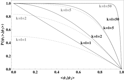

More quantitative insight into the behavior of and is presented in Figs. (1) and (2). The figure (1) illustrates that the more copies of the compared states we have and the smaller is their overlap, the higher is the probability of revealing the difference between the states. The overlap of a pair of randomly chosen states decreases with the dimension of . Therefore the mean probability for a fixed number of copies grows with the dimension . This fact is documented in Fig. (2).
II.3 Comparison with large number of copies
Let us now study the situation when and . In this case the sum in Eq. (12) has only two terms, which can be easily evaluated to obtain
| (19) | |||||
In this limit the same probability of success can be reached also by a different comparison strategy. We can first use the state reconstruction techniques to precisely determine the state and then by projecting the remaining state onto reveal the difference between the states.
For the limit, where the number of both compared states goes to infinity simultaneously (), from Eq. (13) we recover for any finite the classical behavior i.e.
| (20) |
Therefore we can conclude that larger the number of the copies and of the two states higher the probability to determine that the two states are different is. In the limit we essentially with a classical comparison problem.
III Comparison of coherent states
In any quantum information processing the prior knowledge about the system in which information is encoded plays an important role. The most explicit example one can name is the state estimation when the prior knowledge about the state is crucial. In what follows we will analyze the quantum state comparison and instead of assuming that the two compared states are totally arbitrary we will restrict a class of possible states. To be more specific, we will consider a harmonic oscillator and we focus our attention on comparison of coherent states.
Coherent states coherent are defined as eigenstates of the annihilation operator (acting on ) associated with eigenvalues taking arbitrary value in the complex plane, i.e. the set of coherent states is defined as
| (21) |
Our next task is two-fold: Firstly we introduce an optimal protocol for comparison of two coherent states. Secondly we propose an experimental realization of the optimal coherent states comparator. Following the same line of reasoning as in the previous section the measurement operator unambiguously revealing that the coherent states ( copies of state and copies of the state ) are different must obey the following “no-error” conditions
| (22) |
or equivalently
| (23) |
where is an arbitrary positive measure such that its support contains all coherent states.
Since the operators and are positive, the identity implies that their supports are orthogonal. As before (in the case of all pure states) it is optimal to choose to be a projector onto the orthocomplement of the support of . Denoting by the projector onto the support of we can write . As it is shown in Appendix C using a properly normalized Lebesgue measure on a complex plane we can write
| (24) |
Consider to be a general input state of the coherent-state comparison machine. Using the Eq.(24) we obtain the following expression for the success probability
| (25) | |||||
where we used the following modification of the rectangular identity
III.1 Optical setup for unambiguous comparison of coherent states
In this subsection we will describe an optical realization of an unambiguous coherent-states comparator that achieves the optimal value of the success probability (see above). The experimental setup we are going to propose will consist of several beam-splitters and only a single photodetector. A beam-splitter acts on a pair of coherent states in a very convenient way, in particular, the output beams remain unentangled and coherent, i.e.
| (26) |
where stand for transmissivity and reflectivity, respectively, and . The aforementioned property of the beam-splitter transformation enables us to consider each of its outputs separately.

Our setup is composed of beam-splitters and one photodetector. The beam-splitters are used to “concentrate” (focus) the information encoded in copies of the first state. Namely, they are arranged according to Fig. 3 and they perform the unitary transformation . To do this the transmissivities of the beam-splitters must be set as follows
Similarly, beam-splitters are used to “concentrate” the copies of the second state. The “concentrated” states , are then launched into the last beam-splitter in which the comparison of input coherent states is performed. It performs the following unitary transformation
| (27) | |||||
where is the reflectivity and transmissivity of the last beam-splitter. To obtain the vacuum in the upper output (see Fig.3) we need to adjust the values of reflectivity and transmissivity so that the identity holds, i.e.
Finally, a photodetector will measure the presence of photons in the upper output port of the last beam-splitter (see Fig. 3). If the two compared states are identical, in the output port we have zero photons - that is this port is in the vacuum state. Therefore a detection of at least one photon unambiguously indicates the difference between the compared states. On the other hand the observation of no photons is inconclusive, since each coherent state has a nonzero overlap with the vacuum. As a result we obtain the success probability
| (28) | |||||
which is the optimal one. Analyzing the last equation we find out that if and only if . This equivalence implies that . Thus, also in the case of coherent states the additional copy of one of the compared states helps to increase the mean success of the state comparison. For a fixed number of copies of both compared states the fraction is maximized for . Therefore, the probability of revealing the difference of the states is maximized if .
IV Conclusion
Let us summarize our main results on the quantum-state comparison derived in this paper. The difference of the unknown states can be unambiguously detected with the success rate
| (29) |
providing that we have copies of state and copies of the state . This result does not depend on the dimension of the system in contrast to the average success rate, which reads
| (30) |
Given the a priori knowledge that the states are coherent one can increase the probability (see Fig.1) to
| (31) |
The improvement is significant (Fig.1) for small number of copies.
We also addressed the problem of maximizing the success probability providing that the total number of available copies is fixed. We have shown that it is optimal if the number of copies is the same, i.e. . In the limit of the large number of copies the comparison approach reduces to “classical” comparison based on the quantum-state estimation.
We have proposed an optical implementation of the optimal quantum-state comparator of two finite ensembles of coherent states. This proposal is relatively easy to implement, since it consists only of beam-splitters and a single photodetector. Unfortunately, the success of unambiguous state comparison is very fragile with respect to small imperfections. The reason is that the device can be only used for pure states. Therefore our device can be used only in the situation when sources of a noise can be modeled as quantum channels preserving the validity of the no-error conditions . An example of such noise is an application of random unitary channel (simultaneously on all copies) transforming coherent states into coherent states.
ACKNOWLEDGMENTS
This work was supported by the European Union projects QAP, CONQUEST, by the Slovak Academy of Sciences via the project CE-PI, and by the projects APVT-99-012304, and VEGA. Authors want to thank Teiko Heinosaari for helpful discussions.
Appendix A Evaluation of
Before calculating the average of it is useful to evaluate the mean values of the overlaps
| (32) |
where we exploited the identity in Eq. (3).
Appendix B Proof of lemma
Lemma
Suppose we have a polynomial with the following properties:
-
1.
-
2.
for and for
Then for all .
Proof: For and it follows that . Therefore we can write
| (33) | |||||
| (34) | |||||
| (35) |
where we have used the fact that , i.e. .
Appendix C Projectors onto coherent states
Coherent states are intimately related to the group of phase-space displacements generated by the Glauber operator via the following relation , where is the vacuum (ground) state of a harmonic oscillator. Using the group invariant measure (its support contains all coherent states) the operator can be expressed as follows
| (36) |
Applying the theorem proved in Ref. shucker to the representation of the group of displacements we find that
| (37) |
where is a positive number ( is positive) and is the projector onto the linear subspace spanned by the product states . A particular choice of the group invariant measure affects the value of the parameter . Our goal is to calculate the projector , hence we are looking for a measure such that . The canonical Lebesgue measure on the complex plane is invariant under complex translations (displacements) and therefore the correct measure is proportional to , that is for some positive number , i.e.
| (38) |
Now, setting , we have, expanding the coherent states in terms of number states,
| (39) | |||||
because if , and vanishes otherwise. The invariance of the canonical Lebesgue measure implies that
| (40) | |||||
The previous identity (40) implies
| (41) |
Consequently, for all it holds that
| (42) |
and for all we have . The above equality fixes the invariant measure to be , where is the Lebesgue measure on the complex plane.
References
- (1) S.M. Barnett, A. Chefles, and I. Jex, Phys. Lett. A 307, 189 (2003).
- (2) A.Chefles, E. Andersson, and I. Jex, J. Phys. A: Math. Gen. 37, 7315 (2004).
- (3) M. Kleinmann, H. Kampermann, and D. Bruss, Phys. Rev. A 72, 032308 (2005).
- (4) E. Andersson, M. Curty, and I. Jex, Phys. Rev. A 74, 022304 (2006).
- (5) M.A.Nielsen and I.L.Chuang, Quantum Computation and Quantum Information (Cambridge University Press, Cambridge, 2000).
- (6) A. Hayashi, T. Hashimoto, and M. Horibe, Phys. Rev. A 72, 032325 (2005).
- (7) M.O. Scully and M.S. Zuhairy, Quantum Optics (Cambridge University Press, Cambridge, 1997).
- (8) D.S.Shucker, Proc. of the American Mathematical Society 89, 169 (1983).