The influence of residual gas expulsion on the evolution of the Galactic globular cluster system and the origin of the Population II halo

Abstract

We present new results on the evolution of the mass function of the globular cluster system of the Milky Way, taking the effect of residual gas expulsion into account. We assume that gas embedded star clusters start with a power-law mass function with slope $\beta=2$, similar to what is observed for the Galactic open clusters and young, massive star clusters in interacting galaxies. The dissolution of the clusters is then studied under the combined influence of residual gas expulsion driven by energy feedback from massive stars, stellar mass-loss, two-body relaxation and an external tidal field. The influence of residual gas expulsion is studied by applying results from a large grid of $N$-body simulations computed by Baumgardt & Kroupa (2007).

In our model, star clusters with masses less than $10^{5}M_{\odot}$ lose their residual gas on timescales much shorter than their crossing time and residual gas expulsion is the main dissolution mechanism for star clusters, destroying about 95% of all clusters within a few 10s of Myr. We find that in this case the final mass function of globular clusters is established mainly by the gas expulsion and therefore nearly independent of the strength of the external tidal field, and that a power-law mass function for the gas embedded star clusters is turned into a present-day log-normal one, verifying the theory proposed by Kroupa & Boily (2002). Our model provides a natural explanation for the observed (near-)universality of the peak of the globular cluster mass function within a galaxy and among different galaxies. Our simulations also show that globular clusters must have started a factor of a few more concentrated than as we see them today.

Another consequence of residual gas expulsion and the associated strong infant mortality of star clusters is that the Galactic halo stars come from dissolved star clusters. Since field halo stars would come mainly from low-mass, short-lived clusters, our model would provide an explanation for the observed abundance variations of light elements among globular cluster stars and the absence of such variations among the halo field stars. Furthermore, our modelling suggests a natural tendency of $>10^{7}\mbox{M}_{\odot}$ gas clouds to retain their residual gas despite multiple supernova events, possibly explaining the complex stellar populations observed in the most massive globular clusters.

1 Introduction

Globular clusters are among the oldest components of galaxies, having formed within a few hundred Myr after the Big Bang (Chaboyer et al., 1998; VandenBerg et al., 2002; Gratton et al., 2003). Observations of globular cluster systems in galaxies can therefore bring important insights about star formation in the early universe and the formation and early evolution of galaxies. One of the most remarkable properties of globular cluster systems is their mass distribution. Observations of the Milky Way and other nearby galaxies show that globular clusters follow a bell shaped distribution in luminosity with an average magnitude of $M^{0}_{V}\approx-7.3$ and dispersion $\sigma_{V}=1.2$ (Harris, 1991). For a mass-to-light ratio of $M/L_{V}=1.5$, this corresponds to a characteristic mass of $1.1\cdot 10^{5}M_{\odot}$. The peak of the globular cluster luminosity function (GCLF) appears to be remarkably similar between different galaxies (Harris, 1991; Secker, 1992; Kundu & Whitmore, 2001a, b; Nantais et al., 2006) and also at different radii within individual galaxies (Kavelaars & Hanes, 1997; Harris, Harris & McLaughlin, 1998; Tamura et al., 2006), although evidence for a fainter peak of the GCLF in dwarf galaxies has recently been reported (Jórdan et al., 2006; van den Bergh, 2006). These findings pose strong constraints on any theory of globular cluster formation and their later dynamical evolution.

Their bell-shaped luminosity function sets globular clusters apart from young, massive star clusters in starburst and interacting galaxies (Whitmore & Schweizer, 1995; Whitmore et al., 1999; Fall & Zhang, 1999; Larsen, 2002; Whitmore et al., 2002; de Grijs et al., 2003) and the open clusters of the Milky Way and other nearby spiral galaxies (Fuente Marcos & Fuente Marcos, 2004; Gieles et al., 2006), which generally follow a power-law distribution over luminosities down to the faintest observable clusters. The question arises whether the luminosity function of globular clusters is of primordial origin, such that the turnover mass is related to a primordial Jeans mass (Fall & Rees, 1985), or whether globular clusters also started with a power-law mass function and the present-day peak is due to the quicker dynamical evolution and preferential destruction of the low-mass clusters.

Okazaki & Tosa (1995) and Baumgardt (1998) studied the evolution of the Galactic globular cluster system under the combined influence of two-body relaxation, mass segregation and an external tidal field and concluded that an initial power-law mass function $dN/dM_{C}\sim M_{C}^{-\beta}$ with slope $\beta\sim 2.0$ can, over the course of a Hubble time, be turned into a bell-shaped mass function with parameters similar to what is observed for globular clusters. Using more realistic modelling of the lifetimes, Vesperini (1998, 2000), on the other hand, pointed out that an initial power-law mass-function cannot evolve to the observed bell-shaped form, but that an initial log-normal shape of the mass function similar to the observed one is preserved by the dynamical evolution, offering an alternative way to explain the near-uniformity of the GCLF. Vesperini (2001) and Parmentier & Gilmore (2005) also showed that power-law initial mass functions generally lead to radial gradients in the peak of the mass function.

Fall & Zhang (2001) found that an initial velocity distribution which is radially anisotropic and where the amount of radial anisotropy increases with galactocentric distance is able to destroy a radial gradient in the shape of the mass function. However, Vesperini et al. (2003) analysed the M87 globular cluster system and, while they found that a strong radial anisotropy increasing with galactocentric distance would be able to reproduce the observed constancy of the peak of the mass function at all radii, they also showed that such strongly radially anisotropic distributions are inconsistent with the observed kinematics of the M87 globular clusters, calling into question whether globular clusters really formed with power-law mass functions. Parmentier & Gilmore (2007) finally studied the influence of residual gas expulsion and found that a system of protoglobular clouds with a mean mass of $M_{Cl}=10^{6}\mbox{M}_{\odot}$ results in a Gaussian cluster mass function with the appropriate turnover at the end of the gas expulsion phase. That shape is then preserved by the subsequent dynamical evolution, thus satisfying observational constraints.

While the above mentioned papers considered the influence of two-body relaxation, external tidal fields and dynamical friction on the dissolution of star clusters, with the exception of Kroupa & Boily (2002) and Parmentier & Gilmore (2007), all papers neglected the influence of residual gas expulsion. However, there is ample observational evidence that residual gas expulsion is an important mechanism in the early evolution of star clusters: Lada & Lada (2003) for example studied embedded star clusters in the solar neighbourhood and found that less than 4% - 7% of the embedded star clusters survive the initial gas removal to become bound clusters of Pleiades age. Even for the surviving ones, Weidner et al. (2007) found that they lose of order 50% of their stars due to gas expulsion. A similar steep decline of the number of clusters with age was also found by Chandar, Fall & Whitmore (2006) for star clusters in the SMC (see however Gieles, Lamers & Portegies Zwart (2006) who attribute this decline to detection incompleteness). In addition, Bastian & Goodwin (2006) found that the luminosity profiles of young, massive star clusters in several dwarf galaxies can best be understood by clusters which have undergone a rapid removal of a significant fraction of their mass as a result of gas expulsion. Finally, the majority of OB stars in the Milky Way and other nearby galaxies are found in unbound associations (Pellerin et al., 2006), which, together with the assumption that stars form in clusters, again points to the rapid dissolution of most clusters within 10 Myr. Since two-body relaxation or tidal shocks dissolve clusters only relatively slowly, such observations point to residual gas expulsion as the main process for the dissolution of star clusters, as summarised and stressed by Kroupa (2005) (see also Baumgardt & Kroupa (2007) for a summary of analytic and numerical studies on residual gas expulsion).

The present paper is the eighth paper in a series which explores the influence of residual gas expulsion on the dynamical evolution of star clusters and star cluster systems (Kroupa, Petr & McCaughrean, 1999; Kroupa, 2000; Kroupa, Aarseth & Hurley, 2001; Kroupa, 2002; Kroupa & Boily, 2002; Boily & Kroupa, 2003a, b; Baumgardt & Kroupa, 2007). In the most recent paper (Baumgardt & Kroupa, 2007), we have performed a large set of $N$-body simulations studying residual gas expulsion and the subsequent reaction of the star cluster to the drop in cluster potential. We varied the star formation efficiency, gas expulsion timescale and strength of the external tidal field and obtained a three-dimensional grid of models which can be used to predict the evolution of individual star clusters or whole star cluster systems by interpolating between our runs. Here, we apply these results to the globular cluster system of the Milky Way in order to derive constraints on the initial properties of the Galactic globular cluster system. In a companion paper (Parmentier et al., 2008), we will focus on the shape of the mass function of young clusters which have survived gas expulsion, and study how this shape responds to variations in the local SFE.

In this contribution, we address two key findings deduced by Kroupa & Boily (2002), namely that residual gas expulsion (i) re-shapes the cluster MF within $\leq 100$ Myr and (ii) that the Galactic population II stellar halo naturally results from infant cluster mortality, thereby being physically related to the globular cluster population in terms of stemming from the low-mass clusters formed at the same time (Larsen, 2004). These results were arrived at using analytical work. Here we return to these with the help of the currently largest existing $N$-body library of cluster evolution under residual gas expulsion (Baumgardt & Kroupa, 2007). The paper is organised as follows: In Sec. 2 we describe our model for the initial cluster distribution and our assumption for the various destruction mechanisms. Sec. 3 describes the results and in Sec. 4 we draw our conclusions.

2 The models

2.1 Initial cluster properties

We assume that pre-cluster molecular cloud cores are distributed with a power-law mass function $dN/dM_{Cl}\sim M_{Cl}^{-\beta_{Cl}}$ between lower and upper mass limits of $M_{Low}=10^{3}M_{\odot}$ and $M_{Up}=10^{8}M_{\odot}$. Including cores with masses below $10^{3}M_{\odot}$ would not change our results since the clusters formed out of such low-mass cores are destroyed by dynamical evolution. Most simulations were made with a power-law index $\beta_{Cl}=2.0$, similar to the observed slopes for young star clusters in nearby and starburst galaxies.

The star formation efficiencies $\epsilon$ are assumed to follow a Gaussian distribution with a mean of 25% and a dispersion of 5%. Such a distribution is in agreement with observed star formation efficiencies which generally have $\epsilon\mathrel{\mathop{\!\!\!\!\begin{array}[]{c}<\\ \sim\end{array}}\!\!\!}40$% (Lada & Lada, 2003). No correlation of the SFE with cloud core mass is assumed and the gas embedded cluster masses are calculated according to $M_{ecl}=\epsilon M_{Cl}$ such that $\beta=\beta_{Cl}$. We assume that star clusters are in virial equilibrium prior to gas expulsion. Assuming an initially cold or hot velocity distribution for the stars would change the impact of gas expulsion and the survival limits (see e.g. Verschueren (1990); Goodwin & Bastian (2006)). However, dynamically cold systems can probably be excluded for the majority of clusters since the strong impact that gas expulsion has on cluster systems would be hard to explain with them, at least as long as typical SFEs are of order 30%. The pre-gas expulsion cluster radii are assumed to follow a Gaussian distribution with width $\log(\sigma_{R}/\mbox{pc})=0.2$ and various means given by $\log(r_{h}/\mbox{pc})=\log(r_{hm}/\mbox{pc})+k_{r}\log(R_{G}/\mbox{kpc})$, i.e. our distributions are allowed to change with Galactocentric distance (note that $\log=\log_{10}$).

The number density distribution of clusters in the Milky Way before gas expulsion is given by:

$$\rho(R_{G})\sim\left(1+\frac{R_{G}^{2}}{R_{Core}^{2}}\right)^{-\alpha_{G}/2}\;\;,$$ (1)

where $R_{G}$ is the Galactocentric distance and $R_{Core}$ the core radius of the cluster distribution, which was set to $R_{Core}=1\;\mbox{kpc.}$ Most simulations were done with either $\alpha_{G}=3.5$ or $\alpha_{G}=4.5$.

We treat the Milky Way as a spherical system with constant rotation velocity $V_{C}=220$ km/s and distribute the clusters spherically symmetric according to the chosen density profile. Cluster velocities were assigned according to a chosen global anisotropy $\beta_{v}$ of the cluster system, defined by

$$\beta_{v}=1-\frac{\sum(v^{2}_{\theta}+v^{2}_{\phi})}{2\sum v^{2}_{r}}\;\;\;,$$ (2)

where $v_{\theta}$, $v_{\phi}$ and $v_{r}$ are the two tangential velocities and the radial velocity of each cluster and the sums run over all clusters. Most simulations were done with isotropic ($\beta_{v}=0$) or mildly radially anisotropic ($\beta_{v}=0.5$) velocity dispersions. After setting up the clusters, we calculated the peri- and apocenter distances and the orbital period for each cluster in order to be able to estimate the influence of the various destruction mechanisms.

2.2 Destruction mechanisms

2.2.1 Gas expulsion

Gas expulsion was modelled by interpolating between the grid of runs made by Baumgardt & Kroupa (2007). In order to use their simulation grid, the ratio of the gas expulsion time scale to the cluster’s crossing time, $\tau_{M}/t_{Cross}$, the ratio of the cluster’s half-mass radius to its tidal radius, $r_{h}/r_{t}$, and the star formation efficiency, $\epsilon$ have to specified. The star formation efficiency, $\epsilon$, and half-mass radius, $r_{h}$, were already chosen when the cluster system was set up. The crossing time, $t_{Cross}$, is calculated from the pre-gas expulsion cloud core mass $M_{Cl}$, and virial radius, $r_{v}$, according to

$$t_{Cross}=2.82\sqrt{\frac{r_{v}^{3}}{GM_{Cl}}}\;\;.$$ (3)

We assume $r_{v}=1.30r_{h}$, which is the relation for a Plummer model. If we neglect contributions coming from the ellipticity of the cluster orbit, the tidal radius of a cluster with mass $M_{ecl}$, moving through an isothermal Galactic potential with pericenter distance, $R_{P}$, is (Innanen, Harris & Webbink, 1983)

$$r_{t} = \left(\frac{M_{ecl}}{2M_{G}(<R_{P})}\right)^{1/3}R_{P}$$ (4)

$$= \left(\frac{GM_{ecl}}{2V_{C}^{2}}\right)^{1/3}R^{2/3}_{P}$$

The model for the gas expulsion timescale $\tau_{M}$ will be described in Sec. 3.2 below.

Once values for all three parameters are specified, the fate of each cluster was calculated by linearly interpolating between the grid points of Baumgardt & Kroupa (2007). Interpolation was done by using the 8 grid points surrounding the position of each cluster. Linear interpolation between these points in one coordinate, for example $\epsilon$, creates 4 data points with the same SFE as the cluster. A second linear interpolation between these 4 points in another coordinate reduces them to two data points and a final interpolation between these in the third coordinate gives a prediction for the surviving mass and final half-mass radius of the cluster. If 5 or more of the 8 grid points surrounding the position of a cluster correspond to dissolved clusters, the cluster was also assumed to be dissolved due to gas expulsion. The final cluster radius was determined similarly, except that interpolation was done only if both points correspond to surviving clusters.

For clusters for which the parameter values are outside the range considered by Baumgardt & Kroupa (2007), the above procedure is not applicable. In this case we assumed that clusters with $\epsilon<0.05$ or $r_{h}/r_{t}>0.2$ will not survive, as indicated by the simulations of Baumgardt & Kroupa (2007), while clusters with $r_{h}/r_{t}<0.01$ or $\tau_{M}/t_{Cross}>10.0$ were assumed to follow the same evolution as clusters with $r_{h}/r_{t}=0.01$ and $\tau_{M}/t_{Cross}=10.0$ respectively.

2.2.2 Stellar evolution

Stellar evolution reduces the masses of star clusters by about 30% over the course of a Hubble time (Baumgardt & Makino, 2003). Most of this mass loss happens within the first 100 Myr after cluster formation. We therefore applied stellar evolution mass loss after gas expulsion and before the other mechanisms. Mass loss due to stellar evolution also causes the clusters to expand. We assumed that the expansion is happening adiabatically since the timescale for mass loss due to post gas-expulsion stellar evolution is much longer than the crossing time of star clusters, and increased the cluster radii by a factor $r_{hf}/r_{hi}=1/0.7=1.43$ (Hills, 1980).

2.2.3 Two-body relaxation and the Galactic tidal field

The effects of two-body relaxation and a spherical external tidal field were modelled according to the results of Baumgardt & Makino (2003), who performed simulations of multi-mass clusters moving through spherically symmetric, isothermal galaxies. According to Baumgardt & Makino (2003), the time until disruption, or lifetime, of a star cluster moving through an external galaxy with circular velocity $V_{C}$ on an orbit with pericenter distance $R_{P}$ and eccentricity $\epsilon$ is given by

$$\frac{t_{DisR}}{\mbox{[Myr]}}=k\left(\frac{N}{ln(0.02\,N)}\right)^{x}\!\!\frac{R_{P}}{\mbox{[kpc]}}\left(\frac{V_{C}}{220\mbox{km/s}}\right)^{-1}\!\!\!\!(1+\epsilon)\,.$$

Here $N$ is the number of cluster stars left after gas expulsion, which can be calculated from the cluster mass after gas expulsion and the mean mass of the cluster stars as $N=M_{0}/\!\!<\!m\!>$. A standard Kroupa (2001) IMF between mass limits of 0.1 and 15 $M_{\odot}$ has $<\!m\!>=0.547$ M_⊙. $x$ and $k$ are constants describing the dissolution process and are given by $x=0.75$ and $k=1.91$ (Baumgardt & Makino, 2003). An exponent $x$ flatter than unity is also indicated by the observations of Boutloukos & Lamers (2003).

2.2.4 Disc shocks

Since the simulations of Baumgardt & Makino (2003) did not take into account the effects of passages through galactic discs, we have to add these separately to our simulations. According to Ostriker, Spitzer, & Chevalier (1972) and Binney & Tremaine (1987), the time it takes for stars to increase their energy by an amount equal to their typical energy is given by

$$t_{Shock}=\frac{T_{\psi}\;\sigma^{2}\;V^{2}_{\perp}}{8\bar{z^{2}}\bar{g_{z}^{2}}}\;\;.$$ (5)

Here $T_{\psi}$ is the azimuthal period of the orbit, taken to be equal to the orbital period, $\sigma$ is the internal velocity dispersion of the cluster, $V_{\perp}$ is the velocity of the cluster relative to the disc at the time of the passage, $\bar{z^{2}}$ is the average square-$z$ expansion of the stars in the cluster and $g_{z}$ is the vertical component of the gravitational field of the galaxy at the point where the cluster crosses the disc. $\sigma^{2}$ and $\bar{z^{2}}$ can be calculated from the clusters half-mass radius and mass according to $\sigma^{2}=0.4GM_{0}/r_{h}$ and $\bar{z^{2}}=\frac{1}{3}r_{h}^{2}$. For exponential discs, $g_{z}$ can be approximated by $g_{z}=2\pi G\Sigma_{0}exp(R/R_{d})$ (Binney & Tremaine, 1987), where $\Sigma_{0}=750.0M_{\odot}/\mbox{pc}^{2}$ is the surface density of the Galactic disc and $R_{d}=3.5$ kpc its scale length. In order to obtain $t_{Shock}$, we calculated $V_{\perp}$ and $g_{z}$ for pericenter and apocenter passages separately and summed up their contributions. The dissolution time for a cluster evolving under both relaxation and disc shocking was assumed to be

$$\frac{1}{t_{DisT}}=\frac{1}{t_{DisR}}+\frac{1}{t_{Shock}}\;\;.$$ (6)

We assumed that the mass is lost linearly over the lifetime of a cluster, so the mass remaining at a time $t<t_{DisT}$ is given by

$$M_{C}(t)=0.7\,M_{0}\,(1-t/t_{DisT})\;\;,$$ (7)

where the factor 0.7 takes into account the mass lost from clusters due to stellar evolution and $M_{0}$ is the cluster mass after gas expulsion induced loss of stars.

2.2.5 Dynamical friction

Massive clusters in the inner parts of galaxies spiral into the centres due to dynamical friction (Spitzer, 1969; Tremaine, Ostriker & Spitzer, 1975). According to Binney & Tremaine (1987), the time to reach the galactic centre for a cluster of mass $M_{0}$ and initial distance $R_{G}$ is given by:

$$\frac{t_{Fric}}{yr}=\frac{2.64\cdot 10^{11}}{\ln\Lambda}\left(\frac{R_{G}}{2kpc}\right)^{2}\left(\frac{V_{C}}{250km/s}\right)\left(\frac{10^{6}M_{\odot}}{M_{0}}\right)$$ (8)

In our calculations, we used $\ln\Lambda$ = 10. We computed for all clusters the friction time scale after applying gas expulsion and destroyed those with $t_{fric}<T_{Hubble}$. We used the semi-major axis of each cluster’s orbit as the distance to the galactic centre. For the surviving clusters, their orbital parameters were reduced according to

$$R_{G\;f}=R_{G\;i}\sqrt{1-\frac{T_{Hubble}}{t_{Fric}}}\;\;,$$ (9)

which follows from eq. 7-28 of Binney & Tremaine (1987). We assumed no change of orbital eccentricity due to dynamical friction and neglected changes in the efficiency of dynamical friction due to the mass loss of the clusters. We also neglected changes in the shocking timescale due to the inspiral.

We followed the evolution of the cluster system for a Hubble time, assumed to be $T_{Hubble}=13$ Gyr. Clusters were destroyed if either $t_{DisT}<T_{Hubble}$ or $t_{Fric}<T_{Hubble}$ or if the clusters half-mass radius was larger than 33% of the perigalactic tidal radius after a Hubble time.

3 Results

3.1 Runs without gas expulsion

We first discuss the results of runs without residual gas expulsion. As a starting case, we assume a cluster distribution with $\alpha_{G}=4.5$, power-law mass function index $\beta=2.0$ and mean cluster radius $\log(r_{h}/\mbox{pc})=0.3+0.2\log(R_{G}/\mbox{kpc})$. This distribution will henceforth be referred to as the standard case. Fig. 1 depicts the surviving mass distribution of clusters when we split up our sample into inner clusters which have Galactocentric distances $R_{G}<8$ kpc and outer clusters with $R_{G}>8$ kpc at the end of the simulation, and compares it with the sample of Milky Way globular clusters, taken from Harris (1996). It can be seen that the final distribution for clusters inside 8 kpc (solid line) is in rough agreement with the observations (points), since both distributions have a maximum around $10^{5}M_{\odot}$. This is due to efficient cluster destruction as a result of the strong tidal field in the inner galaxy, which reduces the number of clusters with masses $M_{C}=10^{3}$ M_⊙ by several orders of magnitude. However, the distribution of outer clusters is in contrast to the observations since, while the observations show a turnover near $10^{5}M_{\odot}$, the simulated distribution is still rising towards the smallest studied cluster masses due to the weak tidal field in the outer parts of the Milky Way. Since the observed mass distribution for clusters with masses $M_{C}>10^{4}M_{\odot}$ is likely to be complete, the mismatch cannot be due to incompleteness, but must be due to our assumptions.

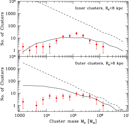
Figure 1: Initial (dashed lines) and surviving (solid lines) mass distribution of star clusters in case of no gas expulsion for clusters with Galactocentric distances $R_{G}<8$ kpc and clusters with $R_{G}>8$ kpc, compared to the observed distribution of Milky Way clusters from Harris (1996) (points). While the distribution of inner clusters is in rough agreement with the observations, too many low-mass clusters survive in the outer parts, due to the weak tidal field.

Varying the initial cluster distribution also does not help in reconciling this difference (Fig. 2). For example, changing the cluster orbits from an isotropic distribution to a radially anisotropic distribution with $\beta_{v}=0.5$, or by choosing a flatter radial density distribution of the clusters in the galaxy has an almost negligible influence on the final mass distribution. The mismatch with the observations can be reduced if the initial power-law index $\beta$ is decreased, since in this case a smaller number of low-mass clusters form initially. However, the number of high mass clusters with masses $M_{C}>10^{6}M_{\odot}$ is significantly overpredicted in this case. In addition, observed power-law distributions have generally $\beta=1.8$ or larger. Changing the distribution of cluster radii to a distribution with radii $<\!\log{r_{h}}\!>=0.5$, independent of Galactocentric distance, also has nearly no influence on the final mass distribution.

All models discussed so far predict a strong change of average cluster mass with Galactocentric radius due to the fact that cluster dissolution through either relaxation or external tidal shocks depends on the strength of the external tidal field. This variation is however not observed in either the Milky Way or external galaxies (Kavelaars & Hanes, 1997; Jórdan et al., 2006), at least not with the predicted strength. Hence, the observed peak cannot be caused by these processes but must be either primordial or due to a different dissolution process.

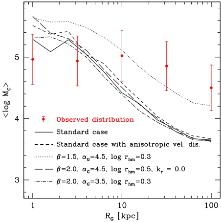
Figure 2: Mean mass $<\!logM_{C}\!>$ of the model clusters compared to the observed distribution of Milky Way clusters for different initial conditions for the case of no residual gas expulsion (i.e. $\epsilon=1$). The standard case (solid line) has $\alpha_{G}=4.5$, $\log r_{hm}=0.3$ and $\beta=2.0$ and clusters on isotropic orbits. All other runs vary the initial conditions: Clusters on radially anisotropic orbits with $\beta_{v}=0.5$ (short dashed), a flatter mass spectrum of embedded clusters with $\beta=1.5$ (dotted), clusters with larger half-mass radii $\log r_{hm}=0.5$ independent of Galactocentric distance ($k_{r}=0$, long dashed), and clusters with a flatter radial distribution in the galaxy $\alpha_{G}=3.5$ (dashed-dotted). In all cases, a decrease of the mean mass with Galactocentric distance is predicted which is not observed.

These conclusions agree with Vesperini (2001) and Parmentier & Gilmore (2005), but are in disagreement to Fall & Zhang (2001) and McLaughlin & Fall (2007). The reason for this discrepancy is that Fall & Zhang (2001) studied clusters on highly radial orbits which are ruled out observationally at least for M87 (Vesperini et al., 2003). McLaughlin & Fall (2007) on the other hand assumed dissolution times which are independent of the strength of the external tidal field, which is ruled out by simulations which show that isolated clusters don’t dissolve at all (Baumgardt, Hut & Heggie, 2002), while for clusters in tidal fields the dissolution time depends on the strength of the external tidal field (Gnedin & Ostriker, 1996; Vesperini & Heggie, 1997; Baumgardt, 2001; Baumgardt & Makino, 2003; Lamers, Gieles & Portegies Zwart, 2005).

As already explained in the Introduction, gas expulsion is an excellent candidate for a process which is (nearly) independent of the strength of the external tidal field, and we will study its influence in the next section.

3.2 A model for residual gas expulsion

Neglecting the influence of the surrounding interstellar medium (ISM), gas from a cluster can only be lost if the total energy put into a gas cloud by OB stars exceeds the potential energy of the cloud. The potential energy of a gas cloud with radius $r$, mass $M_{Cl}$ and star formation efficiency $\epsilon$ is given by

$$E_{Gas}=k(1-\epsilon)\frac{G\;M^{2}_{Cl}}{r}\;\;,$$ (10)

where the factor $(1-\epsilon)$ accounts for the fact that some gas was transformed into stars. For $r=r_{h}$ and a Plummer model, the dimensionless constant $k$ is approximately $k\approx 0.4$. The energy $E_{Gas}$ is the minimum energy which has to be injected into a gas cloud in order to disperse it. According to the simulations by Freyer, Hensler & Yorke (2006), who studied energy-deposition of stellar feedback into gas clouds, a star of mass $m=35M_{\odot}$ puts an energy of $\dot{E}=6.7\cdot 10^{49}$ erg/Myr into the ISM in the form of radiation and mechanical energy. Corresponding values for $m=60M_{\odot}$ ($85M_{\odot}$) stars are $\dot{E}=1.8\cdot 10^{50}$ ($\dot{E}=3.4\cdot 10^{50}$) erg/Myr (Freyer, Hensler & Yorke, 2003; Kroeger et al., 2007). The above values can be fitted with

$$\log_{10}{\dot{E_{*}}}/\mbox{erg/Myr}=50.0+1.72\cdot(\log_{10}m/M_{\odot}-1.55)\;\;.$$ (11)

Integrating this over all stars in a cluster, assuming a canonical IMF (Kroupa, 2001) between 0.1 and 120 $M_{\odot}$, gives for the total energy input of a cloud of mass $M_{Cl}$:

$$\dot{E} = \epsilon M_{Cl}\int_{0.1M_{\odot}}^{120M_{\odot}}\dot{E}_{*}N(m)dm$$ (12)

$$= 2.5\cdot 10^{4}\;\epsilon\;M_{Cl}\;\mbox{M}_{\odot}\mbox{km}^{2}\mbox{/s}^{2}/\mbox{Myr}\;\;.$$

If we compare this with the total potential energy of the cloud, we obtain as an estimate for the gas expulsion timescale $\tau_{M}$ (defined in eq. 3 of Baumgardt & Kroupa (2007)):

$$\tau_{M}=E_{Gas}/\dot{E}=7.1\cdot 10^{-8}\;\frac{1-\epsilon}{\epsilon}\frac{M_{Cl}}{[M_{\odot}]}\left(\frac{r_{h}}{[pc]}\right)^{-1}\mbox{Myr}.$$ (13)

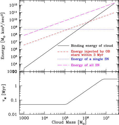
Figure 3: Energy of a gas cloud (solid line) vs. cloud mass $M_{Cl}$ in comparison with the energy input from OB stars (short dashed) and the energy input by supernova explosions (dotted and long dashed) for a gas cloud with a half-mass radius $r_{h}=0.5$ pc and SFE of 25% (top panel) and the resulting gas expulsion time scale $\tau_{M}$ (bottom panel) used in this paper. OB stars eject enough energy to disperse gas clouds with masses up to $10^{6}M_{\odot}$ within 3 Myr. More massive clouds are dispersed by supernova explosions. For the most massive clouds with $M_{Cl}>10^{7}M_{\odot}$, the potential energy of the gas cloud can exceed the combined energy of all supernova explosions, meaning that some fraction of the supernova ejecta will be retained. This raises the possibility of multiple star-formation events in these systems. The resulting gas expulsion timescales for a star cluster with $\epsilon=0.25$ and $r_{h}=0.5$ pc vary between $5\cdot 10^{4}$ yrs and 3 Myrs.

In very massive systems, the above formula leads to gas expulsion timescales in excess of 3 Myr, so supernova explosions also become important in removing the gas. If we assume that a typical supernova explosion ejects around $1\cdot 10^{51}$ erg into the ISM, the total energy ejected by supernovae is given by:

$$E_{SN}=5.025\cdot 10^{7}\;\epsilon\;f_{SN}\;M_{Cl}\;\mbox{M}_{\odot}\mbox{km}^{2}\mbox{/s}^{2}\;\;.$$ (14)

Here $f_{SN}$ is the fraction of all stars with mass $m>8$ M_⊙ and which undergo supernova explosions. For a Kroupa IMF from 0.1 to 120 $M_{\odot}$, $f_{SN}=0.0061$. Fig. 3 depicts the energy input of OB stars and supernova explosions into the ISM for gas embedded clusters with a half-mass radius of 0.5 pc and SFE $\epsilon=0.25$. It can be seen that OB stars eject enough energy to disperse gas clouds with masses up to $10^{6}M_{\odot}$ within 3 Myr, i.e. before the first supernova explosions go off. The first supernova (assumed to have an energy of $5\cdot 10^{51}$ erg) going off in a cluster ejects an energy amount small compared to what OB stars already injected and is thus unlikely to have a strong impact on the cluster gas. However, the combined energy input from all supernovae is about one order of magnitude larger than what OB stars eject and is strong enough to disperse even clouds with masses up to $10^{7}M_{\odot}$.

For the most massive clouds, the total energy injected into the ISM is however only slightly larger than the cloud binding energy. Some gas from supernova explosions might therefore be retained in such clouds and form a second generation of stars enriched in heavy elements. Interestingly, in the mass range $M_{C}>few\cdot 10^{6}$ M_⊙ multiple stellar populations are observed in Local Group clusters like $\omega$ Cen (Hilker & Richtler, 2000; Piotto et al., 2005) and G1 (Meylan et al., 2001). It is also the mass range where a transition from globular clusters to UCDs is observed (Evstigneeva et al., 2007; Dabringhausen et al., 2008). According to Fig. 3, insufficient gas removal and multiple star-formation events could be one reason for the differences of heavy clusters to ordinary GCs.

Based on Fig. 3, we therefore choose $\tau_{M}$ from eq. 13 for the gas expulsion timescale if $\tau_{M}$ is smaller than 3 Myr. For larger gas clouds we assume $\tau_{M}=3$ Myr. For low-mass clouds, the finite time the gas needs to leave the cluster also becomes important. If we assume that the gas is leaving with the sound speed of the ISM ($v_{s}\approx 10$ km/s), we obtain a lower limit for the gas removal timescale of

$$\tau_{M}=\frac{r_{h}}{v_{s}}=0.098\;\frac{r_{h}}{\mbox{[pc]}}\ \;\mbox{Myr}\;\;\;.$$ (15)

Fig. 3 depicts the resulting gas expulsion timescales for a gas cloud with $\epsilon=0.25$ and $r_{h}=0.5$ pc.

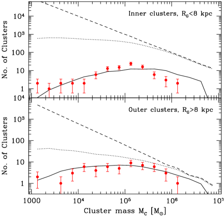
Figure 4: Mass distribution of star clusters before gas expulsion (dashed lines, the ”embedded cluster MF”), after gas expulsion (dotted lines, the ”initial cluster MF”) and after a Hubble time (solid lines), compared to the observed distribution of Milky Way clusters (points). Most low-mass clusters are destroyed by residual gas expulsion. The distribution of surviving clusters is now in good agreement with the observed one for both inner and outer clusters.

3.3 Runs including residual gas expulsion

We make the following assumptions for our standard case: SFEs follow a mass-independent Gaussian distribution with a mean of 25% and a dispersion of 5%. The effect that other SFE distributions have on the shape of the final cluster distribution will be discussed in more detail in a forthcoming paper (Parmentier et al., 2008). The spatial distribution of the clusters in the galaxy has a power-law exponent of $\alpha_{G}=4.5$, the power-law mass function index is $\beta=2.0$ and mean initial cluster radii follow a relation $\log_{10}r_{h}/\mbox{pc}=-0.1+0.2\cdot\log_{10}R_{G}/\mbox{kpc}$.

Fig. 4 depicts the evolution of the mass function of clusters if we include gas removal into the runs. After gas expulsion, the number of low-mass clusters is decreased by a factor of 10 to 100, but still continues to rise towards low-masses. Massive clusters are not strongly effected by gas expulsion due to the large ratio of $\tau_{M}/t_{cross}$, so their number is close to the initial one and the slope at the high-mass end flattens only slightly. In total, only 3% of all clusters survive residual gas expulsion in this case. Due to the efficient destruction of low-mass clusters, the overall mass function after a Hubble time is in good agreement with the observed one for both inner and outer star clusters.

The main remaining difference to the observations is that our runs overpredict the number of high-mass clusters. This could be removed in a number of ways, like assuming shorter gas removal times for high-mass clusters or that the mass function of high-mass clusters in the Milky Way was truncated around $10^{6}$ M_⊙ (Gieles et al., 2006), due, for example, to star formation rates which were not high enough to allow the formation of more massive clusters (Weidner et al., 2004). Also, the mass function of embedded clusters could have been steeper (Weidner et al., 2004).

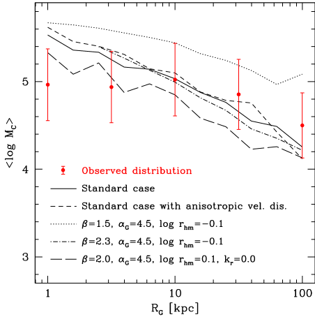
Figure 5: Mean masses $<\!logM_{C}\!>$ of the simulated clusters in runs with gas expulsion compared to the observed distribution of Milky Way clusters. The standard distribution (solid line) predicts average masses which are in agreement with observations at all Galactocentric distances. Assuming radial anisotropic orbits (short dashed) makes little difference to the final mass function. Larger initial cluster radii decrease the average masses of clusters at all radii (long dashed) while steeper embedded mass-functions lead to too many low-mass clusters surviving at large radii (dot-dashed) and flatter embedded mass-functions overpredict the average cluster mass at all radii (dotted).

The good agreement is confirmed by Fig. 5, which shows the average cluster mass as a function of Galactocentric distance. For our standard model, the average cluster mass decreases only slightly with Galactocentric distance, and stays for most distances within the limits observed for Milky Way globular clusters. The dispersion is also close to the observed one and exceeds it only at small Galactocentric radii. Changing the velocity dispersion of the globular cluster system from isotropic to radially anisotropic orbits with $\beta_{v}=0.5$ (dashed lines) leads to average cluster masses which are slightly larger than in the isotropic case. The differences are however small. Similarly, a distribution with initial slope $\beta=2.3$ leads to only small changes in the final distribution. An embedded mass function with $\beta=2.3$ might therefore also be compatible with the data and might in fact resolve the problem of too many clusters at the high-mass end noted in Fig. 4. Changing the distribution of cluster radii (long dashed line) leads to a slightly worse fit at large Galactocentric distances but to a better fit in the inner parts. A distribution with $\beta=1.5$ has too many high-mass clusters almost everywhere. The Milky Way globular cluster system should therefore have started with a power-law exponent in the range $\beta\approx 1.8-2.3$. Similarly, there is some room for variation in the other parameters since most of them lead to acceptable fits.

Fig. 6 compares the distribution of cluster radii with the observations. Here, we assume that the projected radius $r_{hp}$ is related to the three-dimensional radius $r_{h}$ according to $r_{hp}=0.73\;r_{h}$, close to the empirical relation for many King profiles. We also neglect mass segregation and assume that cluster mass follows cluster light. This should be a valid assumption since most globular clusters are not in core-collapse.

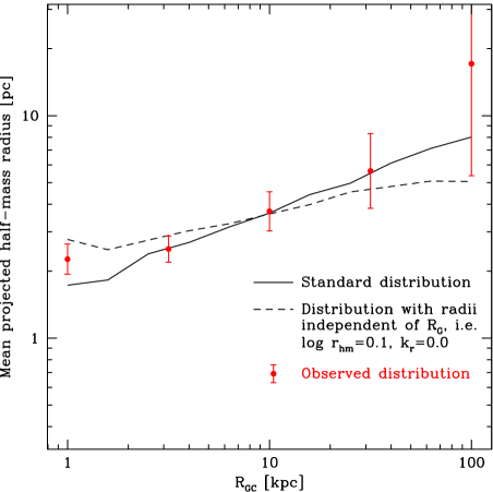
Figure 6: Mean projected half-mass radii of the simulated clusters as a function Galactocentric distance compared to the observed distribution of Milky Way clusters in runs with gas expulsion. The standard distribution (solid line) which has initial cluster radii increasing with Galactocentric distance fits the observed distribution very well. A distribution with constant $\log r_{hm}/\mbox{pc}=0.1$ independent of Galactocentric distance (dashed line) also provides a good fit since a larger fraction of clusters with large radii survive in the outer parts, leading to an increase of the average cluster radius with Galactocentric distance. The observed increase of half-mass radius with Galactocentric distance could therefore be either primordial or due to the dynamical evolution.

In our standard model, the average cluster radii were initially increasing with Galactocentric distance according to $<\!\log r_{h}/\mbox{pc}\!>=-0.1+0.2\cdot\log R_{G}/\mbox{kpc}$. Due to gas expulsion, the clusters expand on average by a factor of 2 to 3 and subsequent stellar evolution mass loss leads to another adiabatic expansion by 30%. It can be seen that the resulting distribution of cluster radii is in very good agreement with the observed distribution for both inner ($R_{G}<8$ kpc) and outer clusters. Our adopted slope of $k_{r}=0.2$ leads to a final slope which is close to the value of 0.42 found by Mackey & van den Bergh (2005) in their analysis of the present-day Galactic globular cluster system. In this scenario, the half-mass radii of inner globular clusters in the gas embedded phase are close to the half-mass radii of young, embedded clusters in the Galactic disc, $r_{h}\approx 0.5$ pc (Lada & Lada, 2003).

A distribution with constant $\log r_{hm}/\mbox{pc}=0.1$ independent of Galactocentric distance also provides an acceptable fit, since a larger fraction of clusters with large radii survive in the outer parts, leading to an increase of the average cluster radius with Galactocentric distance. The observed increase of half-mass radius with Galactocentric distance could therefore be either primordial or due to gas expulsion and later dynamical evolution.

Figure 7: Final mass distribution as a function of Galactocentric distance of the simulated clusters compared to the observed distribution of all Milky Way clusters in runs with gas expulsion. Distributions with an initial power-law profile with exponent $\alpha_{G}=4.5$ (solid and dashed lines) fit the observed distribution very well. Distributions with an initial power-law index $\alpha_{G}=3.5$ (long-dashed and dotted), which is similar to the present-day observed profile, lead to final profiles which are too flat. The Galactic globular cluster system must therefore have started with a more concentrated distribution then what is observed now. In addition, the orbital anisotropy seems to have only a small influence on the final density profile.

Fig. 7 finally depicts the mass density profile of the globular cluster system as a function of Galactocentric distance. Gas-embedded density distributions starting from $\alpha_{G}=4.5$ power-law distributions lead to final distributions which are in good agreement with the observations (solid and dashed lines). The reason is the efficient depletion of clusters at small Galactocentric distances, which flattens the overall profile. The final distribution is nearly independent of the initial amount of anisotropy. If clusters start with a density profile with power-law index $\alpha_{G}=3.5$, similar to what is observed now, the final profile becomes too strongly flattened and does not fit the observed profile. The Galactic globular cluster system should therefore have started more centrally concentrated than as we observe today and many clusters were lost from it in the inner parts of the Galaxy.

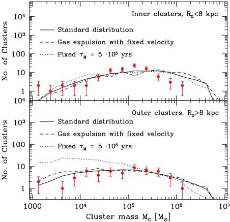
Figure 8: Mass distribution of star clusters after a Hubble time for the standard model (solid lines), a model which assumes gas outflow with a velocity of $v_{s}=10$ km/s (dashed lines), and a model which assumes a fixed gas expulsion timescale of $\tau_{M}=5\cdot 10^{5}$ yrs (dotted lines). In all cases, fewer low-mass clusters survive compared to a model without gas expulsion (see Fig. 1). The final distributions are in agreement with the observations for the standard case and models with fixed outflow velocity. Models with fixed expulsion timescale predict a factor 10 too many low-mass clusters at large Galactocentric radii.

3.4 Dependence of results on the assumed model for gas expulsion

In order to test how these results depend on the assumed model for gas expulsion, we also tried two additional models for gas expulsion. In one model, we follow Kroupa & Boily (2002) and assume that the gas leaves star clusters with the sound speed of the interstellar medium, $v_{s}\approx 10$ km/s, and set the gas expulsion timescale equal to $\tau_{M}=r_{h}/v_{s}$ for all clusters. Since observations show that star clusters are free of their primordial gas after one Myr (Kroupa, 2005), we set $\tau_{M}=0.5$ Myrs in the third model.

Fig. 8 depicts the resulting mass function of star clusters after a Hubble time for all three models. It can be seen that the distribution of star clusters inside $R_{G}=8\mbox{kpc}$ is always in good agreement to the observed distribution and does not depend much on the assumed model for gas expulsion. The reason is the strong dissolution of star clusters which causes most low-mass clusters to have come from relatively high-mass, $M_{C}\approx 10^{5}$ M_⊙, progenitors. Since most of these survive gas expulsion, the final distribution is nearly independent of the assumed model for gas expulsion.

In the outer parts, a factor of 5 to 10 too many low-mass clusters survive in case of gas expulsion with fixed gas expulsion timescale. But even in this case there is a strong depletion of star clusters by about a factor 100 compared to the initial number of clusters, so small changes in the assumed cluster dissolution model might bring the expected distribution into agreement with the observations. The model with constant outflow velocity on the other hand is in good agreement with the observations. A range of gas expulsion models might therefore be able to turn an initial power-law mass function for the gas embedded clusters into a Gaussian for the present-day clusters.

3.5 The origin of the Galactic halo stars

Using our best-fitting models, we now turn to the connection between the Galactic halo stars and globular clusters. Baumgardt (1998) and Kroupa & Boily (2002) suggested that if stars always form in clusters ranging from the lowest to the highest masses, then infant mortality and cluster dissolution will naturally produce field populations derived from the disrupted low to intermediate-mass clusters. A common origin of field halo stars and stars in globular clusters is also indicated by similarities in their heavy element abundances (Sneden, 2005). In our standard model, only 5.2% of all stars initially in star clusters end up in present-day globular clusters. The majority of stars is lost from clusters either due to gas expulsion or the later dynamical evolution and dissolution of the clusters. Our simulations show that both processes contribute with approximately equal strength to stars lost from clusters.

According to Freeman & Bland-Hawthorn (2002), the total mass of the stellar halo is $\sim 10^{9}$ M_⊙. The total mass of metal-poor globular clusters with [Fe/H]$<-0.8$, which are believed to be connected to the stellar halo (Zinn, 1993), is $2\cdot 10^{7}$ M_⊙. The initial mass in star clusters with mass $M_{C}>10^{3}$ M_⊙ is therefore about half the stellar halo mass. Taking into account clusters with masses 10 M${}_{\odot}<M_{C}<10^{3}$ M_⊙ would increase this estimate by another 50%. It hence seems possible that the entire stellar halo formed from dissolved star clusters, confirming the notion of Baumgardt (1998) and Kroupa & Boily (2002), see also Parmentier & Gilmore (2007).

The density of field halo stars can be well fitted by a power-law with exponent $\alpha=-3.55\pm 0.13$ between $8<R_{G}<35$ kpc (Chiba & Beers, 2000). If the field halo stars come from dissolved, low-metallicity clusters, these clusters must have followed the same initial density profile. Fig. 9 compares the density profile of halo clusters with [Fe/H]$<0.8$ with the predicted profiles, given different initial power-law distributions. It can be seen that density distributions starting from steep power-laws generally provide the best fit to the observations. However, density profiles starting with flatter initial distributions in the range $3.5<\alpha_{G}<3.8$ also provide acceptable fits to the density of halo globular clusters between 5 kpc $<R_{G}<20$ kpc. It therefore seems very likely that field halo stars come from dissolved globular clusters.

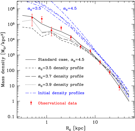
Figure 9: Observed mass density distribution of halo clusters with $\mbox{[Fe/H]}<-0.8$ as a function of Galactocentric distance compared to the final distributions for clusters starting from different initial density profiles. The distribution starting with an initial power-law profile with exponent $\alpha_{G}=4.5$ (solid line) for the gas embedded clusters fits the observed distribution very well. However, distributions with initial power-law indices in the range $3.5<\alpha_{G}<3.9$, which are in better agreement with the observed distribution of halo stars, also provide acceptable fits to the observed cluster distribution at radii between $5<R_{G}<20$ kpc. It therefore seems possible that halo stars and globular clusters share a common origin.

The field halo stars have a radially elongated velocity ellipsoid with components $(\sigma_{u},\sigma_{V},\sigma_{W})=(141\pm 11,106\pm 9,94\pm 8)$ km/s (Chiba & Beers, 2000), corresponding to $\beta_{v}=0.5$. Due to the efficient destruction of star clusters on radial orbits, the anisotropy of the globular cluster system is decreasing with time. If field halo stars come from dissolved star clusters, and if star clusters start with a radial anisotropic velocity dispersion with $\beta_{v}=0.5$, we predict a nearly isotropic distribution with $\beta_{v}=0.01$ for the surviving star clusters after a Hubble time. The velocity dispersion of Galactic globular clusters can be tested if accurate proper motions become available, which should be possible with future astrometric space missions like e.g. GAIA.

4 Conclusions

We have followed the evolution of the Galactic globular cluster system under the influence of various dissolution mechanisms, taking into account the effect of residual gas expulsion. We assumed that gas embedded star clusters start with power-law mass functions, similar to what is observed for the Galactic open clusters and young, massive star clusters in interacting galaxies. The dissolution of the clusters was then studied under the combined influence of residual gas expulsion, stellar mass-loss, two-body relaxation and an external tidal field. The influence of gas expulsion was modeled by using a large set of $N$-body models computed by Baumgardt & Kroupa (2007).

We find that residual gas expulsion is the main dissolution mechanism for star clusters, destroying about 95% of them within a few 10s of Myr. It is possible to turn an initial power-law mass function for gas embedded clusters into a present-day log-normal one, because clusters with masses less than $10^{5}M_{\odot}$ lose their residual gas on a timescale shorter than their crossing times, as shown by our feedback analysis. In this case, the final mass function of globular clusters is established mainly by the gas expulsion and therefore nearly independent of the strength of the external tidal field, providing a natural explanation for the observed universality of the peak of the globular cluster mass function within a galaxy and among different galaxies. Observational evidence for such rapid gas expulsion is discussed by Kroupa (2005). In such a case, a characteristic mass-scale of $\approx 10^{5}\mbox{M}_{\odot}$, as was suggested by Fall & Rees (1985), does not exist for globular clusters, and they instead form from a feature-less power-law mass function, as present epoch clusters are observed to do (Larsen, 2004).

Our best-fitting model for the distribution of Galactic globular clusters has the following parameters: The slope of the mass function of gas embedded clusters is $\beta=2.0$, close to what is observed for young star clusters in starburst galaxies or the open clusters in the Milky Way (Whitmore & Schweizer, 1995; Whitmore et al., 1999; Larsen, 2002; Fuente Marcos & Fuente Marcos, 2004; Gieles et al., 2006). This slope is also similar to that found for the mass function of molecular-cloud cores (Solomon et al., 1987; Engargiola et al., 2003; Rosolowsky, 2005). Slightly steeper mass functions with $\beta=2.3$ are also allowed, but flatter mass distributions of gas embedded clusters with $\beta\approx 1.5$ lead to final distributions which are inconsistent with the observed mass distribution of Milky Way globular clusters.

The current distribution of half-mass radii of globular clusters can be fitted with an initial log-normal distribution with mean $\log(r_{h}/\mbox{pc})=-0.1+0.2\log(R_{G}/\mbox{kpc})$ and dispersion $\sigma_{R}=0.2$, or a distribution with $\log(r_{h}/\mbox{pc})=0.1$ and dispersion $\sigma_{R}=0.2$ independent of Galactocentric distance. Globular clusters should therefore have started with half-mass radii several times smaller than as we see them today. The observed dependence of mean half-mass radius on Galactocentric distance (van den Bergh, 1994; Mackey & van den Bergh, 2005) is either primordial, pointing to differences in the formation of the clusters, or coming from the gas expulsion and the higher survival probability of extended star clusters at larger Galactocentric distances. In terms of a unifying cluster formation theory, this latter solution appears more attractive.

The present-day radial density distribution of clusters can be well fitted by an initial power-law density distribution with slope $\alpha_{G}=4.5$ of the gas-embedded clusters. Low-metallicity globular clusters with [Fe/H]$<-0.8$ could also have started from flatter density distributions with slopes $\alpha_{G}$ as low as $\alpha_{G}=3.5$, which is similar to the density distribution of halo field stars (Chiba & Beers, 2000).

It seems possible that all halo field stars originate from dissolved star clusters. In this case halo field stars come mostly from low-mass clusters ($M_{C}<10^{4}$ M_⊙), which quickly dissolve due to either residual gas expulsion or dynamical cluster evolution. In addition, gas lost by stellar winds from stars in low-mass clusters is likely to escape due to the low escape speeds. Chemical enrichment due to massive stars within the same cluster is therefore unlikely to have taken place and, if the material out of which the clusters formed was well mixed, could explain why no abundance anomalies are seen in halo stars (Gratton et al., 2000, 2004).

Stars in globular clusters on the other hand could have been enriched by material lost from more massive stars within the same cluster, especially if the winds from these stars are slow as has been recently suggested by Decressin et al. (2007). Slow winds would also be inefficient in dispersing gas clouds and therefore increase the gas expulsion time scale $\tau_{M}$ and hence the survival chances of star clusters. In order to explain the near homogeneity of heavy elements in globular clusters, ejecta from supernova explosions should not be retained, hence the clusters would either have to be already gas free by the time the supernova explosions go off or the gas was driven out by these explosions. Hence, most of the enrichment of stars in globular clusters should take place within a few Myr, pointing to heavy main-sequence stars with masses between $10-120$ M_⊙ as the polluters. This point has recently been stressed also by Decressin et al. (2007). Heavy main-sequence stars as sources for metal-enrichment also have the advantage that a standard stellar IMF would be sufficient and one does not have to invoke an unusual flat IMF as in case of pollution by AGB stars (D’Antona & Caloi, 2004; Prantzos & Charbonnel, 2006).

Due to the efficient destruction of star clusters on radial orbits, the velocity anisotropy of the globular cluster system is decreasing with time. If field halo stars come from dissolved star clusters, and if star clusters start with a radial anisotropic velocity dispersion with $\beta_{v}=0.5$ similar to what is seen for field halo stars (Chiba & Beers, 2000), we predict an isotropic distribution for the surviving star clusters after a Hubble time.

References

- Bastian & Goodwin (2006) Bastian, N., Goodwin, S., 2006, MNRAS, 369, 9
- Baumgardt (1998) Baumgardt, H., 1998, A&A, 330, 480
- Baumgardt (2001) Baumgardt, H., 2001, MNRAS, 325, 1323
- Baumgardt, Hut & Heggie (2002) Baumgardt, H., Hut, P., Heggie, D. C., 2002, MNRAS, 336, 1069
- Baumgardt & Makino (2003) Baumgardt, H., Makino, J., 2003, MNRAS, 340, 227
- Baumgardt & Kroupa (2007) Baumgardt, H., Kroupa, P., 2007, MNRAS 380, 1589
- Binney & Tremaine (1987) Binney, J., Tremaine, S., 1987, Galactic Dynamics, Princeton Univ. Press, Princeton
- Boily & Kroupa (2003a) Boily, C. M., Kroupa, P., 2003a, MNRAS, 338, 665
- Boily & Kroupa (2003b) Boily, C. M., Kroupa, P., 2003b, MNRAS, 338, 673
- Boutloukos & Lamers (2003) Boutloukos, S. G., Lamers, H. J. G. L. M., 2003, MNRAS, 338, 717
- Chaboyer et al. (1998) Chaboyer, B., Demarque, P., Kernan, P. J., Krauss, L. M., 1998, ApJ, 494, 96
- Chandar, Fall & Whitmore (2006) Chandar, R., Fall, S. M., Whitmore, B. C., 2006, ApJ, 650, L111
- Chiba & Beers (2000) Chiba, M., Beers, T. C., 2000, AJ, 119, 2843
- Dabringhausen et al. (2008) Dabringhausen, J., Kroupa, P., Hilker, M., 2008, MNRAS in prep.
- D’Antona & Caloi (2004) D’Antona, F., Caloi, V., 2004, ApJ, 611, 871
- de Grijs et al. (2003) de Grijs, R., et al., 2003, MNRAS, 343, 1285
- Decressin et al. (2007) Decressin, T., Meynet, G., Charbonnel, C., Prantzos, N., Ekström, S., 2007, A&A, 464, 1029
- Decressin et al. (2007) Decressin, T., Charbonnel, C., Meynet, G., 2007, A&A in press, astro-ph/0709.4160v1
- Engargiola et al. (2003) Engargiola, G., Plambeck, R. L., Rosolowsky, E., Blitz, L., 2003, ApJS, 149, 343
- Evstigneeva et al. (2007) Evstigneeva, E. A., Gregg, M. D., Drinkwater, M. J., Hilker, M., 2007, AJ in press, astro-ph/0612483v1
- Fall & Zhang (2001) Fall, S. M., Zhang, Q., 2001, ApJ, 561, 751
- Fall & Rees (1985) Fall, S. M., Rees, M. J., 1985, ApJ, 298, 18
- Freeman & Bland-Hawthorn (2002) Freeman, K., Bland-Hawthorn, J., 2002, ARA&A, 40, 487
- Freyer, Hensler & Yorke (2006) Freyer, T., Hensler, G., Yorke, H. W., 2006, ApJ, 638, 262
- Freyer, Hensler & Yorke (2003) Freyer, T., Hensler, G., Yorke, H. W., 2003, ApJ, 594, 888
- Gieles et al. (2006) Gieles, M., et al., 2006, A&A, 450, 129
- Gieles, Lamers & Portegies Zwart (2006) Gieles, M., Lamers, H., Portegies Zwart, S., 2006, ApJ submitted, astro-ph/0706.1202
- Gnedin & Ostriker (1996) Gnedin, O. Y., Ostriker, J. P., 1996, ApJ, 474, 223
- Goodwin & Bastian (2006) Goodwin, S., Bastian, N., 2006, MNRAS, 373, 752
- Gratton et al. (2000) Gratton, R. G., Sneden, C., Carretta, E., Bragaglia, A., 2000, A&A, 354, 169
- Gratton et al. (2003) Gratton, R. G., et al., 2003, A&A, 408, 529
- Gratton et al. (2004) Gratton, R. G., Sneden, C., Carretta, E., 2004, ARA&A, 42, 385
- Fuente Marcos & Fuente Marcos (2004) de la Fuente Marcos, R., de la Fuente Marcos, C., 2004, New Astronomy, 9, 475
- Harris (1991) Harris, W. E., 1991, ARA&A, 29, 543
- Harris (1996) Harris, W. E., 1996, AJ, 112, 1487
- Harris, Harris & McLaughlin (1998) Harris, W. E., Harris, G. L. H., McLaughlin, D. E., 1998, AJ, 115, 1801
- Hilker & Richtler (2000) Hilker, M., Richtler, T., 2000, A&A, 362, 895
- Hills (1980) Hills, J. G., 1980, ApJ, 235, 986
- Innanen, Harris & Webbink (1983) Innanen, K. A., Harris, W. E., Webbink, R. F., 1983, ApJ, 88, 338
- Jórdan et al. (2006) Jórdan, A., et al., 2006, ApJ, 651, L25
- Kavelaars & Hanes (1997) Kavelaars, J. J., Hanes, D. A., 1997, MNRAS, 285, 31
- Kroupa (2000) Kroupa, P., 2000, New Astronomy 4, 615
- Kroupa (2001) Kroupa, P., 2001, MNRAS 322, 231
- Kroupa (2002) Kroupa, P., 2002, MNRAS 330, 707
- Kroupa (2005) Kroupa, P., 2005, The Fundamental Building Blocks of Galaxies, in Proceedings of the Gaia Symposium ”The Three-Dimensional Universe with Gaia”, Turon, C., O’Flaherty, K.S., Perryman, M.A.C., eds., p. 629, astro-ph/0412069
- Kroupa, Aarseth & Hurley (2001) Kroupa, P., Aarseth, S., Hurley, J., 2001, MNRAS, 321, 707
- Kroupa & Boily (2002) Kroupa, P., Boily, C. M., 2002, MNRAS 336, 1188
- Kroupa, Petr & McCaughrean (1999) Kroupa, P., Petr, M. G., McCaughrean, M. J., 1999, New Astronomy 4, 495
- Kroeger et al. (2007) Kröger D., Freyer T., Hensler, G., Yorke, H. W., 2007, preprint
- Kundu & Whitmore (2001a) Kundu, A., Whitmore, B. C., 2001, AJ, 121, 2950
- Kundu & Whitmore (2001b) Kundu, A., Whitmore, B. C., 2001, AJ, 122, 1251
- Lada & Lada (2003) Lada, C. J., Lada, E. A., 2003, ARAA, 41, 57
- Lamers, Gieles & Portegies Zwart (2005) Lamers, H. J. G. L. M., Gieles, M., Portegies Zwart, S., 2005, A&A, 429, 173
- Larsen (2002) Larsen, S. S., 2002, AJ, 124, 1393
- Larsen (2004) Larsen, S. S., 2004, A&A, 416, 537
- Mackey & van den Bergh (2005) Mackey, A. D., van den Bergh, S., 2005, MNRAS, 360, 631
- McLaughlin & Fall (2007) McLaughlin, D. E., Fall, S. M., 2007, ApJ submitted, arXiv:0704.0080v1
- Meylan et al. (2001) Meylan, G., et al., 2001, AJ, 122, 830
- Nantais et al. (2006) Nantais, J. B., et al., 2006, AJ, 131, 1416
- Okazaki & Tosa (1995) Okazaki, T., Tosa, M., 1995, MNRAS, 274, 480
- Ostriker, Spitzer, & Chevalier (1972) Ostriker, J. P., Spitzer, L. Jr., Chevalier, R. A., 1972, ApJ, 176, L52
- Parmentier & Gilmore (2005) Parmentier, G., Gilmore, G., 2005, MNRAS, 363, 326
- Parmentier & Gilmore (2007) Parmentier, G., Gilmore, G., 2007, MNRAS, 377, 352
- Parmentier et al. (2008) Parmentier, G. et al., 2008, MNRAS in preparation
- Pellerin et al. (2006) Pellerin, A., Meyer, M., Harris, J., Calzetti, D., 2006, in Mass Loss from Stars and the Evolution of Stellar Clusters Conference, eds. A. de Kater, L. Smith and R. Waters, ASO Conf. Ser., astro-ph/0610798
- Piotto et al. (2005) Piotto, G., et al., 2005, ApJ, 621, 777
- Prantzos & Charbonnel (2006) Prantzos, N., Charbonnel, C., 2006, A&A, 458, 135
- Rosolowsky (2005) Rosolowsky, E., 2005, PASP, 117, 1403
- Secker (1992) Secker, J., 1992, AJ, 104, 1472
- Sneden (2005) Sneden, C., 2005, in From Lithium to Uranium: Elemental Tracers of Early Cosmic Evolution Conference, eds. V. Hill, P. Francois, F. Primas, IAU Symp. 228, p. 337
- Solomon et al. (1987) Solomon, P. M., Rivolo, A. R., Barrett, J., Yahil, A., 1987, ApJ, 319, 730
- Spitzer (1969) Spitzer, L. Jr., 1969, ApJ, 158, 139
- Tamura et al. (2006) Tamura, N., et al., 2006, MNRAS, 373, 588
- Tremaine, Ostriker & Spitzer (1975) Tremaine, S., Ostriker, J. P., Spitzer, L. Jr., 1975, ApJ, 196, 407
- VandenBerg et al. (2002) VandenBerg, D. A., Richard, O., Michaud, G., Richer, J., 2002, ApJ, 571, 487
- van den Bergh (2006) van den Bergh, S., 2006, AJ, 131, 304
- van den Bergh (1994) van den Bergh, S., 1994, AJ, 108, 2145
- Verschueren (1990) Verschueren, W., 1990, A&A, 234, 156
- Vesperini (1998) Vesperini, E., 1998, MNRAS, 299, 1019
- Vesperini (2000) Vesperini, E., 2000, MNRAS, 318, 841
- Vesperini (2001) Vesperini, E., 2001, MNRAS, 322, 247
- Vesperini & Heggie (1997) Vesperini, E., Heggie, D. C., 1997, MNRAS, 289, 898
- Vesperini et al. (2003) Vesperini, E., Zepf, S. E., Kundu, A., Ashman, K. M., 2003, ApJ, 593, 760
- Weidner et al. (2004) Weidner, C., Kroupa, P., Larsen, S. S., 2004, MNRAS, 350, 1503
- Weidner et al. (2007) Weidner, C., Kroupa, P., Nürnberger, D. E. A., Sterzik, M. F., 2007, MNRAS in press, astro-ph/0702001
- Whitmore & Schweizer (1995) Whitmore, B. C., Schweizer, F., 1995, AJ, 109, 960
- Whitmore et al. (1999) Whitmore, B. C., et al., 1999, AJ, 118, 1551
- Whitmore et al. (2002) Whitmore, B. C., Schweizer, F., Kundu, A., Miller, B. W., 2002, AJ, 124, 147
- Fall & Zhang (1999) Zhang, Q., Fall, S. M., 1999, ApJ, 527, L81
- Zinn (1993) Zinn, R., 1993, in The globular clusters-galaxy connection, ASP Conf. Ser. 48, G. H. Smith and J. P. Brodie eds., p. 38