Lines of Curvature on Surfaces, Historical Comments and Recent Developments

Abstract.

This survey starts with the historical landmarks leading to the study of principal configurations on surfaces, their structural stability and further generalizations. Here it is pointed out that in the work of Monge, 1796, are found elements of the qualitative theory of differential equations (QTDE), founded by Poincaré in 1881. Here are also outlined a number of recent results developed after the assimilation into the subject of concepts and problems from the QTDE and Dynamical Systems, such as Structural Stability, Bifurcations and Genericity, among others, as well as extensions to higher dimensions. References to original works are given and open problems are proposed at the end of some sections.

1. Introduction

The book on differential geometry of D. Struik [78], remarkable for its historical notes, contains key references to the classical works on principal curvature lines and their umbilic singularities due to L. Euler [8], G. Monge [60], C. Dupin [7], G. Darboux [6] and A. Gullstrand [38], among others (see [77] and, for additional references, also [50]). These papers —notably that of Monge, complemented with Dupin’s— can be connected with aspects of the qualitative theory of differential equations (QTDE for short) initiated by H. Poincaré [65] and consolidated with the study of the structural stability and genericity of differential equations in the plane and on surfaces, which was made systematic from $1937$ to $1962$ due to the seminal works of Andronov Pontrjagin and Peixoto (see [1] and [63]).

This survey paper discusses the historical sources for the work on the structural stability of principal curvature lines and umbilic points, developed by C. Gutierrez and J. Sotomayor [43, 44, 48]. Also it addresses other kinds of geometric foliations studied by R. Garcia and J. Sotomayor [27, 29, 33]. See also the papers devoted to other differential equations of classical geometry: the asymptotic lines [18, 28], and the arithmetic, geometric and harmonic mean curvature lines [30, 31, 32, 33].

In the historical comments posted in [76] it is pointed out that in the work of Monge, [60], are found elements of the QTDE, founded by Poincaré in [65].

The present paper contains a reformulation of the essential historical aspects of [74, 75]. Following the thread of Structural Stability and the QTDE it discusses pertinent extensions and updates references. At the end of some sections related open problems are proposed and commented.

Extensions of the results outlined in section 2.3 to surfaces with generic critical points, algebraic surfaces, surfaces and $3$ dimensional manifolds in ${\mathbb{R}}^{4}$ have been achieved recently (see, for example, [16, 18, 22, 27, 28, 29, 35, 36, 58]). An account of these recent developments will be given here.

2. Historical Landmarks

2.1. The Landmarks before Poincaré: Euler, Monge and Dupin

Leonhard Euler (1707-1783) [8], founded the curvature theory of surfaces. He defined the normal curvature $k_{n}(p,L)$ on an oriented surface S in a tangent direction $L$ at a point $p$ as the curvature, at $p$, of the planar curve of intersection of the surface with the plane generated by the line $L$ and the positive unit normal $N$ to the surface at $p$. The principal curvatures at $p$ are the extremal values of $k_{n}(p,L)$ when $L$ ranges over the tangent directions through $p$. Thus, $k_{1}(p)=k_{n}(p,L_{1})$ is the minimal and $k_{2}(p)=k_{n}(p,L_{2})$ is the maximal normal curvatures, attained along the principal directions: $L_{1}(p)$, the minimal, and $L_{2}(p)$, the maximal (see Fig. 1).

Euler’s formula expresses the normal curvature $k_{n}(\theta)$ along a direction making angle $\theta$ with the minimal principal direction $L_{1}$ as $k_{n}(\theta)=k_{1}\cos^{2}\theta+k_{2}\sin^{2}\theta$.

Euler, however, seems to have not considered the integral curves of the principal line fields $L_{i}:p\to L_{i}(p),\,i\,=1,\,2,\,$ and overlooked the role of the umbilic points at which the principal curvatures coincide and the line fields are undefined.

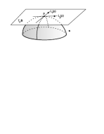
Figure 1. Principal Directions.

Gaspard Monge (1746-1818) found the family of integral curves of the principal line fields $L_{i},i\,=1,\,2,\,$ for the case of the triaxial ellipsoid

$$\frac{x^{2}}{a^{2}}+\frac{y^{2}}{b^{2}}+\frac{z^{2}}{c^{2}}-1=0,\,\,\,a>b>c>0.$$

In doing this, by direct integration of the differential equations of the principal curvature lines, circa 1779, Monge was led to the first example of a foliation with singularities on a surface which (from now on) will be called the principal configuration of an oriented surface. The singularities consist on the umbilic points, mathematical term he coined to designate those at which the principal curvatures coincide and the line fields are undefined.

The Ellipsoid, endowed with its principal configuration, will be called Monge’s Ellipsoid (see Fig. 2).

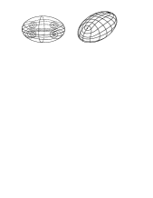
Figure 2. Monge’s Ellipsoid, two perspectives.

The motivation found in Monge’s paper [60] is a complex interaction of esthetic and practical considerations and of the explicit desire to apply the results of his mathematical research to real world problems. The principal configuration on the triaxial ellipsoid appears in Monge’s proposal for the dome of the Legislative Palace for the government of the French Revolution, to be built over an elliptical terrain. The lines of curvature are the guiding curves for the workers to put the stones. The umbilic points, from which were to hang the candle lights, would also be the reference points below which to put the podiums for the speakers.

Commenting Monge’s work under the perspective of the QTDE The ellipsoid depicted in Fig. 2 contains some of the typical features of the qualitative theory of differential equations discussed briefly in a) to d) below:

a) Singular Points and Separatrices. The umbilic points play the role of singular points for the principal foliations, each of them has one separatrix for each principal foliation. This separatrix produces a connection with another umbilic point of the same type, for which it is also a separatrix, in fact an umbilic separatrix connection.

b) Cycles. The configuration has principal cycles. In fact, all the principal lines, with the exception of the four umbilic connections, are periodic. The cycles fill a cylinder or annulus, for each foliation. This pattern is common to all classical examples, where no surface exhibiting an isolated cycle was known. This fact seems to be derived from the symmetry of the surfaces considered, or from the integrability that is present in the application of Dupin’s Theorem for triply orthogonal families of surfaces.

As was shown in [43], these configurations are exceptional; the generic principal cycle for a smooth surface is a hyperbolic limit cycle (see below).

c) Structural Stability (relative to quadric surfaces). The principal configuration remains qualitatively unchanged under small perturbations on the coefficients of the quadratic polynomial that defines the surface.

d) Bifurcations. The drastic changes in the principal configuration exhibited by the transitions from a sphere, to an ellipsoid of revolution and to a triaxial ellipsoid (as in Fig. 2), which after a very small perturbation, is a simple form of a bifurcation phenomenon.

Charles Dupin (1784-1873) considered the surfaces that belong to triply orthogonal surfaces, thus extending considerably those whose principal configurations can be found by integration. Monge’s Ellipsoid belongs to the family of homofocal quadrics (see [78] and Fig. 3).

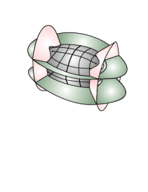
Figure 3. Dupin’s Theorem.

The conjunction of Monge’s analysis and Dupin extension provides the first global theory of integrable principal configurations, which for quadric surfaces gives those which are also principally structurally stable under small perturbations of the coefficients of their quadratic defining equations.

Theorem 1.

[74] In the space of oriented quadrics, identified with the nine-dimensional sphere, those having principal structurally stable configurations are open and dense.

Historical Thesis in [76]. The global study of lines of principal curvature leading to Monge’s Ellipsoid, which is analogous of the phase portrait of a differential equation, contains elements of Poincaré’s QTDE, 85 years earlier.

This connection seems to have been overlooked by Monge’s scientific historian René Taton (1915-2004) in his remarkable book [79].

2.2. Poincaré and Darboux

The exponential role played by Henri Poincaré (1854-1912) for the QTDE as well as for other branches of mathematics is well known and has been discussed and analyzed in several places (see for instance [3] and [64]).

Here we are concerned with his Mémoires [65], where he laid the foundations of the QTDE. In this work Poincaré determined the form of the solutions of planar analytic differential equations near their foci, nodes and saddles. He also studied properties of the solutions around cycles and, in the case of polynomial differential equations, also the behavior at infinity. Gaston Darboux (1842-1917) determined the structure of the lines of principal curvature near a generic umbilic point. In his note [6], Darboux uses the theory of singularities of Poincaré. In fact, the Darbouxian umbilics are those whose resolution by blowing up reduce only to saddles and nodes (see Figs. 4 and 5).

Figure 4. Darbouxian Umbilics.

Let $\mathbf{p}_{0}\in\mathbf{S}$ be an umbilic point. Consider a chart $(u,v):(\mathbf{S},\mathbf{p}_{0})\to({\mathbb{R}}^{2},\mathbf{0})$ around it, on which the surface has the form of the graph of a function such as

$$\frac{k}{2}(u^{2}+v^{2})+\frac{a}{6}u^{3}+\frac{b}{2}uv^{2}+\frac{c}{6}v^{3}+O[(u^{2}+v^{2})^{2}].$$

This is achieved by projecting $\mathbf{S}$ onto $T_{\mathbf{p}_{0}}\mathbf{S}$ along $N(\mathbf{p}_{0})$ and choosing there an orthonormal chart $(u,v)$ on which the coefficient of the cubic term $u^{2}v$ vanishes.

An umbilic point is called Darbouxian if, in the above expression, the following 2 conditions T) and D) hold:

T) $b(b-a)\neq 0$,

D) either

D₁: $a/b>(c/2b)^{2}+2$,

D₂: $(c/2b)^{2}+2>a/b>1$, $a\neq 2b$,

D₃: $a/b<1.$

The corroboration of the pictures in Fig. 4, which illustrate the principal configurations near Darbouxian umbilics, has been given in [43, 48]; see also [4] and Fig. 5 for the Lie-Cartan resolution of a Darbouxian umbilic.

The subscripts refer to the number of umbilic separatrices, which are the curves, drawn with heavy lines, tending to the umbilic point and separating regions whose principal lines have different patterns of approach.

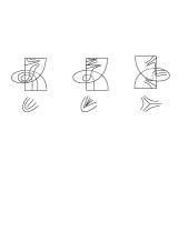
Figure 5. Lie-Cartan Resolution of Darbouxian Umbilics.

2.3. Principal Configurations on Smooth Surfaces in $\mathbb{R}^{3}$

After the seminal work of Andronov-Pontrjagin [1] on structural stability of differential equations in the plane and its extension to surfaces by Peixoto [63] and in view of the discussion on Monge’s Ellipsoid formulated above, an inquiry into the characterization of the oriented surfaces $\mathbf{S}$ whose principal configuration are structurally stable under small $C^{r}$ perturbations, for $r\geq 3$, seems unavoidable.

Call $\Sigma(a,b,c,d)$ the set of smooth compact oriented surfaces $\mathbf{S}$ which verify the following conditions.

a) All umbilic points are Darbouxian. b) All principal cycles are hyperbolic. This means that the corresponding return map is hyperbolic; that is, its derivative is different from 1. It has been shown in [43] that hyperbolicity of a principal cycle $\gamma$ is equivalent to the requirement that

$$\int_{\gamma}\frac{d\mathcal{H}}{\sqrt{\mathcal{H}^{2}-\mathcal{K}}}\neq 0,$$

where $\mathcal{H}=(k_{1}+k_{2})/2$ is the mean curvature and $\mathcal{K}=k_{1}k_{2}$ is the gaussian curvature.

c) The limit set of every principal line is contained in the set of umbilic points and principal cycles of $\mathbf{S}$.

The $\alpha$-(resp. $\omega$) limit set of an oriented principal line $\gamma$, defined on its maximal interval $\mathcal{I}=(w_{-},w_{+})$ where it is parametrized by arc length $s$, is the collection $\alpha(\gamma)$-(resp. $\omega(\gamma)$) of limit point sequences of the form $\gamma(s_{n})$, convergent in $\mathbf{S}$, with $s_{n}$ tending to the left (resp. right) extreme of $\mathcal{I}$. The limit set of $\gamma$ is the set $\Omega=\alpha(\gamma)\cup\omega(\gamma)$.

Examples of surfaces with non trivial recurrent principal lines, which violate condition c are given in [44, 48] for ellipsoidal and toroidal surfaces.

There are no examples of these situations in the classical geometry literature.

d) All umbilic separatrices are separatrices of a single umbilic point.

Separatrices which violate d are called umbilic connections; an example can be seen in the ellipsoid of Fig. 2.

To make precise the formulation of the next theorems, some topological notions must be defined.

A sequence $\mathbf{S}_{n}$ of surfaces converges in the $C^{r}$ sense to a surface $\mathbf{S}$ provided there is a sequence of real functions $f_{n}$ on $\mathbf{S}$, such that $\mathbf{S}_{n}=(I+f_{n}N)(\mathbf{S})$ and $f_{n}$ tends to $0$ in the $C^{r}$ sense; that is, for every chart $(u,v)$ with inverse parametrization $X$, $f_{n}\circ X$ converges to $0$, together with the partial derivatives of order $r$, uniformly on compact parts of the domain of $X$.

A set $\Sigma$ of surfaces is said to be open in the $C^{r}$ sense if every sequence $\mathbf{S}_{n}$ converging to $\mathbf{S}$ in $\Sigma$ in the $C^{r}$ sense is, for $n$ large enough, contained in $\Sigma$.

A set $\Sigma$ of surfaces is said to be dense in the $C^{r}$ sense if, for every surface $\mathbf{S}$, there is a sequence $\mathbf{S}_{n}$ in $\Sigma$ converging to $\mathbf{S}$ the $C^{r}$ sense.

A surface $\mathbf{S}$ is said to be $C^{r}$-principal structurally stable if for every sequence $\mathbf{S}_{n}$ converging to $\mathbf{S}$ in the $C^{r}$ sense, there is a sequence of homeomorphisms $H_{n}$ from $\mathbf{S}_{n}$ onto $\mathbf{S}$, which converges to the identity of $\mathbf{S}$, such that, for $n$ big enough, $H_{n}$ is a principal equivalence from $\mathbf{S}_{n}$ onto $\mathbf{S}$. That is, it maps $\mathbf{U}_{n}$, the umbilic set of $\mathbf{S}_{n}$, onto $\mathbf{U}$, the umbilic set of $\mathbf{S}$, and maps the lines of the principal foliations $\mathbf{F}_{i,n}$, of $\mathbf{S}_{n}$, onto those of $\mathbf{F}_{i}$, $i=1,2$, principal foliations for $\mathbf{S}$.

Theorem 2.

(Structural Stability of Principal Configurations [43, 48]) The set of surfaces $\Sigma(a,b,c,d)$ is open in the $C^{3}$ sense and each of its elements is $C^{3}$-principal structurally stable.

Theorem 3.

(Density of Principal Structurally Stable Surfaces, [44, 48]) The set $\Sigma(a,b,c,d)$ is dense in the $C^{2}$ sense.

To conclude this section two open problems are proposed.

Problem 1.

Raise from 2 to 3 the differentiability class in the density Theorem 3.

This remains among the most intractable questions in this subject, involving difficulties of Closing Lemma type, [66], which also permeate other differential equations of classical geometry, [33].

Problem 2.

Is it possible to have a smooth embedding of the Torus $\mathbb{T}^{2}$ into $\mathbb{R}^{3}$ with both maximal and minimal non-trivial recurrent principal curvature lines?

Examples with either maximal or minimal principal recurrences can be found in [44, 48].

3. Curvature Lines near Umbilic Points

The purpose of this section is to present the simplest qualitative changes –bifurcations– exhibited by the principal configurations under small perturbations of an immersion which violates the Darbouxian structural stability condition on umbilic points.

It will be presented the two codimension one umbilic points D${}^{1}_{2}$ and D${}^{1}_{2,3}$, illustrated in Fig. 6 and the four codimension two umbilic points D${}^{2}_{1}\,$, D${}^{2}_{2p}\,$, D${}^{2}_{3}\,$ and D${}^{2}_{2h}$, illustrated in Figs. 4 and 8.

The superscript stands for the codimension which is the minimal number of parameters on which depend the families of immersions exhibiting persistently the pattern. The subscripts stand for the number of separatrices approaching the umbilic. In the first case, this number is the same for both the minimal and maximal principal curvature foliations. In the second case, they are not equal and, in our notation, appear separated by a comma. The symbols $p$, for parabolic, and $h$, for hyperbolic, have been added to the subscripts above in order to distinguish types that are not discriminated only by the number of separatrices.

3.1. Preliminaries on Umbilic Points

The following assumptions will hold from now on.

Let $p_{0}$ be an umbilic point of an immersion $\alpha$ of an oriented surface $\mathbb{M}$ into $\mathbb{R}^{3}$, with a once for all fixed orientation. It will be assumed that $\alpha$ is of class $C^{k},\;k\geq\,6$. In a local Monge chart near $p_{0}$ and a positive adapted $3-$frame, $\alpha$ is given by $\alpha(u,v)=(u,v,h(u,v))$, where

$$h(u,v) =\frac{k}{2}(u^{2}+v^{2})+\frac{a}{6}u^{3}+\frac{b}{2}uv^{2}+\frac{c}{6}v^{3}+\frac{A}{24}u^{4}+\frac{B}{6}u^{3}v$$ (1)

$$+\frac{C}{4}u^{2}v^{2}+\frac{D}{6}uv^{3}+\frac{E}{24}v^{4}+\frac{a_{50}}{120}u^{5}+\frac{a_{41}}{24}u^{4}v$$

$$+\frac{a_{32}}{12}u^{3}v^{2}+\frac{a_{23}}{12}u^{2}v^{3}+\frac{a_{14}}{24}uv^{4}+\frac{a_{05}}{120}v^{5}+h.o.t$$

Notice that, without loss of generality, the term $u^{2}v$ has been eliminated from this expression by means of a rotation in the $(u,v)-$ frame.

According to [77] and [78], the differential equation of lines of curvature in terms of $I=Edu^{2}+2Fdudv+Gdv^{2}$ and $II=edu^{2}+2fdudv+gdv^{2}$ around $p_{0}$ is:

$$(Fg-Gf)dv^{2}+(Eg-Ge)dudv+(Ef-Fe)du^{2}=0.$$ (2)

Therefore the functions $L=Fg-Gf$, $M=Eg-Ge$ and $N=Ef-Fe$ are:

$$L =h_{u}h_{v}h_{vv}-(1+h_{v}^{2})h_{uv}$$

$$M =(1+h_{u}^{2})h_{vv}-(1+h_{v}^{2})h_{uu}$$

$$N =(1+h_{u}^{2})h_{uv}-h_{u}h_{v}h_{uu}.$$

Calculation gives

$$L =-bv-\frac{1}{2}Bu^{2}-(C-k^{3})uv-\frac{1}{2}Dv^{2}-\frac{a_{41}}{6}u^{3}$$ (3)

$$+\frac{1}{2}(4bk^{2}+k^{2}a-a_{32})u^{2}v+\frac{1}{2}(3k^{2}c-a_{23})uv^{2}-\frac{1}{6}(a_{14}+3bk^{2})v^{3}+h.o.t$$

$$M =(b-a)u+cv+\frac{1}{2}(C-A+2k^{3})u^{2}+(D-B)uv+\frac{1}{2}({E-C}-2k^{3})v^{2}$$

$$+\frac{1}{6}[6bk^{2}(a+b)+a_{32}-a_{50}]u^{3}+\frac{1}{2}(a_{23}+2ck^{2}-a_{41})u^{2}v$$

$$+\frac{1}{2}[a_{14}-a_{32}-2k^{2}(a+b)]uv^{2}+\frac{1}{6}(a_{05}-a_{23}-6ck^{2})v^{3}+h.o.t$$

$$N =bv+\frac{1}{2}Bu^{2}+(C-k^{3})uv+\frac{1}{2}Dv^{2}+\frac{1}{6}a_{41}u^{3}$$

$$+\frac{1}{2}(a_{32}-3ak^{2})u^{2}v+\frac{1}{2}(a_{23}-k^{2}c)uv^{2}+\frac{1}{6}(a_{14}-3bk^{2})v^{3}+h.o.t$$

3.2. Umbilic Points of Codimension One

A characterization of umbilic points of codimension one is the following theorem announced in [45] and proved in [20].

Theorem 4.

[20, 45] Let $p_{0}$ be an umbilic point and consider $\alpha(u,v)=(u,v,h(u,v))$ as in equation (1). Suppose the following conditions hold:

• $cb(b-a)\neq 0\,$ and either  $(\frac{c}{2b})^{2}-\frac{a}{b}+1=0\quad$ or  $a=2b.$

• $b=a\neq 0\quad\text{and}\quad\chi={cB}-({C-A}+2k^{3})b\neq 0.$

Then the behavior of lines of curvature near the umbilic point $p_{0}$ in cases D${}^{1}_{2}$ and D${}^{1}_{2,3}$, is as illustrated in Fig. 6.

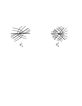
Figure 6. Principal curvature lines near the umbilic points D${}^{1}_{2}$, left, and D${}^{1}_{2,3}$, right, and their separatrices.

In Fig. 7 is illustrated the behavior of the Lie-Cartan resolution of the semi Darbouxian umbilic points.

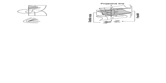
Figure 7. Lie-Cartan suspension D${}^{1}_{2}$, left, and D${}^{1}_{2,3}$, right.

Global effects, due to umbilic bifurcations, on these configurations such as the appearance and annihilation of principal cycles were studied in [20] and are outlined in section 7.

3.3. Umbilic Points of Codimension Two

The characterization of umbilic points of codimension two, generic in biparametric families of immersions, were established in [36] and will be reviewed in Theorem 5 below.

Theorem 5.

[36] Let $p_{0}$ be an umbilic point and $\alpha(u,v)=(u,v,h(u,v))$ as in equation (1).

• Case D${}^{2}_{1}$): If $\;\;c=0$   and   $a=2b\neq 0$,

  then the configuration of principal lines near $p_{0}$ is topologically equivalent to that of a Darbouxian D₁ umbilic point. See Fig. 4, left.

• If $a=b\neq 0$, $\chi=cB-b(C-A+2k^{3})=0$ and

  $\xi=12k^{2}b^{3}+(a_{32}-a_{50})b^{2}+(3B^{2}-3BD-ca_{41})b+3cB(C-k^{3})\neq 0,\,$

  then the principal configurations of lines of curvature fall into one of the two cases:

  • Case D${}^{2}_{2p}$: $\xi b<0$, which is topologically a D₂ umbilic and

  • Case D${}^{2}_{3}$:  $\xi b>0$, which is topologically a D₃ umbilic.

  See Fig. 4, center and right, respectively.

• Case D${}^{2}_{2h}$: If $a=b=0$ and $cB\neq 0$ or if $b=c=0$ and $aD\neq 0$, then the principal configuration near $p_{0}$ is as in Fig. 8.

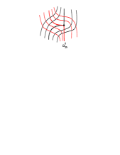
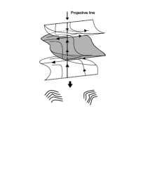
Figure 8. Lines of curvature near the umbilic point D${}^{2}_{2h}$, left, and associated Lie-Cartan suspension, right.

3.4. Umbilic Points of Immersions with Constant Mean Curvature

Let $(u,v)$ be isothermic coordinates in a neighborhood of an isolated umbilic point $p=0$ of an immersion $\alpha:\mathbb{M}^{2}\to\mathbb{R}^{3}$ with constant mean curvature ${\mathcal{H}}_{\alpha}$. In terms of $\phi=(e-g)/2-if$, and $w=u+iv$, the equation of principal lines is written as $\;Im(\phi(w)dw^{2})=0.$ See also [47] and [55]. The index of an isolated umbilical point with complex coordinate $w=0$ is equal to $-n/2$, where $n$ is the order of the zero of $\phi$ at $w=0$. There are $n+2$ rays $L_{0},\;L_{1},\ldots,L_{n+1}$ through $0\in T_{p}\mathbb{M}$, of which two consecutive rays make an angle of $2\pi/(n+2).$ Tangent at $p$ to each ray $L_{i}$, there is exactly one maximal principal line $S_{i}$ of ${\mathcal{F}}_{2}(\alpha)$ which approaches $p$. Two consecutive lines $S_{i}$, $S_{i+1}$, $i=0,1,2,\ldots,n+1$ $(S_{n+2}=S_{0})$, bound a hyperbolic sector of ${\mathcal{F}}_{2}(\alpha)$. The angular sectors bounded by $L_{i}$ and $L_{i+1}$ are bisected by rays $l_{i}$ , $i=0,1,\ldots,n+1$, which play for ${\mathcal{F}}_{1}(\alpha)$ the same role as $L_{i}$ for ${\mathcal{F}}_{2}(\alpha)$. See Fig. 9 for an illustration. The lines $S_{i}$, are called separatrices of ${\mathcal{F}}_{2}(\alpha)$ at $p.$ Similarly, for ${\mathcal{F}}_{1}(\alpha)$.

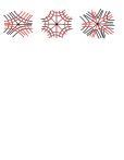
Figure 9. Curvature lines near isolated umbilic points of immersions with constant mean curvature.

3.5. Curvature Lines around Umbilic Curves

In this subsection the results of [34] will be outlined.

The interest on the structure of principal lines in a neighborhood of a continuum of umbilic points, forming a curve, in an analytic surface goes back to the lecture of Carathéodory [5].

Let $c:[0,l]\to\mathbb{R}^{3}$ be a regular curve parametrized by arc length $u$ contained in a regular smooth surface $\mathbb{M}$, which is oriented by the once for all given positive unit normal vector field $N$.

Let $T\circ c=c^{\prime}$. According to Spivak [77], the Darboux frame $\{T,N\wedge T,N\}$ along $c$ satisfies the following system of differential equations:

$$T^{\prime} =k_{g}N\wedge T+k_{n}N$$ (4)

$$(N\wedge T)^{\prime} =-k_{g}T+\tau_{g}N$$

$$N^{\prime} =-k_{n}T-\tau_{g}(N\wedge T)$$

where $k_{n}$ is the normal curvature, $k_{g}$ is the geodesic curvature and $\tau_{g}$ is the geodesic torsion of the curve $c$.

Proposition 1.

Let $c:[0,l]\rightarrow\mathbb{M}$ be a regular arc length parametrization of a curve of umbilic points, such that $\{T,N\wedge T,N\}$ is a positive frame of ${\mathbb{R}}^{3}$. Then the expression

$$\alpha(u,v)=c(u)+v(N\wedge T)(u)+[\frac{1}{2}k(u)v^{2}+\frac{1}{6}a(u)v^{3}+\frac{1}{24}b(u)v^{4}+h.o.t]N(u),$$ (5)

where $k(u)=k_{n}(c(u),T)=k_{n}(c(u),N\wedge T)$ is the normal curvature of $\mathbb{M}$ in the directions $T$ and $N\wedge T$, defines a local $C^{\infty}$ chart in a small tubular neighborhood of $c$. Moreover $\tau_{g}(u)=0$.

The differential equation of curvature lines in the chart $\alpha$ is given by

$$(F g-Gf)dv^{2}+(Eg-Ge)dudv+(Ef-Fe)du^{2}=$$ (6)

$$= Ldv^{2}+Mdvdu+Ndu^{2}=0;$$

$$L= -[k^{\prime}v+\frac{1}{2}(k_{g}k^{\prime}+a^{\prime})v^{2}+\frac{1}{6}(k_{g}a^{\prime}+3k^{\prime}k_{g}^{2}+b^{\prime}+3k^{2}k^{\prime})v^{3}+O(v^{4})]$$

$$M= \;\;a(u)v+\frac{1}{2}[b(u)-3k^{3}-k^{\prime\prime}-3k_{g}a(u)]v^{2}$$

$$+ \frac{1}{6}[15k^{3}k_{g}-3k_{g}^{\prime}k^{\prime}+(3k_{g}^{2}-16k^{2})a(u)-a^{\prime\prime}-5k_{g}b(u)]v^{3}+O(v^{4})$$

$$N= \;k^{\prime}v+\frac{1}{2}(a^{\prime}-3k_{g}k^{\prime})v^{2}+\frac{1}{6}(3k^{\prime}k_{g}^{2}-9k^{2}k^{\prime}-5k_{g}a^{\prime}+b^{\prime})v^{3}+O(v^{4})$$

Proposition 2.

Suppose that $\nabla{\mathcal{H}}(u,0)=(k^{\prime},a(u)/2)$ is not zero at a point $u_{0}$. Then the principal foliations near the point $c(u_{0})$ are as follows.

• If $k^{\prime}(u_{0})\neq 0$ then both principal foliations are transversal to the curve of umbilic points. See Fig. 10, left.

• If $k^{\prime}(u_{0})=0$, $k^{\prime\prime}(u_{0})\neq 0$ and $a(u_{0})\neq 0$, then one principal foliation is transversal to $c$ and the other foliation has quadratic contact with the curve $c$ at the point $c(u_{0})$. See Fig. 10, center and right.

Figure 10. Principal curvature lines near an umbilic curve: transversal case, left, and tangential case, center and right.

Proposition 3.

Suppose that $k^{\prime}(0)=a(0)=0$, $a^{\prime}(0)k^{\prime\prime}(0)\neq 0$, at the point $c(0)$ of a regular curve $c$ of umbilic points. Let $A:=-2k^{\prime\prime}(0)/a^{\prime}(0)\neq 0$ and $B:=[b(0)-3k(0)^{3}-k^{\prime\prime}(0)]/a^{\prime}(0)$. Let $\Delta$ and $\delta$ be defined by

$$\Delta=-4A^{4}+12BA^{3}-(36+12B^{2})A^{2}+(4B^{3}+72B)A-9B^{2}-108;\;\;\delta=2-AB.$$

Then the principal foliations at this point are as follows.

• If $\delta<0$ and $\Delta<0$ then $0$ is topologically equivalent to a Darbouxian umbilic of type D₁, through which the umbilic curve is adjoined transversally to the separatrices. See Fig. 11 left.

• If $\delta<0$ and $\Delta>0$ then $0$ is topologically equivalent to a Darbouxian umbilic of type D₂, through which the umbilic curve is adjoined, on the interior of the parabolic sectors, transversally to the separatrices and to the nodal central line. See Fig. 11 center.

• If $\delta>0$ then $0$ is topologically a Darbouxian umbilic of type D₃, through which the umbilic curve is adjoined transversally to the separatrices. See Fig. 11 right.

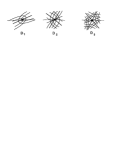
Figure 11. Principal curvature lines near a Darbouxian-like point on an umbilic curve, dotted.

In the previous propositions have been studied a sample of the most generic situations, under the restriction on the surface of having an umbilic curve. Below will be considered the case where $k$ is a constant which implies the additional constrain that the umbilic curve be spherical or planar, a case also partially considered in Carathéodory [5]. Under this double imposition the simplest patterns of principal curvature lines are analyzed in what follows.

Proposition 4.

Let $c$ be a regular closed spherical or planar curve. Suppose that $c$ is a regular curve of umbilic points on a smooth surface. Then the principal foliations near the curve are as follows.

• If ${\mathcal{H}}_{v}(u,0)=a(u)/2\neq 0$ and $a(u)>0$ for definiteness, then one principal foliation is transversal to the curve $c$ of umbilic points.

  The other foliation defines a first return map (holonomy) $\pi$ along the oriented umbilic curve $c$, with first derivative $\pi^{\prime}=1$ and second derivative given by a positive multiple of

  $$\int_{0}^{l}[k_{g}(u){a^{\prime}(u)}/{a(u)^{\frac{3}{2}}}]du.$$

  When the above integral is non zero the principal lines spiral towards or away from $c$, depending on their side relative to $c$.

• If $a(u)$ has only transversal zeros, near them the principal foliations have the topological behavior of a Darbouxian umbilic point D₃ at which a separatrix has been replaced with the umbilic curve. See Fig. 12.

Figure 12. Curvature lines near a spherical umbilic curve.

4. Curvature Lines in the Neighborhood of Critical Points

In this section, following [19], [25] and [47], will be described the local behavior of principal curvature lines near critical points of the surface such as Whitney umbrella critical points, conic critical points and elementary ends of immersions with constant mean curvature.

4.1. Curvature Lines around Whitney Umbrella Critical Points

In this subsection it will be described the behavior of principal lines near critical points of Whitney type of smooth immersions $\alpha:\mathbb{M}\to\mathbb{R}^{3}$.

The mapping $\alpha$ is said to have a Whitney umbrella at $0$ provided it has rank 1 and its first jet extension $j^{1}\alpha$ is transversal to the codimension 2 submanifold $S^{1}(2,3)$ of 1-jets of rank 1 in the space $J^{1}(2,3)$ of 1-jets of smooth mappings of $(\mathbb{R}^{2},0)$ to $(\mathbb{R}^{3},0)$. In coordinates this means that there exist a local chart $(u,v)$ such that $\alpha_{u}(0)\neq 0,\;\;\alpha_{v}(0)=0$ and $[\alpha_{u},\alpha_{uv},\alpha_{vv}]\neq 0$. Here $[.,.,.]$ means the determinant of three vectors.

The structure of a smooth map near such point is illustrated in Fig. 13. It follows from the work of Whitney [81] that these points are isolated and in fact have the following normal form under diffeomorphic changes of coordinates in the source and target ($\mathcal{A}$-equivalence):

$$x=u,\quad y=uv,\quad z=v^{2}.$$

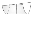
Figure 13. Whitney umbrella critical point.

For the study of principal lines the following proposition is useful.

Proposition 5.

Let $\alpha:(\mathbb{R}^{2},0)\to(\mathbb{R}^{3},0)$ be a $C^{r},\;r\geq 4,$ map with a Whitney umbrella at $0$. Then by the action of the group ${\mathcal{G}}^{k}$ and that of rotations and homoteties of $\mathbb{R}^{3}$, the map $\alpha$ can be written in the following form:

$$\alpha(u,v)=(u,y(u,v),z(u,v))$$

where,

$$y(u,v) =uv+\frac{a}{6}v^{3}+O(4)$$

$$z(u,v) =\frac{b}{2}u^{2}+cuv+v^{2}+\frac{A}{6}u^{3}+\frac{B}{2}u^{2}v+\frac{C}{2}uv^{2}+\frac{D}{6}v^{3}+O(4)$$

and $O(4)$ means terms of order greater than or equal to four.

The differential equation of the lines of curvature of the map $\alpha$ around a Whitney umbrella point $(0,0)$, as in Proposition 5, is given by:

$$[8v^{3}+u\;O(\sqrt{u^{2}+v^{2}})+O(u^{2}+v^{2})]dv^{2}$$

$$+[2u+Cu^{2}+(D-ac)uv-av^{2}+O((u^{2}+v^{2})^{3/2})]dudv$$

$$+[-2v+\frac{B}{2}u^{2}+\frac{1}{2}(ac-D)v^{2}-b^{2}cu^{3}+$$

$$\qquad\qquad\qquad v\;O(\sqrt{u^{2}+v^{2}})+O(u^{2}+v^{2})]du^{2}=0.$$

Theorem 6.

[19] Let $p$ be a Whitney umbrella of a map $\alpha:\mathbb{M}^{2}\to\mathbb{R}^{3}$ of class $C^{k},\;\;k\geq 4$. Then the principal configuration near $p$ has the following structure: Each principal foliation ${\mathcal{F}}_{i}(\alpha)$ of $\alpha$ has exactly two sectors at $p;$ one parabolic and the other hyperbolic. Also, the separatrices of these sectors are tangent to the kernel of $D\alpha_{p}$.

Fig. 14 illustrates the behavior of principal curvature lines near a Whitney umbrella.

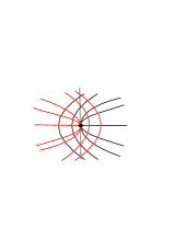
Figure 14. Curvature lines near a Whitney umbrella.

Remark 1.

Global aspects of principal configurations of maps with Whitney umbrellas was carried out in [19].

4.2. Curvature Lines near Conic Critical Points

A surface in Euclidean $\mathbb{R}^{3}$-space is defined implicitly as the variety ${\mathcal{V}}(f)$ of zeroes of a real valued function $f$, assumed of class $C^{k}$.

The points $p\in{\mathcal{V}}(f)$ at which the first derivative $df_{p}$ does not vanish (resp. vanishes) are called regular (resp. critical); they determine the set denoted ${\mathcal{R}}(f)$ (resp. ${\mathcal{C}}(f)$), called the regular or smooth (resp. critical) part of the surface.

The orientation on ${\mathcal{V}}(f)$, or rather ${\mathcal{R}}(f)$, is defined by taking the gradient $\nabla f$ to be the positive normal. In canonical coordinates $(x,y,z)$ it follows that $\nabla f=(f_{x},f_{y},f_{z})$.

The Gaussian normal map $N_{f}$, of ${\mathcal{R}}(f)$ into $\mathbb{S}^{2}$ is defined by $N_{f}=\nabla f/|\nabla f|$.

The eigenvalues $-k^{1}_{f}(p)$ and $-k^{2}_{f}(p)$ of $DN_{f}(p)$, restricted to $T_{p}{\mathcal{R}}(f)$, the tangent space to the surface at $p$, define the principal curvatures, $k^{1}_{f}(p)$ and $k^{2}_{f}(p)$ of the surface at the point $p$. It will be assumed that $k^{1}_{f}(p)\leq k^{2}_{f}(p)$.

The points on ${\mathcal{R}}(f)$ where the two principal curvatures coincide, define the set ${\mathcal{U}}(f)$ of umbilic points of ${\mathcal{V}}(f)$.

On ${\mathcal{R}}(f)\setminus{\mathcal{U}}(f)$, the eigenspaces of $DN_{f}$ associated to $-k^{1}_{f}(p)$ and $-k^{2}_{f}(p)$ define $C^{k-2}$ line fields ${\mathcal{L}}_{1}(f)$ and ${\mathcal{L}}_{2}(f)$, mutually orthogonal, called respectively minimal and maximal principal lines fields of the surface ${\mathcal{V}}(f)$. Their integral curves are called respectively the lines of minimal and maximal principal curvature or, simply the principal lines of ${\mathcal{V}}(f)$.

The integral foliations ${\mathcal{F}}_{1}(f)$ and ${\mathcal{F}}_{2}(f)$ of the lines fields ${\mathcal{L}}_{1}(f)$ and ${\mathcal{L}}_{2}(f)$ are called, respectively, the minimal and maximal foliations of ${\mathcal{V}}(f)$.

The net ${\mathcal{P}}(f)=({\mathcal{F}}_{1}(f),{\mathcal{F}}_{2}(f))$ of orthogonal curves on ${\mathcal{R}}(f)\setminus{\mathcal{U}}(f)$ is called principal net.

A surface ${\mathcal{V}}(f)$ of class $C^{k},\;k\geq 3$, is said to have a non degenerate critical point at $p$ provided that function $f$ vanishes together with its first partial derivatives at $p$ and that the determinant of the Hessian matrix

$$H(f,p)=\left(\begin{matrix}f_{xx}&f_{xy}&f_{xz}\\ f_{xy}&f_{yy}&f_{yz}\\ f_{xz}&f_{yz}&f_{zz}\end{matrix}\right)$$

does not vanish.

The local differentiable structure of ${\mathcal{V}}(f)$, is determined, modulo diffeomorphism, by the number $\nu=\nu(f,p)$ of negative eigenvalues of $H(f,p)$; $\nu$ is called the index of the critical point.

It will be assumed that $\nu=1$ and that in the orthonormal coordinates $(x,y,z)$ the critical point is $0$ such that the diagonal quadratic part of $f$ is given by: $f_{2}(x,y,z)=x^{2}/a^{2}+y^{2}/b^{2}-z^{2}$.

So, $f=f_{2}+f_{3}$ with

$$f_{3}(x,y,z)=\sum_{i+j+k=3}a_{ijk}(x,y,z)x^{i}y^{j}z^{k},$$

where $a_{ijk}$ are functions of class $C^{k-3}$.

Theorem 7.

[25] Let $f_{2}(x,y,z)=x^{2}/a^{2}+y^{2}/b^{2}-z^{2}$ and

$$f_{111}(x,y,z)=f_{2}(x,y,z)+cxyz=0,\quad\sigma=(a-b)c\neq 0.$$

Then ${\mathcal{F}}_{1}(f_{111})$ spirals locally around the critical conic point. See Fig. 15.

The other principal foliation ${\mathcal{F}}_{2}(f_{111})$ preserves locally the radial behavior of ${\mathcal{F}}_{1}(f_{2})$. More precisely, there is a local orientation preserving homeomorphism mapping $\{{\mathcal{V}}(f_{111}),0\}$ to $\{{\mathcal{V}}(f_{2}),0\}$, sending the principal net ${\mathcal{P}}(f_{111})$ on the net ${\mathbb{F}}=({\mathbb{F}_{1}},{\mathbb{F}_{2}})$ on ${\mathcal{V}}(f_{2})$, defined by the integral foliations ${\mathbb{F}_{1}}$ and ${\mathbb{F}_{2}}$ of the vector fields

$$X_{1}=X_{2}-a^{2}y\partial/{\partial x}+b^{2}x\partial/{\partial y},X_{2}=\sigma z(x\partial/{\partial x}+y\partial/{\partial y}+z\partial/{\partial z}).$$

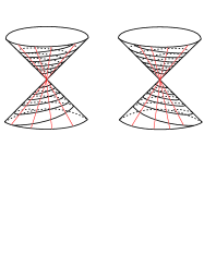
Figure 15. Curvature lines near a critical point of conical type.

Theorem 8.

[25] Let $f$ be of class $C^{k}$, $k\geq 7$, with a non degenerate critical point of index $\nu=1$ at $0$, written as $f=f_{2}+f_{3}$. For $\sigma=(a-b)a_{111}(0)\neq 0$, there is a local orientation preserving homeomorphism mapping $\{{\mathcal{V}}(f),0\}$ to $\{{\mathcal{V}}(f_{111}),0\}$, sending the principal net ${\mathcal{P}}(f)$ on that of ${\mathcal{P}}(f_{111}).$ Here $f_{111}(x,y,z)=f_{2}(x,y,z)+a_{111}(0)xyz$.

Remark 2.

Local and global stability of principal nets ${\mathcal{P}}(f)$ on surfaces defined implicitly were also studied in [25].

4.3. Ends of Surfaces Immersed with Constant Mean Curvature

Let $(u,v):\mathbb{M}\to\mathbb{R}^{2}\setminus\{0\}$ be isothermic coordinates for an immersion $\alpha:\mathbb{M}\to\mathbb{R}^{3}$ with constant mean curvature. If the associated complex function $\phi(w),\;w=u+iv,$ has in zero a pole of order $n\neq 2$, then there exists a small neighborhood $V$ of $0$ in $\mathbb{R}^{2}$ such that the principal lines of $\alpha$, restricted to $(u,v)^{-1}(V\setminus\{0\})$, distribute themselves (modulo topological equivalence) as if the associated complex function were $w^{-n}$.

An end of the immersion $\alpha$ defined by the system of open sets $U_{j}=\{(u,v):u^{2}+v^{2}<1/j,\;j\in\mathbb{N}\}$ where $(u,v)$ are isothermic coordinates for $\alpha$, on which the associated complex function $\phi$ has a pole of order $n$ in $(u,v)=(0,0)$, is called an elementary end of order $n$ of $\alpha$. The index of such an elementary end is $n/2.$

The lines of curvature of an immersion $\alpha$ with constant mean curvature near an elementary end $E$ of order $n$ are described as follows. See more details in [47] and Fig. 16.

• For $n=1$, there is exactly one line $S$ (resp. $s$) of ${\mathcal{F}}_{1}(\alpha)$ (resp. ${\mathcal{F}}_{2}(\alpha)$) which tends to $E$, all the other lines fill a hyperbolic sector bounded by $E$ and $S$ (resp. $s$).

• For $n=2,$ suppose that $\phi(z)$ is the associated complex and $a=\lim_{z\to 0}z^{2}\phi(z).$ There are two cases:

• $a\notin\mathbb{R}\cup(i\mathbb{R})$. Then the lines of ${\mathcal{F}}_{1}(\alpha)$ and ${\mathcal{F}}_{2}(\alpha)$, tend to E.

• $a\in\mathbb{R}\cup(i\mathbb{R})$. Then the lines of ${\mathcal{F}}_{1}(\alpha)$ (resp. ${\mathcal{F}}_{2}(\alpha)$) are circles or rays tending to $E$ and those of ${\mathcal{F}}_{2}(\alpha)$, (resp. ${\mathcal{F}}_{1}(\alpha)$) are rays or circles.

• For $n\geq 3$, every line of ${\mathcal{F}}_{1}(\alpha)$ and ${\mathcal{F}}_{2}(\alpha)$, tends to $E.$ The principal lines distribute themselves into $n-2$ elliptic sectors, two consecutive of which are separated by a parabolic sector.

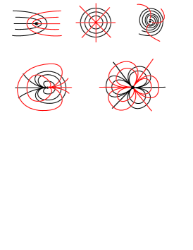
Figure 16. Curvature lines near elementary end points.

5. Curvature Lines near Principal Cycles

A compact leaf $\gamma$ of ${\mathcal{F}}_{1}(\alpha)$ (resp. ${\mathcal{F}}_{2}(\alpha)$) is called a minimal (resp. maximal) principal cycle.

A useful local parametrization near a principal cycle is given by the following proposition and was introduced by Gutierrez and Sotomayor in [43].

Proposition 6.

Let $\gamma:[0,L]\rightarrow{\mathbb{R}}^{3}$ be a principal cycle of an immersed surface $\mathbb{M}$ such that $\{T,N\wedge T,N\}$ is a positive frame of ${\mathbb{R}}^{3}$. Then the expression

$$\alpha(s,v)= \gamma(s)+v(N\wedge T)(s)$$ (7)

$$+ [\frac{1}{2}k_{2}(s)v^{2}+\frac{1}{6}b(s)v^{3}+o(v^{3})]N(s),\;\;-\delta<v<\delta$$

where $k_{2}$ is the principal curvature in the direction of $N\wedge T$, defines a local $C^{\infty}$ chart on the surface ${\mathbb{M}}$   defined in a small tubular neighborhood of $\gamma$.

Remark 3.

Calculation shows that the following relations hold

$$k_{g}(s)=-\frac{(k_{1})_{v}}{k_{2}-k_{1}},\;\;k_{g}^{\perp}(s)=-\frac{(k_{2})^{\prime}}{k_{2}-k_{1}},\;\;\;\;\;b(s)=(k_{2})_{v}=\frac{\partial k_{2}}{\partial v}$$ (8)

Here $k_{g}^{\perp}(s)$ is the geodesic curvature of the maximal principal curvature line which pass through $\gamma(s)$.

Proposition 7 (Gutierrez-Sotomayor).

[43] Let $\gamma$ be a minimal principal cycle of an immersion $\alpha:\mathbb{M}\to\mathbb{R}^{3}$ of length $L$. Denote by $\pi_{\alpha}$ the first return map associated to $\gamma$. Then

$$\pi^{\prime}_{\alpha}(0)= exp[\int_{\gamma}\frac{-dk_{2}}{k_{2}-k_{1}}]=exp[\int_{\gamma}k_{g}^{\perp}(s)ds]$$ (9)

$$= exp[\int_{\gamma}\frac{-dk_{1}}{k_{1}-k_{2}}]=exp[\frac{1}{2}\int_{\gamma}\frac{d{\mathcal{H}}}{\sqrt{{\mathcal{H}}^{2}-{\mathcal{K}}}}].$$

The following result established in [46] is improved in the next proposition.

Proposition 8.

Let $\gamma$ be a minimal principal cycle of length $L$ of a surface $\mathbb{M}\subset\mathbb{R}^{3}$. Consider a chart $(s,v)$ in a neighborhood of $\gamma$ given by equation (7). Denote by $k_{1}$ and $k_{2}$ the principal curvatures of $\mathbb{M}$. Let $Jac(k_{1},k_{2})=\frac{\partial(k_{1},k_{2})}{\partial(s,v)}=(k_{1})_{s}(k_{2})_{v}-(k_{1})_{v}(k_{2})_{s}$ and suppose that $\gamma$ is not hyperbolic, i.e. the first derivative of the first return map $\pi$ associated to $\gamma$ is one. Then the second derivative of $\pi$ is given by:

$$\pi^{\prime\prime}(0)=\int_{0}^{L}e^{-\int_{0}^{s}\frac{k_{2}^{\prime}}{k_{2}-k_{1}}du}\frac{Jac(k_{1},k_{2})}{(k_{2}-k_{1})^{2}}ds.$$

Theorem 9.

[24, 26] For a principal cycle $\gamma$ of multiplicity $n$, $1\leq n<\infty$, there is a chart $(u,v)$ with $c=\{v=0\}$, such that the principal lines are given by

$$du= 0,\;\;dv-a_{1}vdu,\;a_{1}\in\mathbb{R},\;\text{for}\;n=1.$$

$$du= 0,\;\;dv-v^{n}(a_{n}-{a}_{2n-1}v^{n-1})du=0;\;\;a_{n},a_{2n-1}\in\mathbb{R},\;\text{and }\;n\geq 2.$$

Here, the numbers $a_{1}$, $a_{n}$ and ${a}_{2n-1}$ are uniquely determined by the jet of order $2n+1$ of immersion $\alpha$ along $\gamma$ and can be expressed in terms of integrals involving the principal curvatures $k_{1}(u,v)$ and $k_{2}(u,v)$ and its derivatives.

The next result establishes how a principal cycle of multiplicity $n$, $2\leq n<\infty,$ of an immersion $\alpha$ splits under deformations $\alpha_{\epsilon}$.

Recall from [37] that a family of functions $\;U(.,\epsilon),\;$ $\epsilon\in\mathbb{R}^{n},$ is an universal unfolding of $U(.,0)$ if for any deformation $H(.,\theta),$ $\theta\in\mathbb{R}^{l}$ of $U(.,0),$ the following equation $\;H(v,\theta)=S(v,\theta)U(\beta(v,\theta),\lambda(\theta))\;$ holds.

Here $\;S,\;$ $\beta\;$ and $\,\lambda\,$ are $C^{\infty}$ functions with $\,S(v,\theta)>0,\,$ $\beta(v,0)=v$, $\;\lambda(0)=0$. Furthermore it is required that $n$ is the minimal number with this property.

For a minimal principal cycle $\gamma$ of $\alpha$ on which $k_{1}$ is not constant consider the following deformation:

$${\alpha}_{\epsilon}=\alpha+k_{1}^{\prime}(u)\delta(v)\big{(}\sum_{i=1}^{n-1}{\epsilon}_{i}\frac{v^{i}}{i!}\big{)}N_{\alpha}(u).$$

Here $v$ is a $C^{\infty}$ function on M such that $v{|}_{c}=0$, ${\nabla}_{\alpha}v$ is a unit vector on the induced metric ${<,>}_{a}$; ${\nabla}_{\alpha}$ denotes the gradient relative to this metric and $\delta$ is a non negative function, identically $1$ on a neighborhood of $\gamma,$ whose support is contained on the domain of $v$.

Theorem 10.

[26] For a minimal principal cycle $\gamma$ of multiplicity n, $2\leq n<\infty,$ of $\alpha$, on which the principal curvature $k_{1}$ is not a constant, the following holds.

The function $U(x,\epsilon)={\pi}_{{\alpha}_{\epsilon}}(x)-x$ provides a universal unfolding for $U(.,0)={\pi}_{\alpha}-id$. Here ${\pi}_{{\alpha}_{\epsilon}}$ denotes the return map of the deformation ${\alpha}_{\epsilon}$.

Remark 4.

• Principal cycles on immersed surfaces with constant mean curvature was studied in [47]. There is proved that the Poincaré transition map preserves a transversal measure and the principal cycles appears in open sets, i.e. they fill an open region.

• Principal cycles on immersed Weingarten surfaces have been studied in [73]. They also appear in open sets.

• In [24] was established an integral expression for $\pi^{\prime}$ in terms of the principal curvatures and the Riemann Curvature Tensor of the manifold in which the surface is immersed. It seems challenging to discover the general pattern for the higher derivatives of the return map in this case.

6. Curvature Lines on Canal Surfaces

In this section it will determined the principal curvatures and principal curvature lines on canal surfaces which are the envelopes of families of spheres with variable radius and centers moving along a closed regular curve in $\mathbb{R}^{3}$, see [80]. This study were carried out in [21].

Consider the space $\mathbb{R}^{3}$ endowed with the Euclidean inner product $<\,,\,>$ and norm $|\,\,\,|=<\,,\,>^{1/2}$ as well as with a canonical orientation.

Let ${\mathbf{c}}$ be a smooth regular closed curve immersed in $\mathbb{R}^{3}$, parametrized by arc length $s\in[0,L]$. This means that

$${\mathbf{c}}^{\prime}(s)={\mathbf{t}}(s),\;|{\mathbf{t}}(s)|=1,\;{\mathbf{c}}(L)={\mathbf{c}}(0)\;.$$ (10)

Assume also that the curve is bi-regular. That is:

$$\kappa(s)=|{\mathbf{t}}^{\prime}(s)|>0.$$ (11)

Along ${\mathbf{c}}$ is defined its moving Frenet frame $\{{\mathbf{t}},{\mathbf{n}},{\mathbf{b}}\}$. Following Spivak [77] and Struik [78], this frame is positive, orthonormal and verifies Frenet equations:

$${\mathbf{t}}^{\prime}(s)=\kappa(s){\mathbf{n}}(s),\;{\mathbf{n}}^{\prime}(s)=-\kappa(s){\mathbf{t}}(s)+\tau(s){\mathbf{b}}(s),\;{\mathbf{b}}^{\prime}(s)=-\tau(s){\mathbf{n}}(s).$$ (12)

Equations (10) to (12) define the unit tangent, ${\mathbf{t}}$, principal normal, ${\mathbf{n}}$, curvature, $\kappa$, binormal, ${\mathbf{b}}={\mathbf{t}}\wedge{\mathbf{n}}$, and torsion, $\tau$, of the immersed curve ${\mathbf{c}}$.

Proposition 9.

Let $r(s)>0$ and $\theta(s)\in\;]0,\pi[$ be smooth functions of period $L$. The mapping $\alpha:\mathbb{T}^{2}=\mathbb{S}^{1}\times\mathbb{S}^{1}\to\mathbb{R}^{3},$ defined on $\mathbb{R}^{2}$ modulo $L\times 2\pi$ by

$$\alpha(s,\varphi)={\mathbf{c}}(s)+r(s)\cos\theta(s){\mathbf{t}}(s)+r(s)\sin\theta(s)[\cos\varphi\,{\mathbf{n}}(s)+\sin\varphi\,{\mathbf{b}}(s)],$$ (13)

is tangent to the sphere of center ${\mathbf{c}}(s)$ and radius $r(s)$ if and only if

$$\cos\theta(s)=-r^{\prime}(s).$$ (14)

Assuming (14), with $r^{\prime}(s)<1$, $\alpha$ is an immersion provided

$$\kappa(s)<\frac{1-r^{\prime}(s)^{2}-r(s)r^{\prime\prime}(s)}{r(s)\sqrt{1-r^{\prime}(s)^{2}}}.$$ (15)

Definition 1.

A mapping such as $\alpha$, of $\,\,{\mathbb{T}}^{2}$ into $\mathbb{R}^{3}$, satisfying conditions (14) and (15) will be called an immersed canal surface with center along ${\mathbf{c}}(s)$ and radial function $r(s)$. When $r$ is constant, it is called an immersed tube. Due to the tangency condition (14), the immersed canal surface $\alpha$ is the envelope of the family of spheres of radius $r(s)$ whose centers range along the curve ${\mathbf{c}}(s)$.

Theorem 11.

Let $\alpha:{\mathbb{S}}^{1}\times{\mathbb{S}}^{1}\to{\mathbb{R}}^{3}$ be a smooth immersion expressed by (13). Assume the regularity conditions (14) and (15) as in Proposition 9 and also that

$$k(s)<\Big{|}\frac{1-r^{\prime}(s)^{2}-2r(s)r^{\prime\prime}(s)}{2r(s)\sqrt{1-r^{\prime}(s)^{2}}}\Big{|}.$$ (16)

The maximal principal curvature lines are the circles tangent to $\partial/\partial\varphi$. The maximal principal curvature is

$$k_{2}(s)=1/r(s).$$

The minimal principal curvature lines are the curves tangent to

$$V(s,\varphi)=\frac{\partial}{\partial s}-\left(\tau(s)+\frac{r^{\prime}(s)}{(1-r^{\prime}(s)^{2})^{1/2}}\kappa(s)\sin\varphi\right)\frac{\partial}{\partial\varphi}.$$ (17)

The expression

$$r(s)(1-r^{\prime}(s)^{2})^{1/2}\kappa(s)\cos\varphi+r(s)r^{\prime\prime}(s)-(1-r^{\prime}(s)^{2})$$ (18)

is negative, and the minimal principal curvature is given by

$$k_{1}(s,\varphi)=\frac{\kappa(s)(1-r^{\prime}(s)^{2})^{1/2}\cos\varphi+r^{\prime\prime}(s)}{r(s)(1-r^{\prime}(s)^{2})^{1/2}\kappa(s)\cos\varphi+r(s)r^{\prime\prime}(s)-(1-r^{\prime}(s)^{2})}.$$ (19)

There are no umbilic points for $\alpha$: $k_{1}(s,\varphi)<k_{2}(s).$

Remark 5.

A consequence of the Riccati structure for principal curvature lines on canal immersed surfaces established in Theorem 11 implies that the maximal number of isolated periodic principal lines is $2$. Examples of canal surfaces with two (simple i.e. hyperbolic) and one (double i.e. semi–stable) principal periodic lines were developed in [21].

7. Curvature Lines near Umbilic Connections and Loops

A principal line $\gamma$ which is an umbilic separatrix of two different umbilic points $p$, $q$ of $\alpha$ or twice a separatrix of the same umbilic point $p$ of $\alpha$ is called an umbilic separatrix connection of $\alpha$; in the second case $\gamma$ is also called an umbilic separatrix loop. The simplest bifurcations of umbilic connections, including umbilic loops, as well as the consequent appearance of principal cycles will be outlined below, following [49] and [20].

There are three types of umbilic connections, illustrated in Fig. 17, from which principal cycles bifurcate. They are defined as follows:

$\bullet$ $C_{11}$-simple connection, which consists in two D₁ umbilics joined by their separatrix, whose return map $T$ has first derivative $T^{\prime}\neq 1$. In [49] this derivative is expressed in terms of the third order jet of the surface at the umbilics.

$\bullet$ $C_{22}$-simple loop, which consists in one D₂ umbilic point self connected by a separatrix, whose return map $T$ verifies $\lim_{x\to 0+}\log(T(x))/\log(x)\neq 1$. In [49] this derivative is expressed in terms of the third order jet of the surface at the umbilic.

$\bullet$ $C_{33}$-simple loop, the same as above exchanging D₂ by D₃ umbilic point.

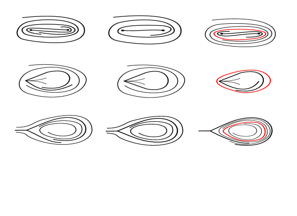
Figure 17. Simple Connection and Loops and their Bifurcations: $C_{11}$, top, $C_{22}$, middle and $C_{33}$, bottom.

Below will be outlined the results obtained in [20].

There are two bifurcation patterns producing principal cycles which are associated with the bifurcations of D${}^{1}_{2}$ and D${}^{1}_{2,3}$ umbilic points, when their separatrices form loops, self connecting these points. They are defined as follows.

$\bullet$ A D${}^{1}_{2}$ - interior loop consists on a point of type D${}^{1}_{2}$ and its isolated separatrix, which is assumed to be contained in the interior of the parabolic sector. See Fig. 18, where such loop together with the bifurcating principal cycle are illustrated. Here, a hyperbolic principal cycle bifurcates from the loop when the D${}^{1}_{2}$ point bifurcates into D₁ .

Figure 18. D${}^{1}_{2}$ - loop bifurcation.

If both principal foliations have D${}^{1}_{2}$ - interior loops (at the same D${}^{1}_{2}$ point), after bifurcation there appear two hyperbolic cycles, one for each foliation. This case will be called double D${}^{1}_{2}$ - interior loop. In Fig. 19, Fig. 18 has been modified and completed accordingly so as to represent both maximal and minimal foliations, each with its respective D${}^{1}_{2}$ -interior loops (left) and bifurcating hyperbolic principal cycles (right).

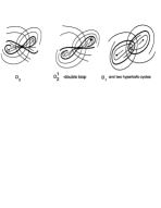
Figure 19. D${}^{1}_{2}$ - double loop bifurcation.

$\bullet$ A D${}^{1}_{2,3}$ - interior loop consists on a point of type D${}^{1}_{2,3}$ and its hyperbolic separatrix, which is assumed to be contained in the interior of the parabolic sector. See Fig. 20, where such loop together with the bifurcating principal cycle are illustrated. Here, a unique hyperbolic principal cycle bifurcates from the loop when the umbilic points are annihilated.

Figure 20. D${}^{1}_{2,3}$ - loop bifurcation.

8. Principal Configurations on Algebraic Surfaces in $\mathbb{R}^{3}$

An algebraic surface of degree $n$ in Euclidean $(x_{1},x_{2},x_{3})$-space $\mathbb{R}^{3}$ is defined by the variety $A(\alpha)$ of real zeros of a polynomial $\alpha$ of the form $\alpha=\sum\alpha_{h},\,h=0,\,1,\,2,...,n$, where $\alpha_{h}$ is a homogeneous polynomial of degree $h$: $\alpha_{h}=\sum a_{ijk}x_{1}^{i}x_{2}^{j}x_{3}^{k},\,i+j+k=h$, with real coefficients.

An end point or point at infinity of $A(\alpha)$ is a point in the unit sphere $\mathbb{S}^{2}$, which is the limit of a sequence of the form $p_{n}/|p_{n}|$, for $p_{n}$ tending to infinity in $A(\alpha).$

The end locus or curve at infinity of $A(\alpha)$ is defined as the collection $E(\alpha_{n})$ of end points of $A(\alpha).$ Clearly, $E(\alpha)$ is contained in the algebraic set $E(\alpha)=\{p\in\mathbb{S}^{2};\alpha(p)=0\},\;$ called the algebraic end locus of $A(\alpha).$

A surface $A(\alpha)$ is said to be regular (or smooth) at infinity if $0$ is a regular value of the restriction of $\alpha_{n}$ to $\mathbb{S}^{2}.$ This is equivalent to require that $\nabla\alpha_{n}(p)\wedge p$ does not vanish whenever $\alpha_{n}(p)=0,$ $p\neq 0$. In this case, clearly $E(\alpha)=E_{n}(\alpha)$ and, when non empty, it consists of a finite collection $\{\gamma_{i};\,\,i=1,\ldots,k(\alpha_{n})\}$ of smooth closed curves, called the (regular) curves at infinity of $A(\alpha)$; this collection of curves is invariant under the antipodal map, $a:p\to-p,$ of the sphere.

There are two types of curves at infinity: odd curves if $a(\gamma_{i})=\gamma_{i}$, and even curves if $\gamma_{j}=a(\gamma_{i})$ is disjoint from $\gamma_{i}$ .

A regular end point $p$ of $A(\alpha)$ in $\mathbb{S}^{2}$ will be called an ordinary or biregular end point of $A(\alpha)$ if the geodesic curvature, $k_{g}$, of the curve $E(\alpha)$ at $p$, considered as a spherical curve, is different from zero; it is called singular or inflexion end point if $k_{g}$ is equal to zero.

An inflexion end point $p$ of a surface $A(\alpha)$ is called bitransversal, provided the following two transversality conditions hold:

$$(T_{1})\;\;\;\;\;\;\;\;\;\;\;\;\;\;\;\;k_{g}^{\prime}(p)=dk_{g}(p;\tau)\neq 0$$

and

$$(T_{2})\;\;\;\;\;\;\;\;\;\nu(p)=d[\alpha_{n-1}/|\nabla\alpha_{n}|](p;\tau)\neq 0.$$

There are two different types of bitransversal inflexion end points, illustrated in Fig. 2: hyperbolic if $k_{g}^{\prime}.\nu<0$ and elliptic if $k_{g}^{\prime}.\nu>0.$

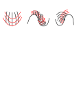
Figure 21. Principal nets near biregular (left) and bitransversal end points (hyperbolic, center, and elliptic, right).

A regular end curve $\gamma$ all whose points are biregular, i.e. $\gamma$ is free from inflexion points, will be called a principal cycle at infinity; it will be called semi-hyperbolic if

$$\eta=\int_{\gamma}\alpha_{n-1}|\nabla\alpha_{n}|^{-1}d(k_{g}^{-1})\neq 0.$$

Little is know about the structure of principal nets on algebraic surfaces of degree $n$. The case of quadrics $(n=2),$ where the principal nets are fully known, is a remarkable exception, whose study goes back to the classical works of Monge [60], Dupin [7], and Darboux [6], among others. See the discussion in section 2 and also [77], [78].

The description of their principal nets in terms of intersections of the surface with other families of quadrics in triply orthogonal ellipsoidal coordinate systems, appear in most differential geometric presentations of surface theory, notably Struik’s and Spivak’s [78], [77]. Also, Geometry books of general expository character, such as Fischer [10] and Hilbert-Cohn Vossen [54], also explain these properties of quadrics and include pictorial illustrations of their principal nets.

For algebraic surfaces of degrees three (cubics), four (quartics) and higher, however, nothing concerning principal nets, specific to their algebraic character, seems to be known.

Consider the vector space ${\mathcal{A}}_{n}$ of all polynomials of degree less than or equal to $n$, endowed with the structure of ${\mathbb{R}}^{N}$ -space defined by the $N=N(n)$ coefficients of the polynomials $\alpha.$ Here $N(n)=(n+1)(n+2)(n+3)/6.$ The distance in the space ${\mathcal{A}}_{n}$ will be denoted $d_{n}(.,.).$

Structural Stability for (the principal net of) an algebraic surface $A(\alpha)$ of degree $n$ means that there is an $\epsilon>0$ such that for any $\beta$ with $d(\alpha,\beta)<\epsilon$ there is a homeomorphism $h$ from $A(\alpha)$ onto $A(\beta)$ mapping $U(\alpha)$ to $U(\beta)$ and also mapping the lines of ${\mathcal{F}}_{1}(\alpha)$ and ${\mathcal{F}}_{2}(\alpha)$ onto those of ${\mathcal{F}}_{1}(\beta)$ and ${\mathcal{F}}_{2}(\beta)$, respectively.

Denote by $\Sigma_{n}$ the class of surfaces $A(\alpha),\;\alpha\in{\mathcal{A}}_{n}$, which are regular and regular at infinity and satisfy simultaneously that:

• All its umbilic points are Darbouxian and all inflexion ends are bitransversal.

• All its principal cycles are hyperbolic and all biregular end curves, i.e. cycles at infinity, are semi-hyperbolic.

• There are no separatrix connections (outside the end locus) of umbilic and inflexion end points.

• The limit set of any principal line is a principal cycle (finite or infinite), an umbilic point or an end point.

These conditions extend to algebraic surfaces of degree $n$, $n\geq 3$, the conditions given by Gutierrez and Sotomayor in [43, 44, 48], which imply principal stability for compact surfaces.

Theorem 12.

[27] Suppose that $n\geq 3$. The set $\Sigma_{n}$ is open in ${\mathcal{A}}_{n}$, and any surface $A(\alpha)$ on it is principally structurally stable.

Remark 6.

• For $n=2$ the stable surfaces are characterized, after Dupin’s Theorem, by the ellipsoids and hyperboloid of two sheets with different axes and by hyperboloid of one sheet (no conditions on the axes). See Theorem 1.

• By approximating, in the $C^{3}$ topology, the compact principal structurally stable surfaces of Gutierrez and Sotomayor [43, 44, 48] by algebraic ones, can be obtained examples of algebraic surfaces (of undefined degree), which are principally structurally stable on a compact connected component.

  In this form all the patterns of stable principal configurations of compact smooth surfaces are realized by algebraic ones, whose degrees, however, are not determined.

To close this section an open problem is proposed.

Problem 3.

Determine the class of principally structurally stable cubic and higher degree surfaces. In other words, prove or disprove the converse of 12.

Prove the density of $\Sigma_{n}$ in ${\mathcal{A}}_{n}$, for $n=3$ and higher.

Theorem 1 in section 2.1 deals with the case of degree 2 —quadric— surfaces.

9. Axial Configurations on Surfaces Immersed in ${\mathbb{R}}^{4}$

Landmarks of the Curvature Theory for surfaces in ${\mathbb{R}}^{4}$ are the works of Wong [82] and Little [57], where a review of properties of the Second Fundamental Form, the Ellipse of Curvature (defined as the image of this form on unit tangent circles) and related geometric and singular theoretic notions are presented. These authors give a list of pertinent references to original sources previous to 1969, to which one must add that of Forsyth [12]. Further geometric properties of surfaces in $\mathbb{R}^{4}$ have been pursued by Asperti [2] and Fomenko [11], among others.

For an immersion $\alpha$ of a surface $\mathbb{M}$ into ${\mathbb{R}}^{4}$, the axiumbilic singularities ${\mathbb{U}}_{\alpha}$, at which the ellipse of curvature degenerates into a circle, and the lines of axial curvature are assembled into two axial configurations: the principal axial configuration: ${\mathbb{P}}_{\alpha}=\{{\mathbb{U}}{{}_{\alpha}},\;{\mathbb{X}}_{\alpha}\}$ and the mean axial configuration: ${\mathbb{Q}}_{\alpha}=\{{\mathbb{U}}{{}_{\alpha}},\;{\mathbb{Y}}_{\alpha}\}.$

Here, $\mathbb{P}_{\alpha}$= $\{\mathbb{U}{{}_{\alpha}},\;\mathbb{X}_{\alpha}\}$ is defined by the axiumbilics $\mathbb{U}_{\alpha}$ and the field of orthogonal tangent lines $\mathbb{X}_{\alpha}$, on $\mathbb{M}\backslash\mathbb{U}_{\alpha}$, on which the immersion is curved along the large axis of the curvature ellipse. The reason for the name given to this object is that for surfaces in $\mathbb{R}^{3}$, $\mathbb{P}_{\alpha}$ reduces to the classical principal configuration defined by the two principal curvature direction fields $\{\mathbb{X}_{\alpha 1},\mathbb{X}_{\alpha 2}\}$, [43, 48]. Also, in ${\mathbb{Q}}_{\alpha}=\{\mathbb{U}{{}_{\alpha}},\;\mathbb{Y}_{\alpha}\}$, $\mathbb{Y}_{\alpha}$ is the field of orthogonal tangent lines $\mathbb{Y}_{\alpha}$ on $\mathbb{M}\backslash\mathbb{U}_{\alpha}$, on which the immersion is curved along the small axis of the curvature ellipse. For surfaces in $\mathbb{R}^{3}$ the curvature ellipse reduces to a segment and the crossing $\mathbb{Y}_{\alpha}$ splits into the two mean curvature line fields $\{\mathbb{Y}_{\alpha 1},\mathbb{Y}_{\alpha 2}\}$. In this case $\mathbb{Q}_{\alpha}$ reduces to the mean configuration defined by umbilic points and line fields along which the normal curvature is equal to the Mean Curvature. That is the arithmetic mean of the principal curvatures.

The global aspects of arithmetic mean configurations of surfaces immersed in $\mathbb{R}^{3}$ have been studied by Garcia and Sotomayor in [30]. Examples of quadratic ellipsoids such that all arithmetic mean curvature lines are dense were given.

Other mean curvature functions have been studied by Garcia and Sotomayor in [31, 32, 33], unifying the arithmetic, geometric and harmonic classical means of the principal curvatures.

The global generic structure of the axial principal and mean curvature lines, along which the second fundamental form points in the direction of the large and the small axes of the Ellipse of Curvature was developed by Garcia and Sotomayor, [29].

A partial local attempt in this direction has been made by Gutierrez et al. in the paper [41], where the structure around the generic axiumbilic points (for which the ellipse is a circle) is established for surfaces smoothly immersed in $\mathbb{R}^{4}$. See Fig. 22 for an illustration of the three generic types: $E_{3},\;E_{4},\;E_{5}$, established in [41] and also in [29].

These points must regarded as the analogous to the Darbouxian umbilics: D₁,  D₂,  D₃, [6] , [43, 48]. In both cases, the subindices refer to the number of separatrices approaching the singularity.

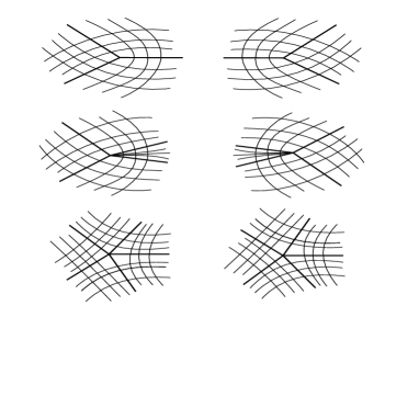
Figure 22. Axial configuration near axiumbilic points.

9.1. Differential equation for lines of axial curvature

Let $\alpha:\mathbb{M}^{2}\to\mathbb{R}^{4}$ be a $C^{r},\;\;r\geq 4,$ immersion of an oriented smooth surface $\mathbb{M}$ into $\mathbb{R}^{4}$. Let $N_{1}$ and $N_{2}$ be a frame of vector fields orthonormal to $\alpha$. Assume that $(u,v)$ is a positive chart and that $\{\alpha_{u},\alpha_{v},N_{1},N_{2}\}$ is a positive frame.

In a chart $(u,v)$, the first fundamental form of $\alpha$ is given by:

$I_{\alpha}=<D\alpha,D\alpha>=Edu^{2}+2Fdudv+Gdv^{2}$, with

$E=<\alpha_{u},\alpha_{u}>$, $F=<\alpha_{u},\alpha_{v}>$, $G=<\alpha_{v},\alpha_{v}>$

The second fundamental form is given by:

$$II_{\alpha}=II_{1,\alpha}N_{1}+II_{2,\alpha}N_{2}$$

where,

$II_{1,\alpha}=<N_{1},D^{2}\alpha>=e_{1}du^{2}+2f_{1}dudv+g_{1}dv^{2}$ and

$II_{2,\alpha}=<N_{2},D^{2}\alpha>=e_{2}du^{2}+2f_{2}dudv+g_{2}dv^{2}$.

The normal curvature vector at a point $p$ in a tangent direction $v$ is given by:

$k_{n}=k_{n}(p,v)=II_{\alpha}(v,v)/I_{\alpha}(v,v).$

Denote by $T\mathbb{M}$ the tangent bundle of $\mathbb{M}$ and by $N\mathbb{M}$ the normal bundle of $\alpha$. The image of the unitary circle of $T_{p}\mathbb{M}$ by $k_{n}(p):T_{p}\mathbb{M}\to N_{p}\mathbb{M}$, being a quadratic, map is either an ellipse, a point or a segment. In any case, to unify the notation, it will be refereed to as the ellipse of curvature of $\alpha$ and denoted by $\mathbb{E}_{\alpha}$.

The mean curvature vector ${\mathcal{H}}$ is defined by:

$${\mathcal{H}}=h_{1}N_{1}+h_{2}N_{2}=\frac{Eg_{1}+e_{1}G-2f_{1}F}{2(EG-F^{2})}N_{1}+\frac{Eg_{2}+e_{2}G-2f_{2}F}{2(EG-F^{2})}N_{2}.$$

Therefore, the ellipse of curvature $\mathbb{E}_{\alpha}$ is given by the image of:

$$k_{n}=(k_{n}-{\mathcal{H}})+{\mathcal{H}}.$$

The tangent directions for which the normal curvature are the axes, or vertices, of the ellipse of curvature $\mathbb{E}_{\alpha}$ are characterized by the following quartic form given by the Jacobian of the pair of forms below, the first being quartic and the second quadratic:

$$Jac(||k_{n}-{\mathcal{H}}||^{2},I_{\alpha})=0.$$

where,

$$||k_{n}-{\mathcal{H}}||^{2} =\big{[}\frac{e_{1}du^{2}+2f_{1}dudv+g_{1}dv^{2}}{Edu^{2}+2Fdudv+Gdv^{2}}-\frac{(Eg_{+}e_{1}G-2f_{1}F)}{2(EG-F^{2})}\big{]}^{2}$$

$$+\big{[}\frac{e_{2}du^{2}+2f_{2}dudv+g_{2}dv^{2}}{Edu^{2}+2Fdudv+Gdv^{2}}-\frac{(Eg_{2}+e_{2}G-2f_{2}F)}{2(EG-F^{2})}\big{]}^{2}.$$

Expanding the equation above, it follows that the differential equation for the corresponding tangent directions, which defines the axial curvature lines, is given by a quartic differential equation:

$$A (u,v,du,dv)=[a_{0}G(EG-4F^{2})+a_{1}F(2F^{2}-EG)]dv^{4}$$ (20)

$$+ [-8a_{0}EFG+a_{1}E(4F^{2}-EG)]dv^{3}du$$

$$+ [-6a_{0}GE^{2}+3a_{1}FE^{2}]dv^{2}du^{2}+a_{1}E^{3}dvdu^{3}+a_{0}E^{3}du^{4}=0$$

where,

$$a_{1}= 4G(EG-4F^{2})(e_{1}^{2}+e_{2}^{2})+32EFG(e_{1}f_{1}+e_{2}f_{2})$$

$$+ 4E^{3}(g_{1}^{2}+g_{2}^{2})-8E^{2}G(e_{1}g_{1}+e_{2}g_{2})-16E^{2}G(f_{1}^{2}+f_{2}^{2})$$

$$a_{0}= 4F(EG-2F^{2})(e_{1}^{2}+e_{2}^{2})-4E(EG-4F^{2})(e_{1}f_{1}+e_{2}f_{2})$$

$$- 8E^{2}F(f_{1}^{2}+f_{2}^{2})-4E^{2}F(e_{1}g_{1}+e_{2}g_{2})+4E^{3}(f_{1}g_{1}+f_{2}g_{2}).$$

Remark 7.

Suppose that the surface $\mathbb{M}$ is contained into $\mathbb{R}^{3}$ with $e_{2}=f_{2}=g_{2}=0$. Then the differential equation (20) is the product of the differential equation of its principal curvature lines and the differential equation of its mean curvature lines, i.e., the quartic differential equation (20) is given by

$$Jac(II_{\alpha},I_{\alpha}).Jac(Jac(II_{\alpha},I_{\alpha}),I_{\alpha})=0.$$

Let $\mathbb{M}^{2}$ be a compact, smooth and oriented surface. Call ${\mathcal{M}}^{k}$ the space of $C^{k}$ immersions of $\mathbb{M}^{2}$ into $\mathbb{R}^{4}$, endowed with the $C^{k}$ topology.

An immersion $\alpha\in{\mathcal{M}}^{k}$ is said to be Principal Axial Stable if it has a $C^{k}$, neighborhood ${\mathcal{V}}(\alpha)$, such that for any $\beta\in\mathcal{V}(\alpha)$ there exist a homeomorphism $h:\mathbb{M}^{2}\to\mathbb{M}^{2}$ mapping $\mathbb{U}_{\alpha}$ onto $\mathbb{U}_{\beta}$ and mapping the integral net of $\mathbb{X}_{\alpha}$ onto that of $\mathbb{X}_{\beta}$. Analogous definition is given for Mean Axial Stability.

Sufficient conditions are provided to extend to the present setting the Theorem on Structural Stability for Principal Configurations due to Gutierrez and Sotomayor [43, 44, 48]. Consider the subsets $\mathcal{P}^{k}$ (resp. $\mathcal{Q}^{k}$) of immersions $\alpha$ defined by the following conditions:

• all axiumbilic points are of types: $E_{3}$, $E_{4}$ or $E_{5}$;

• all principal (resp. mean) axial cycles are hyperbolic;

• the limit set of every axial line of curvature is contained in the set of axiumbilic points and principal (resp. mean) axial cycles of $\alpha$;

• all axiumbilic separatrices are associated to a single axiumbilic point; this means that there are no connections or self connections of axiumbilic separatrices.

Theorem 13.

[29] Let $k\geq 5$. The following holds:

• The subsets ${\mathcal{P}}^{k}$ and ${\mathcal{Q}}^{k}$ are open in ${\mathcal{M}}^{k}$;

• Every $\alpha\in{\mathcal{P}}^{k}$ is Principal Axial Stable;

• Every $\alpha\in{\mathcal{Q}}^{k}$ is Mean Axial Stable.

Remark 8.

Several other extensions of principal lines of surfaces immersed in $\mathbb{R}^{4}$ have been considered. To have an idea of these developments the reader is addressed to [22], [23], [40], [58], [67].

10. Principal Configurations on Immersed Hypersurfaces in $\mathbb{R}^{4}$

Let $\mathbb{M}^{m}$ be a $C^{k},k\geq 4$, compact and oriented, $m-$ dimensional manifold. An immersion $\alpha$ of $\mathbb{M}^{m}$ into $\mathbb{R}^{m+1}$ is a map such that $D{\alpha}_{p}:T\mathbb{M}^{m}_{p}\to\mathbb{R}^{m+1}$ is one to one, for every $p\in\mathbb{M}^{m}$. Denote by ${\mathcal{J}}^{k}={\mathcal{J}}^{k}(\mathbb{M}^{m},\mathbb{R}^{m+1})$ the set of $C^{k}$ - immersions of $\mathbb{M}^{m}$ into $\mathbb{R}^{m+1}$. When endowed with the $C^{s}-$ topology of Whitney, $s\leq k,$ this set is denoted by ${\mathcal{J}}^{k,s}$. Associated to every $\alpha\in{\mathcal{J}}^{k}$ is defined the normal map $N_{\alpha}:\mathbb{M}^{m}\to S^{m}$ :

$$N_{\alpha}=({{\alpha}_{1}\wedge\ldots\wedge{\alpha}_{m}})/{\mid{\alpha}_{1}\wedge\ldots\wedge{\alpha}_{m}\mid},$$

where $({u_{1}},\ldots,{u_{m}}):(M,p)\to(\mathbb{R}^{m},0)$ is a positive chart of $\mathbb{M}^{m}$ around p, $\wedge$ denotes the exterior product of vectors in $\mathbb{R}^{m+1}$ determined by a once for all fixed orientation of $\mathbb{R}^{m+1}$, ${\alpha}_{1}=\dfrac{\partial\alpha}{\partial u_{1}}$, $\ldots$, ${\alpha}_{m}=\dfrac{\partial\alpha}{\partial u_{m}}$ and $\mid$    $\mid={<,>}^{\frac{1}{2}}$ is the Euclidean norm in $\mathbb{R}^{m+1}$. Clearly, $N_{\alpha}$ is well defined and of class $C^{k-1}$ in $\mathbb{M}^{m}$.

Since $DN_{\alpha}(p)$ has its image contained in that of $D\alpha(p),$ the endomorphism ${\omega}_{\alpha}:T\mathbb{M}^{m}\to T\mathbb{M}^{m}$ is well defined by

$$D\alpha.{\omega}_{\alpha}=DN_{\alpha}.$$

It is well know that ${\omega}_{\alpha}$ is a self adjoint endomorphism, when $T\mathbb{M}^{m}$ is endowed with the metric ${<,>}_{\alpha}$ induced by $\alpha$ from the metric in $\mathbb{R}^{m+1}$.

The opposite values of the eigenvalues of ${\omega}_{\alpha}$ are called principal curvatures of $\alpha$ and will be denoted by $k_{1}\leq\ldots\leq k_{m}$. The eigenspaces associated to the principal curvatures define m $\;\;C^{k-2}$ line fields ${\mathcal{L}}_{i}(\alpha)$, $(i=1,\ldots,m)$ mutually orthogonal in $T\mathbb{M}^{m}$ (with the metric ${<,>}_{\alpha}$), called principal line fields of $\alpha$. They are characterized by Rodrigues’ equations [77], [78].

$${{\mathcal{L}}}_{1}(\alpha)=\{v\in T\mathbb{M}^{m}:{\omega}_{\alpha}v+k_{1}v=0\},\ldots,{{\mathcal{L}}}_{m}(\alpha)=\{v\in TM:{\omega}_{\alpha}v+k_{m}v=0\}.$$

The integral curves of ${\mathcal{L}}_{i}(\alpha)$, $(i=1,\ldots,m)$ outside their singular set, are called lines of principal curvature. The family of such curves i.e. the integral foliation of ${\mathcal{L}}_{i}(\alpha)$ will be denoted by ${\mathcal{F}}_{i}(\alpha)$ and are called the principal foliations of $\alpha$.

10.1. Curvature lines near Darbouxian partially umbilic curves

In the three dimensional case, there are three principal foliations ${\mathcal{F}}_{i}(\alpha)$ which are mutually orthogonal. Here two kind of singularities of the principal line fields ${\mathcal{L}}_{i}(\alpha)$ $(i=1,2,3)$ can appear. Define the sets, ${\mathcal{U}}(\alpha)=\{p\in\mathbb{M}^{3}:k_{1}(p)=k_{2}(p)=k_{3}(p)\}$, ${\mathcal{P}}_{12}(\alpha)=\{p\in\mathbb{M}^{3}:k_{1}(p)=k_{2}(p)\neq k_{3}(p)\}$,

${\mathcal{P}}_{23}(\alpha)=\{p\in\mathbb{M}^{3}:k_{1}(p)\neq k_{2}(p)=k_{3}(p)\}$ and ${\mathcal{P}}(\alpha)={\mathcal{P}}_{12}(\alpha)\cup{\mathcal{P}}_{23}(\alpha)$.

The sets ${\mathcal{U}}(\alpha)$, ${\mathcal{P}}(\alpha)$ are called, respectively,umbilic set and partially umbilic set of the immersion $\alpha$.

Generically, for an open and dense set of immersions in the space ${\mathcal{J}}^{k,s}$, ${\mathcal{U}}(\alpha)=\emptyset$ and ${\mathcal{P}}(\alpha)$ is either, a submanifold of codimension two or the empty set.

A connected component of ${\mathcal{S}}(\alpha)$ is called a partially umbilic curve.

The study of the principal foliations near $\mathcal{S}(\alpha)$ were carried out in [13, 14, 16], where the local model of the asymptotic behavior of lines of principal curvature was analyzed in the generic case.

In order to state the results the following definition will be introduced.

Definition 2.

Let $p\in{\mathbb{M}}^{3}$ be a partially umbilic point such that $k_{1}(p)\neq k_{2}(p)=k_{3}(p)=k(p)$.

Let $(u_{1},u_{2},u_{3}):{\mathbb{M}}^{3}\rightarrow\mathbb{R}^{3}$ be a local chart and $R:\mathbb{R}^{4}\to\mathbb{R}^{4}$ be an isometry such that:

$(R\circ\alpha)(u_{1},u_{2},u_{3})=(u_{1},u_{2},u_{3},h(u_{1},u_{2},u_{3}))=u_{1}e_{1}+u_{2}e_{2}+u_{3}e_{3}+h(u_{1},u_{2},u_{3})e_{4}$, where $\{e_{1},e_{2},e_{3},e_{4}\}$ is the canonical basis of $\mathbb{R}^{4}$ and

$$h(u_{1},u_{2},u_{3}) =\dfrac{1}{2}k_{1}u^{2}_{1}+\dfrac{1}{2}k(u^{2}_{2}+u^{2}_{3})+\dfrac{1}{6}a_{1}u^{3}_{1}+\dfrac{1}{2}a_{2}u^{2}_{1}u_{2}+\dfrac{1}{2}a_{3}u^{2}_{1}u_{3}$$

$$+\dfrac{1}{2}a_{4}u_{1}u^{2}_{2}+\dfrac{1}{2}a_{5}u_{1}u^{2}_{3}+a_{6}u_{1}u_{2}u_{3}$$

$$+\dfrac{1}{6}au^{3}_{2}+\dfrac{1}{2}bu_{2}u^{2}_{3}+\dfrac{1}{2}cu^{3}_{3}+h.o.t.$$

The point $p$ is called a Darbouxian partially umbilic point of type D_i if the $p$ verifies the transversality condition $T)\quad b(b-a)\neq 0$ and the condition D_i below holds

$$\text{D}_{1})\qquad\frac{a}{b} >(\frac{c}{2b})^{2}+2$$

$$\text{D}_{2})\qquad 1 <\frac{a}{b}<(\frac{c}{2b})^{2}+2,\qquad a\neq 2b$$

$$\text{D}_{3})\qquad\frac{a}{b} <1$$

We observe that the term $du_{2}^{2}u_{3}$ was eliminated by an appropriated rotation.

A partially umbilic point which satisfy the condition $T$ belongs to a regular curve formed by partially umbilic points and that this curve is transversal to the geodesic surface tangent to the umbilic plane, which is the plane spanned by the eigenvectors corresponding to the multiple eigenvalues.

A regular arc of Darbouxian partially umbilic points D_i will be called Darbouxian partially umbilic curve D_i .

Remark 9.

• Along a regular connected component of ${\mathcal{P}}_{\alpha}$ it is expected that can occur transitions of the types D_i, $i=1,2,3.$ The simpler transitions are those of types D₁-D₂ and D₂-D₃. See [13] and [14].

• The conditions that define the types D_i are independent of coordinates. Also, these conditions are closely related to those that define the Darbouxian umbilic points in the two dimensional case, see [4], [6] and [20, 43, 45, 48], as well as subsection 3.2.

The main result announced in [14] and proved in [13, 16] is the following theorem.

Theorem 14.

[13, 14, 16] Let $\alpha\in{\mathcal{J}}^{k}({\mathbb{M}}^{3},\mathbb{R}^{4}),\;\;k\geq 4,$ and $p$ be a Darbouxian partially umbilic point. Let $p\in c$, where $c$ is a Darbouxian partially umbilic curve and $V_{c}$ a tubular neighborhood of $c$. Then it follows that:

• If $c$ is a Darbouxian partially umbilic curve D₁, then there exists an unique invariant surface $W_{c}$ (umbilic separatrix) of class $C^{k-2},\;$ fibred over $c$ and whose fibers are leaves of ${\mathcal{F}}_{2}(\alpha)$ and the boundary of $W_{c}$ is $c$. The set $V_{c}\backslash W_{c}$ is a hyperbolic region of ${\mathcal{F}}_{2}(\alpha)$.

• If $c$ is a Darbouxian partially umbilic curve D₂, then there exist two surfaces as above and exactly one parabolic region and one hyperbolic region of ${\mathcal{F}}_{2}(\alpha)$.

• If $c$ is a Darbouxian partially umbilic curve D₃, then there exist three surfaces as above and exactly three hyperbolic regions of ${\mathcal{F}}_{2}(\alpha)$.

• The same happens for the foliation ${\mathcal{F}}_{3}(\alpha)$ which is orthogonal to ${\mathcal{F}}_{2}(\alpha)$ and singular in the curve $c$. Moreover, the invariant surfaces of ${\mathcal{F}}_{3}(\alpha)$, in each case D_i, are tangent to the invariant surfaces of ${\mathcal{F}}_{2}(\alpha)$ along $c$.

• Fig. 23 shows the behavior of ${\mathcal{F}}_{2}(\alpha)$ in the neighborhood of a Darbouxian partially umbilic curve. The foliation ${\mathcal{F}}_{3}(\alpha)$ has a similar behavior. Fig. 24 shows the behavior of ${\mathcal{F}}_{2}(\alpha)$ near the projective line (blowing-up).

Remark 10.

• The union of the invariant surfaces of ${\mathcal{F}}_{2}(\alpha)$ and ${\mathcal{F}}_{3}(\alpha)$ which have the same tangent plane at the curve $c$ is of class $C^{k-2}$.

• The distribution of planes defined by ${\mathcal{L}}_{i}(\alpha)$, i.e. the distribution that has ${\mathcal{L}}_{i}(\alpha)$ as a normal vector, is not integrable in general, and so, the situation is strictly tridimensional.

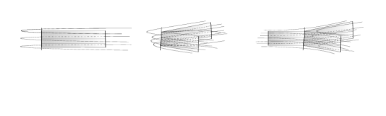
Figure 23. Behavior of ${\mathcal{F}}_{2}(\alpha)$ in the neighborhood of a partially umbilic curve  D${}_{1},$ D₂ and D${}_{3}.$

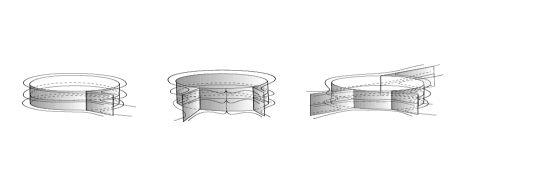
Figure 24. Behavior of ${\mathcal{F}}_{2}(\alpha)$ near the projective line (blowing-up).

In Fig. 25 it is shown the generic behavior of principal foliation ${\mathcal{F}}_{2}(\alpha)$ and ${\mathcal{F}}_{3}(\alpha)$ near the transitions of arcs D₁-D₂ and D₂-D₃. See [13, 14].

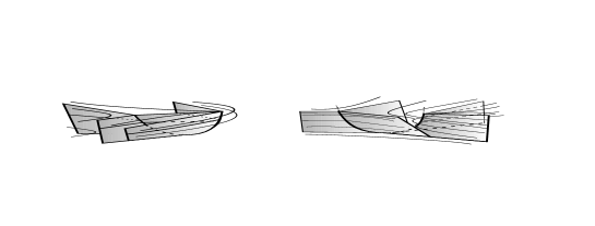
Figure 25. Behavior of ${\mathcal{F}}_{2}(\alpha)$ near a transition D₁-D₂ and of ${\mathcal{F}}_{2}(\alpha)$ and ${\mathcal{F}}_{3}(\alpha)$ near a transition D₂-D${}_{3}.$

10.2. Curvature lines near hyperbolic principal cycles

Next it will be described the behavior of principal foliations near principal cycles, i.e., closed principal lines of ${\mathcal{F}}_{i}(\alpha)$.

Let $c$ be principal cycle of the principal foliation ${\mathcal{F}}_{1}(\alpha)$.

With respect to the positive orthonormal frame $\{e_{1},e_{2},e_{3},N\},$ Darboux’s equations for the curve $\alpha\circ c$ are given by the following system, see [77].

$$\left(\begin{matrix}e_{1}^{\prime}\\ e_{2}^{\prime}\\ e_{3}^{\prime}\\ N^{\prime}\end{matrix}\right) =\left(\begin{matrix}0&\omega_{12}&\omega_{13}&k_{1}\\ -\omega_{12}&0&\omega_{23}&0\\ -\omega_{13}&-\omega_{23}&0&0\\ -k_{1}&0&0&0\end{matrix}\right)\left(\begin{matrix}e_{1}\\ e_{2}\\ e_{3}\\ N\end{matrix}\right)$$

where $\omega_{ij}=<\nabla_{e_{1}}e_{i},e_{j}>.$

In order to study the behavior of ${\mathcal{F}}_{1}(\alpha)$ in the neighborhood of $c$ we will study the Poincaré map $\Pi$ associated to ${\mathcal{F}}_{1}(\alpha)$ whose definition is reviewed as follows.

Let $(u_{1},u_{2},u_{3})$ be the system of coordinates given by lemma 1. Consider in these coordinates the transversal sections $\quad\{u_{1}=0\}$ and $\{u_{1}=L\}\quad$ and define the map $\Pi:\{u_{1}=0\}\rightarrow\{u_{1}=L\}$ in the following way.

Suppose $c$ be oriented by the parametrization $u_{1}$ and let $(u_{1},u_{2},u_{3})$ the solution of the differential equation that defines the principal line field ${\mathcal{L}}_{1}(\alpha)$, with initial condition $(u_{1},u_{2},u_{3})(0,u^{0}_{2},u^{0}_{3})=(0,u^{0}_{2},u^{0}_{3})$. So the Poincaré map is defined by

$$\Pi(u^{0}_{2},u^{0}_{3})=(u_{2}\scriptstyle(L,u^{0}_{2},u^{0}_{3})\displaystyle,u_{3}\scriptstyle(L,u^{0}_{2},u^{0}_{3})\displaystyle).$$

The principal cycle $c$ is called hyperbolic if the eigenvalues of $\Pi^{\prime}(0)$ are disjoint from the unitary circle, [72].

Proposition 10.

In the conditions above we have that the derivative of the Poincaré map $\Pi$ is given by $\Pi^{\prime}(0)=U(L)$, where $U$ is the solution of the following differential equation:

$$\left\{\begin{matrix}U^{\prime}&=AU\qquad\qquad\qquad\qquad\quad\\ U(0)&=I,\,A(u_{1})=A(u_{1}+L),\end{matrix}\right.\;A(u_{1}) =\left(\begin{matrix}\dfrac{\scriptstyle-k_{2}^{\prime}\displaystyle}{\scriptstyle(k_{2}-k_{1})\displaystyle}&\dfrac{\scriptstyle\omega_{23}(k_{3}-k_{1})\displaystyle}{\scriptstyle(k_{2}-k_{1})\displaystyle}\cr\dfrac{\scriptstyle-\omega_{23}(k_{2}-k_{1})\displaystyle}{\scriptstyle(k_{3}-k_{1})\displaystyle}&\dfrac{\scriptstyle-k_{3}^{\prime}\displaystyle}{\scriptstyle(k_{3}-k_{1})\displaystyle}\end{matrix}\right).$$

Theorem 15.

[15] Let $c$ be a principal cycle of ${\mathcal{F}}_{1}(\alpha).$ Suppose that the principal curvature $k_{1}$ is not constant along $c$. Then, given $\epsilon>0$, there exists an immersion $\tilde{\alpha}\in{\mathcal{J}}^{\infty,r}(\mathbb{\mathbb{missing}}M^{3},\mathbb{R}^{4})$ such that $||\alpha-\tilde{\alpha}||<\epsilon$ and $c$ is a hyperbolic principal cycle of ${\mathcal{F}}_{1}(\tilde{\alpha}).$

Remark 11.

Global aspects of principal lines of immersed hypersurfaces in $\mathbb{R}^{4}$ was studied in [13].

11. Concluding Comments

In this work an effort has been made to present most of the developments addressed to improve the local and global understanding of the structure of principal curvature lines on surfaces and related geometric objects. The emphasis has been put on those developments derived from the assimilation of ideas coming from the QTDE and Dynamical Systems into the classical knowledge on the subject, as presented in prestigious treatises such as Darboux [6], Eisenhart [9], Struik [78], Hopf [55], Spivak [77].

The starting point for the results surveyed here can be found in the papers of Gutierrez and Sotomayor [43, 44, 48], as suggested in the historical essay contained in sections 2.1 to 2.3.

The authors acknowledge the influence they received from the well established theories of Structural Stability and Bifurcations which developed from the inspiring classical works of Andronov, Pontrjagin, Leontovich [1] and Peixoto [63, 64]. Also the results on bifurcations of principal configurations outlined in [45] and further elaborated along this work are motivated in Sotomayor [71].

The vitality of the QTDE and Dynamical Systems, with their remarkable present day achievements, may lead to the belief that the possibilities for directions of future research in connection with the differential equations of lines of curvature and other equations of Classical Geometry are too wide and undefined and that the source of problems in the subject consists mainly in establishing an analogy with one in the above mentioned fields.

While this may partially true in the present work, History shows us that the consideration of problems derived from purely geometrical sources and from other fields such as Control Theory, Elasticity, Image Recognition and Geometric Optics, have also a crucial role to play in determining the directions for relevant research in our subject. In fact, at the very beginning, the works of Monge and Dupin and, in relatively recent times, also the famous Carathéodory Conjecture [17], [39], [50], [51, 52, 53], [56], [59], [61, 62], [68], [69, 70], [83], represent geometric sources of research directions leading to clarify the structure of lines of curvature and their umbilic singularities.

Acknowledgement.  The authors are grateful to L. F. Mello and C. Gutierrez for helpful remarks. Sotomayor thanks the hospitality of the Mathematics Department at Brown University, where part of this work was done.

Jorge Sotomayor
Instituto de Matemática e Estatística,
Universidade de São Paulo,
Rua do Matão 1010, Cidade Universitária,
CEP 05508-090, São Paulo, S.P., Brazil

Ronaldo Garcia
Instituto de Matemática e Estatística,
Universidade Federal de Goiás,
CEP 74001-970, Caixa Postal 131,
Goiânia, GO, Brazil

References

- [1] A. Andronov, E. Leontovich et al, Theory of Bifurcations of Dynamic Systems on a Plane, Jerusalem, Israel Program of Scientific Translations, (1973).
- [2] A. C. Asperti, Some Generic Properties of Riemannian Immersions, Bol. Soc. Bras. Mat. 11, (1978), pp. 191-216.
- [3] F. E. Browder, Editor, The mathematical heritage of Henri Poincaré, Proceedings of Symposia in Pure Mathematics, 39. American Mathematical Society, Parts 1 and 2. Providence, RI, (1983).
- [4] B. Bruce and D. Fidal, On binary differential equations and umbilic points, Proc. Royal Soc. Edinburgh 111A, (1989), pp. 147-168.
- [5] C. Carathéodory, Einfach Bemerkungen uber Nabelpunktscurven. Lecture at Breslau, Complete Works, 5, (1935), pp. 26-30.
- [6] G. Darboux, Leçons sur la Théorie des Surfaces, vol. IV. Sur la forme des lignes de courbure dans la voisinage d’un ombilic, Note 07, Paris: Gauthier Villars, (1896).
- [7] C. Dupin, Développements de Géométrie, Paris, (1813). Troisième Mémoire, art. IV et V, p. 157 et suiv.
- [8] L. Euler, Recherches sur la courbure des surfaces, Mémoires de l´Academie de Sciences de Berlin, 16, (1767), pp. 119-143, Opera Omnia: Series 1, Volume 28, (1955), pp. 1 - 22.
- [9] L. P. Eisenhart, A Treatise on Differential Geometry of Curves and Surfaces, Dover Publications, Inc., (1950).
- [10] G. Fischer, Mathematical Models, Vieweg, (1986).
- [11] V. T. Fomenko, Some Properties of Two-Dimensional Surfaces with zero Normal Torsion in , Math. USSR. Sbornik, 35, (1979), pp. 251-265.
- [12] A. R. Forsyth, Geometry of Four Dimensions, vols. I and II, Cambridge Univ. Press, (1930).
- [13] R. Garcia, Linhas de Curvatura de Hipersuperfícies Imersas no espaço , Pré-Publicação-IMPA, (Thesis), Série F, 27, (1989).
- [14] R. Garcia, Lignes de Courbure d’Hypersurfaces Immergées dans l’Espace , Anais Acad. Bras. Ciências, 64, (1992), pp. 01-06.
- [15] R. Garcia, Hyperbolic Principal Cycles on Hypersurfaces in , Annals of Global Analysis and Geometry, 11, (1993), pp. 185-196.
- [16] R. Garcia, Principal Curvature Lines near Partially Umbilic Points in hypersurfaces immersed in , Comp. and Appl. Math., 20, (2001), pp. 121–148.
- [17] R. Garcia and C. Gutierrez, Ovaloids of and their umbilics: a differential equation approach, J. Differential Equations, 168, (2000), no. 1, pp. 200–211.
- [18] R. Garcia, C. Gutierrez and J. Sotomayor, Structural Stability of asymptotic lines on surfaces immersed in , Bulletin de Sciences Mathematiques, 123, (1999), pp. 599-622.
- [19] R. Garcia, C. Gutierrez andJ. Sotomayor, Lines of Principal Curvature around umbilics and Whitney Umbrella Singularities, Tôhoku Mathematical Journal, 52, (2000), pp. 163-172.
- [20] R. Garcia, C. Gutierrez and J. Sotomayor, Bifurcations of Umbilic Points and Related Principal Cycles, Journ. Dyn. and Diff. Eq. 16, (2004), pp. 321-346.
- [21] R. Garcia, J. Llibre and J. Sotomayor, Lines of Principal Curvature on Canal Surfaces in , Anais da Acad. Brasileira de Ciências, 78, (2006), pp. 405-415.
- [22] R. Garcia, L. F. Mello and J. Sotomayor, Principal mean curvature foliations on surfaces immersed in . EQUADIFF 2003, pp. 939–950, World Sci. Publ., Hackensack, NJ, (2005).
- [23] R. Garcia and F. Sánchez-Bringas, Closed principal lines of surfaces immersed in the Euclidean 4-space, J. Dynam. Control Systems, 8, (2002), pp. 153–166.
- [24] R. Garcia and J. Sotomayor, Lines of curvature near principal cycles, Annals of Global Analysis and Geometry, 10, (1992), pp. 275-289.
- [25] R. Garcia and J. Sotomayor, Lines of Curvature near Singular Points of Implicit Surfaces, Bull.Sc. Math., 117, (1993), pp. 313-331.
- [26] R. Garcia and J. Sotomayor, Lines of curvature near hyperbolic principal cycles, Pitman Res.Notes, 285, (1993), pp. 255-262.
- [27] R. Garcia and J. Sotomayor, Lines of Curvature on Algebraic Surfaces, Bull. Sciences Math., 120, (1996), pp. 367-395.
- [28] R. Garcia and J. Sotomayor, Structural Stability of Parabolic Points and Periodic Asymptotic Lines, Matemática Contemporânea, 12, (1997), pp. 83-102.
- [29] R. Garcia and J. Sotomayor, Lines of axial curvature on surfaces immersed in , Differential Geom. Appl., 12, (2000), pp. 253–269.
- [30] R. Garcia and J. Sotomayor, Structurally stable configurations of lines of mean curvature and umbilic points on surfaces immersed in , Publ. Matemátiques, 45, (2001), pp. 431-466.
- [31] R. Garcia and J. Sotomayor, Lines of Geometric Mean Curvature on surfaces immersed in , Annales de la Faculté des Sciences de Toulouse, 11, (2002), pp. 377-401.
- [32] R. Garcia and J. Sotomayor, Lines of Harmonic Mean Curvature on surfaces immersed in , Bull. Bras. Math. Soc., 34, (2003), pp. 303-331.
- [33] R. Garcia and J. Sotomayor, Lines of Mean Curvature on surfaces immersed in , Qualit. Theory of Dyn. Syst., 5, (2004), pp. 137-183.
- [34] R. Garcia and J. Sotomayor, On the patterns of principal curvature lines around a curve of umbilic points, Anais da Acad. Brasileira de Ciências, 77, (2005), pp. 13-24.
- [35] R. Garcia and J. Sotomayor, Lines of Principal Curvature near Singular End Points of Surfaces in . Advanced Studies in Pure Mathematics, 43, (2006), pp. 437-462.
- [36] R. Garcia and J. Sotomayor, Umbilic points of codimension two. Discrete and Continuous Dynamical Systems, Series A, 17, (2007), pp. 293-308.
- [37] M. Golubitsky and D. Schaeffer, Singularities and Groups in Bifurcation Theory, vol.1, Springer Verlag, Applied Math. Sciences, 51, (1985).
- [38] A. Gullstrand, Zur Kenntniss der Kreispunkte, Ac. Math., 29, (1905), pp. 59-100.
- [39] C. Gutierrez, F. Mercuri and F. Sánchez-Bringas, On a conjecture of Carathéodory: Analyticity versus Smoothness, Experimental Mathematics, 5, (1996), pp. 33-37.
- [40] V. Guiñez and C. Gutierrez, Simple Umbilic points on surfaces immersed in , Discrete and Cont. Dyn. Systems, 9, (2003), pp. 877-900.
- [41] C. Gutierrez, I. Guadalupe, R. Tribuzy and V. Guíñez, Lines of Curvature on Surfaces Immersed in , Bol. Soc. Bras. Mat., 28, (1997), pp. 233-251.
- [42] C. Gutierrez, I. Guadalupe, J. Sotomayor and R. Tribuzy, Principal lines on Surfaces Minimally Immersed in Constantly Curved 4-Spaces, Dynamical Systems and Bifurcation Theory (Rio de Janeiro, 1985), Pitman Res. Notes Math. Ser., 160, Longman Sci. Tech., Harlow, (1987), pp. 91-120.
- [43] C. Gutierrez and J. Sotomayor, Structural Stable Configurations of Lines of Principal Curvature, Asterisque, 98-99, (1982), pp. 185-215.
- [44] C. Gutierrez and J. Sotomayor, An Approximation Theorem for Immersions with Structurally Stable Configurations of Lines of Principal Curvature, Lect. Notes in Math. 1007, (1983), pp. 332-368.
- [45] C. Gutierrez and J. Sotomayor, Lines of Curvature and Bifurcations of Umbilical Points, Colloquium on dynamical systems (Guanajuato, 1983), pp. 115–126, Aportaciones Mat. 05, Soc. Mat. Mexicana, México, (1985).
- [46] C. Gutierrez and J. Sotomayor, Closed Principal Lines and Bifurcations, Bol. Soc. Bras. Mat., 17 , (1986), pp. 1-19.
- [47] C. Gutierrez and J. Sotomayor, Principal Lines on Surfaces Immersed with Constant Mean Curvature, Trans. of Amer. Math. Society, 293 , (1986), pp. 751-766.
- [48] C. Gutierrez and J. Sotomayor, Lines of Curvature and Umbilic Points on Surfaces, Brazilian Math. Colloquium, Rio de Janeiro, IMPA, 1991. Reprinted as Structurally Configurations of Lines of Curvature and Umbilic Points on Surfaces, Lima, Monografias del IMCA, (1998).
- [49] C. Gutierrez and J. Sotomayor, Periodic lines of curvature bifurcating from Darbouxian umbilical connections, Springer Lect. Notes in Math., (1990), 1455, pp. 196–229.
- [50] C. Gutierrez and J. Sotomayor, Lines of Curvature, Umbilical Points and Carathéodory Conjecture, Resenhas IME-USP, 03, (1998), pp. 291-322.
- [51] H. Hamburger, Beweis einer Carathéodory Vermutung I, Ann. Math., 41, (1940), pp. 63-86.
- [52] H. Hamburger, Beweis einer Carathéodory Vermutung II, Acta. Math., 73, (1941), pp. 175-228.
- [53] H. Hamburger, Beweis einer Carathéodory Vermutung III, Acta. Math., 73, (1941), pp. 229-332.
- [54] D. Hilbert and S. Cohn Vossen, Geometry and the Imagination, Chelsea, (1952).
- [55] H. Hopf, Differential Geometry in the Large, Lectures Notes in Math., 1000, Springer Verlag, (1979).
- [56] V. V. Ivanov, An analytic conjecture of Carathéodory. Siberian Math. J. 43, no. 2, (2002), pp. 251–322.
- [57] J. A. Little, On Singularities of Submanifolds of higher Diemensional Euclidean Space, Ann. di Mat. Pura App., 83, (1969), pp. 261-335.
- [58] L. F. Mello, Mean directionally curved lines on surfaces immersed in , Publ. Mat. 47, (2003), pp. 415–440.
- [59] L. F. Mello and J. Sotomayor, A note on some developements on Carathéodory conjecture on umbilic points, Exposiciones Matematicae, 17, (1999), pp. 49-58.
- [60] G. Monge, Sur les lignes de courbure de la surface de l´Elipsoide, Journ. de l´Ecole Polytechnique II Cahier, (1796), pp. 145-165.
- [61] V. Ovskienko and T. Tabachnikov, Projective Differential Geometry Old and New, Cambridge University Press, (2005).
- [62] V. Ovskienko and T. Tabachnikov, Hyperbolic Carathéodory Conjecture, Proc. of Steklov Inst. of Mathematics, 258, (2007), pp. 178-193.
- [63] M. Peixoto, Structural Stability on two-dimensional manifolds, Topology, 1, (1962), pp. 101-120.
- [64] M. Peixoto, Qualitative theory of differential equations and structural stability, Symposium of Differential Equations and Dynamical Systems, J. Hale and J. P. La Salle, eds. N.Y., Acad. Press, (1967), pp. 469-480.
- [65] H. Poincaré, Mémoire sur les courbes définies par une équations différentielle, Journ. Math. Pures et Appl. 7, 1881, 375-422. This paper and its continuation, in 2 parts, are reprinted in Ouevres, Tome1, Paris: Gauthier-Villars, (1928).
- [66] C. Pugh, The Closing Lemma, Amer. Math. Journal 89, (1969), pp. 956-1009.
- [67] A. Ramírez-Galarza and F. Sánchez-Bringas, Lines of Curvature near Umbilical Points on Surfaces Immersed in . Annals of Global Analysis and Geometry, 13, (1995), pp. 129-140.
- [68] B. Smyth, The nature of elliptic sectors in the principal foliations of surface theory. EQUADIFF 2003, pp. 957–959, World Sci. Publ., Hackensack, NJ, (2005).
- [69] B. Smyth and F. Xavier, A sharp geometric estimate for the index of an umbilic on a smooth surface. Bull. London Math. Soc., 24, 1992, pp. 176–180.
- [70] B. Smyth and F. Xavier, Eigenvalue estimates and the index of Hessian fields. Bull. London Math. Soc., 33, (2001), pp. 109–112.
- [71] J. Sotomayor, Generic One Parameter Families of Vector Fields on two Dimensional Manifolds, Publ. Math. IHES, 43, (1974), pp. 5-46.
- [72] J. Sotomayor, Lições de Equações Diferenciais Ordinárias, Projeto Euclides, CNPq, IMPA, (1979).
- [73] J. Sotomayor, Closed lines of curvature on Weingarten immersions, Annals of Global Analysis and Geometry, 05, (1987), pp. 83-86.
- [74] J. Sotomayor, O Elipsóide de Monge, (Portuguese) Matemática Universitária, 15, (1993), pp. 33–47.
- [75] J. Sotomayor, El elipsoide de Monge y las líneas de curvatura, (Spanish) Materials Matemàtiques 2007 - 1, pp. 1–25, www.mat.uab.cat/matmat.
- [76] J. Sotomayor, Historical coments on Monge Ellipsoid and Lines of Curvature Mathematics ArXiv, (2003), http://front.math.ucdavies.edu/o411.5403.
- [77] M. Spivak, Introduction to Comprehensive Differential Geometry, Vol. III, IV, V Berkeley, Publish or Perish, (1980).
- [78] D. Struik, Lectures on Classical Differential Geometry, Addison Wesley Pub. Co., Reprinted by Dover Publications, Inc., (1988).
- [79] R. Taton, l’Oeuvre Scientifique de Monge, Presses Univ. de France, (1951).
- [80] E. Vessiot, Leçons de Géométrie Supérieure, Librarie Scientifique J. Hermann, Paris, (1919).
- [81] H. Whitney, The general type of singularity of a set of smooth functions of variables, Duke Math. J., 10, (1943), pp.161-172.
- [82] W. C. Wong, A new curvature theory for surfaces in euclidean 4-space, Comm. Math. Helv. 26, (1952), pp. 152-170.
- [83] F. Xavier, An index formula for Loewner vector fields, Math. Research Letters, 14, (2007), pp. 865-874.