Fundamental properties and applications of quasi-local black hole horizons

Abstract

The traditional description of black holes in terms of event horizons is inadequate for many physical applications, especially when studying black holes in non-stationary spacetimes. In these cases, it is often more useful to use the quasi-local notions of trapped and marginally trapped surfaces, which lead naturally to the framework of trapping, isolated, and dynamical horizons. This framework allows us to analyze diverse facets of black holes in a unified manner and to significantly generalize several results in black hole physics. It also leads to a number of applications in mathematical general relativity, numerical relativity, astrophysics, and quantum gravity. In this short review, I will discuss the basic ideas and recent developments in this framework, and summarize some of its applications with an emphasis on numerical relativity.

1 Introduction

The surface of a black hole has traditionally been defined using event horizons. Event horizons play a fundamental role in many seminal investigations in black hole physics. This includes Hawking’s area increase theorem, black hole thermodynamics, the uniqueness theorems, black hole perturbation theory and the topological censorship results. Moreover, the most important family of black holes for many purposes are the Kerr-Newman black holes. Similarly for almost all astrophysical purposes, most studies are carried our using Kerr black holes. Given this list of successful results and applications, is there any real need to go beyond event horizons and Kerr black holes?

There are indeed some situations where event horizons are not sufficient, and most of these have to do with the global nature of event horizons; we need to know the entire history of the spacetime in order to locate them. This leads to a practical problem for numerical relativity simulations. There is no way to locate event horizons using only Cauchy data at a given time without actually performing the simulation and constructing the full spacetime. Moreover, even after the event horizon is located, using it to calculate the physical parameters is fraught with difficulties. In particular, the Hamiltonian methods used to define the black hole parameters as generators of symmetries are not well adapted to the event horizon. All these problems are resolved in the case when the spacetime is stationary. However we would like to go beyond stationarity, and even for black holes in equilibrium, it should not be necessary to require the entire spacetime to be stationary.

One of the classic results of crucial importance to black holes which does not use event horizons are the singularity theorems of Penrose and Hawking [1, 2]. The presence of a closed trapped surface implies geodesic incompleteness in the future. The first singularity theorem was proved by Penrose in 1965 [1], and this paper also introduced the notion of a trapped surface. We shall use Penrose’s trapped surfaces to study black holes quasi-locally, without relying on global properties of the spacetime.

The rest of this review is organized as follows. Following a discussion of basic notions and definitions, we discuss the existence and non-uniqueness of quasi-local horizons, and the time evolution of marginally trapped surfaces in Sec. 2. Sec. 3 discusses the black hole area increase law. Finally Sec. 4 describes some applications in numerical relativity. The reader should beware that this is a biased review of quasi-local horizons with a focus on numerical relativity applications. There are a number of other interesting mathematical and physical aspects of quasi-local horizons which we shall not have time to discuss. The reader is referred to [3, 4, 5] for more complete reviews and references.

Trapped surfaces and the trapping region

The expansion of a congruence of null geodesics is defined as the rate of increase of an infinitesimal transverse 2-dimensional cross-section area $\delta A$ carried along with the geodesics:

$$\Theta=\frac{1}{\delta A}\frac{d\delta A}{dt}\,.$$ (1)

The definitions of the shear $\sigma_{ab}$ and twist $\omega_{ab}$ are also based on deformations of the cross-section. The particular geodesic congruence we consider are the ones orthogonal to a 2-surface $S$. Let us denote the in-going and out-going null normals to $S$ by $\ell^{a}$ and $n^{a}$ respectively, and let $\Theta_{(\ell)}$ and $\Theta_{(n)}$ be their respective expansions. For a sphere in flat space, the out-going light rays are diverging and the ingoing ones are converging, i.e. $\Theta_{(\ell)}>0$ and $\Theta_{(n)}<0$. $S$ is said to be a trapped surface if both sets of null-normals are converging: $\Theta_{(\ell)}<0$ and $\Theta_{(n)}<0$. A marginally trapped surface (MTS) is one for which $\Theta_{(\ell)}=0$ and $\Theta_{(n)}<0$. As shown by the singularity theorems, the presence of such surfaces is the signature of a spacetime containing a black hole. Note however that this is not necessarily a signature of strong gravitational field; they are present even for large black holes which have correspondingly small tidal forces at the horizon. It can be shown that trapped surfaces must lie inside the event horizon, and that cross-sections of the event horizon for stationary black holes are MTSs.

The spacetime region $\mathcal{T}$ containing trapped surfaces is called the trapped region. Similarly, if we restrict our attention to a initial-data surface $\Sigma$, and to trapped surfaces lying on $\Sigma$, we can similarly define the trapped region $\mathcal{T}_{\Sigma}\subset\Sigma$ which is, by definition, a subset of the full four-dimensional trapped region. An apparent horizon is the outermost MTS on $\Sigma$. It can be shown that the MTSs form the boundary of the trapped region on $\Sigma$. It seems plausible that the event horizon should be the boundary of $\mathcal{T}$. This is indeed the case in Schwarzschild where there exist spherically symmetric trapped surfaces all the way up to the event horizon, and the cross-section of the event horizon is a MTS. Thus, the event horizon separates the trapped and normal region of spacetime. This is also true for the Kerr black hole. However, in dynamical spacetimes, the event horizon is growing, and thus cross-sections of the event horizon have $\Theta_{\ell)}>0$. Thus, there cannot be a sequence of trapped surfaces which approach smoothly to the event horizon. Is it then still true that the event horizon is the boundary of the trapped region? It was proposed by Eardley that it is indeed the case [6], and that trapped surfaces can be deformed to get arbitrarily close to the event horizon (but the limit itself is not smooth). A useful toy example in spherical symmetry is the Vaidya spacetime which models the collapse of null dust. In this case, it is seen that the spherically symmetric trapped surfaces do not extend all the way to the event horizon. However, Eardley’s conjecture, if true, implies that there exist non-spherically symmetric trapped surfaces which extend up to the event horizons. Numerical evidence was provided in [7] and later proved analytically by Ben-Dov that this is indeed the case [8].

Figure 1: Conformal diagrams for (half of) Schwarzschild (left panel) and for the Vaidya spacetime (right panel). In Schwarzschild, there exist spherically symmetric MTSs all the way up to the event horizon. The shaded region in the right panel is flat Minkowski space. The collapse begins at a retarded time $v=0$ and forms a black hole. The analog of the Schwarzschild $r=2M$ surface is now spacelike and is denoted by $H$. Spherically symmetric MTSs cannot cross $H$.

Trapped surfaces form the basis of recent developments in the study of quasi-local horizons. One of the first papers which took trapped surfaces seriously was by Sean Hayward in 1994 who introduced the notion of a trapping horizon [9] which will be discussed later. Black holes in equilibrium were studied by Ashtekar, Beetle and Fairhurst [10, 11, 12] with the aim of using them in quantum gravity black hole entropy calculations [13]. They have been subsequently developed further and have been useful in other areas such as black hole mechanics [14, 15, 16, 17, 18, 19, 20, 21], numerical relativity, the study of hairy black holes (see e.g. [22, 23, 24, 25, 26]) etc.

2 Fundamental properties of black hole horizons

Let us outline some basic definitions and properties of quasi-local horizons. The starting point for most of these constructions is the notion of a marginally trapped tube (MTT) defined to be a three-surface of topology $S^{2}\times\mathbb{R}$ foliated by MTSs. It is useful to think of a MTT as being obtained by the time evolution of a MTS. The MTT is thus constructed by stacking up MTSs found at different times. The various kinds of quasi-local horizons are MTTs with additional conditions on whether it is a spacelike, timelike or null surface, and additional geometric requirements on $\Theta_{(n)}$.

Name	Signature	Additional conditions on $\Theta_{(n)}$ and $\Theta_{(\ell)}$
Isolated horizon	Null	None (but with additional conditions on other geometrical fields)
Dynamical horizon	Spacelike	$\Theta_{(n)}<0$
Timelike membrane	Timelike	None
Trapping horizon (future outer)	No restriction	$\Theta_{(n)}<0$ and $\mathcal{L}_{n}\Theta_{(\ell)}<0$

These various constructions are relevant in different circumstances. An isolated horizon models an isolated black hole in an otherwise dynamical spacetime. The event horizon of stationary black holes are isolated horizons. In a dynamical case, dynamical horizons or future-outer-trapping-horizons are the most relevant. Timelike membranes, as their name indicates, are timelike surfaces. Thus, they are not one-way membranes and do not function as valid black hole surfaces. They do however exist and can be found, for example, in numerical simulations of black hole mergers. Useful examples of these different types of horizons can be found in, e.g. [27, 28, 29].

The key applications of these notions have been in the black hole entropy calculations, in formulating a more general framework for black hole mechanics, in studying properties of hairy black holes with non-Abelian gauge fields or dilatons, and in helping to study mathematical properties of trapped surfaces. They have also been found to be useful in astrophysical context primarily through numerical simulations of black hole spacetimes.

The existence and non-uniqueness of quasi-local horizons

Let us now briefly discuss the time evolution of MTSs. Numerically, it is sometimes seen that apparent horizons behave discontinuously, and this is perhaps the main reason why they have not been taken seriously in the past. However, it turns out that the behavior of MTSs themselves is smooth; there is, to my knowledge, no known example when this is not the case. The discontinuous time evolution of apparent horizons is an artifact of the “outermost” condition appearing in the definition of an apparent horizon. There is now in fact a rigorous mathematical proof by Andersson, Mars and Simon that MTSs subject to a stability requirement (which is expected to hold for the physically most important cases) evolve smoothly [30, 31] (see also [32]). We briefly sketch the statement of the result.

An MTS $S$ on a spatial slice $\Sigma$ is said to be strictly-stably-outermost if there exists an infinitesimal first order outward deformation which makes $S$ strictly untrapped. Explicitly, if $\mathbf{r}$ is the unit spacelike normal to $S$ on $\Sigma$, then we consider displacements of $S$ (and geometric fields on $S$) along $f\mathbf{r}$ for some function $f$; outward deformations have $f\geq 0$. Then $S$ is strictly-stably-outermost if the first order variation of the expansion $\Theta_{(\ell)}$ is positive: $\delta_{f\mathbf{r}}\Theta_{(\ell)}>0$ for $f\geq 0$. A crucial tool in these results is the stability operator $L_{\mathbf{r}}[f]:=\delta_{f\mathbf{r}}\Theta_{(\ell)}$ which turns out to be an elliptic operator, and the stability condition can be recast as a condition on the principal eigenvalue of $L$; see also If this stability condition is satisfied, then the MTT produced by the time evolution of $S$ exists at least for a sufficiently short duration, and it continues to exist as long as this stability condition holds. Furthermore, the MTT in the neighborhood of $S$ is either null or spacelike. It is spacelike of the matter flux $T_{ab}\ell^{a}\ell^{b}$ is non-vanishing somewhere on $S$. The elliptic nature of $L$ ensures that the MTT is spacelike everywhere in a neighborhood of $S$ if the flux $T_{ab}\ell^{a}\ell^{b}$ is non-zero even in a very small region on $S$. It should be emphasized that these results do not imply that the time development of $S$ is unique. It in fact implies quite the opposite: for every choice of time evolution by a foliation by spacelike surfaces (i.e. for every choice of lapse and shift functions) there exists an MTT and the different MTTs constructed from the different gauge choices are, in general, distinct from each other. It is also worth noting that not all MTSs will satisfy the stability condition; the unstable MTSs will be inner horizons and actually occur quite frequently in numerical simulations [28] (though they are usually not looked for). However, even the unstable MTSs always seem to evolve smoothly as far as the numerical simulations are concerned. This leads us to believe that the existence result might be of more general validity and it might be possible to extend the above techniques to prove this. See [33, 34, 35] for further results on trapped surfaces and quasi-local horizons using similar techniques. See also [36] for interesting numerical results on the behavior of MTTs in binary black hole spacetimes.

Complementary to these existence results, there are other important results on dynamical horizons worth mentioning. In [37] it is proved that the foliation of a dynamical horizon $H$ by MTSs is unique. This, together with the existence results above implies that for a given MTSs on an initial slice $\Sigma$, the MTTs corresponding different time developments must really be distinct as 3-manifolds. There are also some restrictions on the location of the various dynamical horizons. For example, it is shown in [37] that for a given dynamical horizon $H$, there cannot be any closed MTSs (and thus no other DH) lying in the past domain of dependence of $H$. Thus, while DHs are far from unique, there are some restrictions on where they can occur. We briefly mention results regarding the (non-)existence of dynamical horizons in spacetimes with symmetries [37, 38, 39]. For example, it is shown in [38] that strictly stationary spacetime regions cannot contain trapped or marginally trapped surfaces, and thus no quasi-local horizons as well. Finally, a different approach to studying dyamical horizons is presented in [40] which considers the conditions on the Cauchy data on $H$ that must be satisfied if $H$ is a dynamical horizon. This can be studied in spherical symmetry, and it leads to necessary conditions for the spacetime to contain a dynamical horizon; in this regard, see also [41].

3 The second law

In this section, we outline the second law for dynamical/trapping horizons and its ramifications. But before doing so, it is worth mentioning the significant amount of work devoted to understanding the first law for quasi-local horizons. The fist law connects variations in the mass $M$ between two nearby black hole solutions to the surface gravity $\kappa$, area $A$, angular velocity $\Omega$ and angular momentum $J$ (the presence of other conserved charges is easy to incorporate):

$$\delta M=\frac{\kappa}{8\pi G}\delta A+\Omega\delta J\,.$$ (2)

This was initially proved for stationary Kerr black holes. It has been generalized to isolated horizons [15]. This is a significant generalization and it leads to a better understanding of the nature of the first law. It has since also been further extended to include a physical process version for dynamical horizons. There is also an earlier treatment by Hayward based on a different formulation.

Let us now turn to the second law. It was originally formulated by Hawking as: if matter satisfies the null energy condition, then the area of an event horizon can never decrease, i.e. $\Delta A\geq 0$. This is an exact result in full general relativity without any approximations. It suggests the identification of black hole area with entropy, and this identification has been very important as a driving force for progress in quantum gravity.

Classically, the second law leads to the picture of a black hole growing inexorably as it swallows matter and radiation. We can thus ask whether it is possible to get an equation like

$$\Delta A=\textrm{flux of matter + radiation}\,.$$ (3)

We require the fluxed to be quasi-local, geometric, and positive definite. The approach of Hartle and Hawking using perturbation theory and event horizons is a significant step, and it reinforces the possibility of the general validity of such a formula. It is easy to see however that if we restrict ourselves to event horizons, it is impossible to obtain in full generality because of, again, the global nature of the event horizon. A simple example is the Vaidya spacetime; in the shaded region before the null-radiation has formed the black hole, the event horizon is growing in anticipation of the black hole forming in the future. Thus, the event horizon is growing in flat space when surely any reasonable definition of the fluxes must be zero.

This non-locality can be seen in a different way. We can ask whether it is possible to obtain a differential equation for the rate of area increase. Working in the membrane paradigm, for event horizons, it was shown by Damour that

$$\frac{d^{2}A}{dt^{2}}-\kappa\frac{dA}{dt}=\ldots\qquad\textrm{with}\qquad\kappa>0\,.$$ (4)

The right hand side of this equation contains the source terms from the infalling matter/radiation which causes the black hole to grow, and all terms in thus equation are quasi-local. The sign of $\kappa$ is however a problem; it will generically lead to an exponential divergence if we attempt to solve (4) as an initial value problem. In fact, we need to impose $dA/dt\rightarrow 0$ as $t\rightarrow\infty$ to get finite solutions.

Can we reformulate the second law for quasi-local horizons? In fact, $\Delta A>0$ is a simple consequence of $\Theta_{(\ell)}=0$ and $\Theta_{(n)}<0$ for dynamical horizons. We can do better. Performing the decomposition of all geometric fields on a dynamical horizon, and using the constraint equations on a dynamical horizon, it can be shown that

$$\frac{R_{2}}{2G}-\frac{R_{1}}{2G}=\mathcal{F}^{(R)}_{m}+\mathcal{F}^{(R)}_{g}$$ (5)

where

$$\mathcal{F}^{(R)}_{g}:=\frac{1}{16\pi G}\int_{\Delta H}N_{R}\left\{|\sigma|^{2}+2|\zeta|^{2}\right\}\,d^{3}V$$ (6)

is the flux of the infalling gravitational radiation. The flux $\mathcal{F}^{(R)}_{g}$ has a number of reasonable properties. All terms appearing in the integral are local and coordinate independent, it is manifestly non-negative and it vanishes in spherical symmetry.

It is also possible to formulate a differential law for the area increase. Using a different component of the Einstein equation than what was used to get (5), Gourgoulhon and Jaramillo [42] obtained an equation of the following form:

$$\frac{d^{2}A}{dt^{2}}+\kappa^{\prime}\frac{dA}{dt}=\ldots\qquad\textrm{with}\qquad\kappa^{\prime}>0\,.$$ (7)

This is similar to (4), all terms in it are local and again the right hand side contains the source terms corresponding to infalling matter/radiation fluxes. However, the $dA/dt$ term now appears with the opposite sign, and we can therefore indeed solve this differential as an initial value problem by specifying $A$ and $dA/dt$ at some initial time $t=0$. The solution at some $t$ depends only on the fields at earlier times, and there is thus no teleological problem. This approach also solves other problems with the membrane paradigm. For example, the bulk viscosity of the horizon becomes positive [43, 42] as for a general fluid. Thus, consistent with the membrane paradigm, a black hole horizon can indeed be treated as a normal object and we can assign physical properties to it.

4 Applications in numerical relativity

Marginally trapped surfaces have been used in numerical simulations of black hole spacetimes almost from the very beginning of the field. This is because it is important to keep track of the black hole(s) while the simulation is in progress. The global nature of event horizons makes them not very useful for this purpose because, as discussed earlier, we need the full spacetime to locate the event horizon; the spacetime is the end product of the simulation, and is not available to us in real-time while the simulation is in progress. Thus, it is clear that quasi-local horizons can be useful in numerical relativity. They have so far been primarily used to extract gauge invariant information about the black hole such as its mass, angular momentum etc., and this is what we shall mostly focus on in this section. However, there are also other important applications which we will not be able to discuss. This includes the construction of initial data with trapped and marginally trapped surfaces as the inner boundary [44, 45, 46, 47, 48, 49], and the possibility of using fully constrained evolution schemes with a dynamical horizon as the inner boundary [50]. There has also been interest in clarifying the definition of surface gravity pf a quasi-local horizon, and the closely related notion of extremality [51, 52, 53]. This could prove to be useful for mathematical and astrophysical applications.

Mass and angular momentum

Numerical simulations are based on the initial value formulation of general relativity. Thus we are given an initial data set $(\Sigma,h_{ab},K_{ab})$ where $\Sigma$ is a 3-manifold embedded in the full spacetime, $h_{ab}$ a Riemannian metric on $\Sigma$, and $K_{ab}$ the second fundamental form describing how $\Sigma$ is embedded in the spacetime. Such an initial data set is evolved in time to construct the full spacetime. There are various formalisms for performing these evolutions and there are different choices of the variables that can be evolved, but these issues are not of much concern for our purposes. We instead pose a straightforward question. Assuming $\Sigma$ to be some slice of the Kerr spacetime, and assuming that $\Sigma$ intersects the event horizon in a complete sphere, how can we determine its parameters, i.e. its mass and angular momentum? Depending on the choice of $\Sigma$ and the choice of coordinates on $\Sigma$, the shape of the apparent horizon may turn out to be quite complicated. It may not seem axisymmetric and it may even be difficult to say whether we have a stationary black hole.

Let us reformulate this question in a much more general context. Consider a quasi-local horizon $H$ (i.e. an isolated, dynamical or trapping horizon) and let us assume that $\Sigma$ intersects $H$ in a cross-section $S$ which is a marginally trapped surface. We assume that $\Sigma$ is an asymptotically flat slice with $S$ as its inner boundary (the generalization to multiple black holes, i.e. when $S$ consists of several disconnected components is straightforward). Let us assume that $H$ is axisymmetric, i.e. it has a rotational vector $\varphi^{a}$ which has closed orbits, vanishes at two points on each cross-section of the MTSs which foliate $H$, and which is a symmetry of the geometrical fields on $H$. In particular $\varphi^{a}$ is a symmetry of the two metric $q_{ab}$ on every cross-section $S$ of $H$. Note that we only asked for $\varphi^{a}$ to exist on $H$, and not in the full spacetime and not even in a neighborhood of $H$. It is then possible to associate an angular momentum $J^{(\varphi)}_{S}$ of the horizon. Just like in classical mechanics where conserved quantities are defined as generators of symmetries, this calculation is based on a Hamiltonian formalism. We calculate the generator of diffeomorphisms along a rotational vector field $\phi^{a}$ which coincides with $\varphi^{a}$ on $H$ and with an asymptotic rotational symmetry at infinity [14, 15, 16, 17, 18] (analogous calculations also work in 2+1 [19] and higher [20, 21] dimensions). It is then easy to identify the contribution of the horizon to the angular momentum, and it turns out to be given by a surface integral over $S$ [54]:

$$J_{S}^{(\varphi)}=\frac{1}{8\pi}\oint_{S}K_{ab}\varphi^{a}dS^{b}\,.$$ (8)

Note that this formula is analogous to the standard formula for the angular momentum at spatial infinity (which is in fact also found by the same Hamiltonian calculation).

For an isolated horizon, as expected, $J^{(\varphi)}_{S}$ turns out to be independent of $S$. In this case, it is also easy to show that every cross-section of $H$ is actually axisymmetric It is now clear how the angular momentum associated with $S$ should be calculated. Having located $S$ on $\Sigma$, we need to find the appropriate symmetry vector on $S$ and then calculate the surface integral (8). There are now a number of methods proposed for calculating $\varphi^{a}$ [54, 55, 56].

With this background, the answer to the question posed at the beginning of this section is clear. If $S$ is a cross-section of the Kerr horizon, then it is guaranteed to have an axial symmetry vector $\varphi^{a}$ which can then be used to calculate the angular momentum via (8). Then given the angular momentum, we can calculate the area of the horizon thereby identifying the Kerr solution uniquely.

Given the angular momentum and the horizon area $A_{S}$ (and the area radius $R_{S}=\sqrt{A_{S}/4\pi}$, the horizon mass $M_{S}^{(\varphi)}$ is

$$M_{S}^{(\varphi)}=\frac{1}{2R_{S}}\sqrt{R_{S}^{4}+4(J_{S}^{(\varphi)})^{2}}\,.$$ (9)

This will give the correct answer for Kerr, and it is in fact also the result of a Hamiltonian calculation in the more general case of an axisymmetric quasi-local horizon.

Apart from getting the magnitude of the spin, it is also possible to estimate the direction of the angular momentum vector. The basic idea is to use the poles of $\varphi^{a}$ to define the axis of rotation. While the poles themselves are well defined on a given quasi-local horizon, the procedure of assigning a vector is not as clear cut. For example, it is not clear how the spin direction thus obtained can be compared with the spin direction calculated at spatial infinity. Nevertheless, this method has been applied and preliminary results are promising [57].

Equation (8) is now being used fairly widely in numerical relativity, though there is possibly room for improvement in the calculation of the symmetry vector field $\varphi^{a}$ along the lines of [55], for having a better conceptual understanding of the meaning of $J_{S}^{(\varphi)}$ when $\varphi^{a}$ is only an approximate symmetry vector (which is invariably the case in numerical simulations), and also a better understanding of the spin direction which is important for astrophysical applications.

Higher multipole moments

Apart from calculating the angular momentum and mass, it turns out that it is also possible to meaningfully define the higher multipole moments of a quasi-local horizon, at least in the axi-symmetric case. This construction was first carried out by [58] for isolated horizons, and subsequently applied by [3, 28] to the general case of a dynamical horizon. The construction starts with a coordinate system built using the given axial vector $\varphi^{a}$. $\phi\in[0,2\pi)$ is affine parameter along $\varphi^{a}$ and $\zeta=\cos\theta$ defined by $d\zeta\propto\star\varphi$ (the proportionality factor is chosen by requiring $\oint_{S}\zeta d^{2}V=0$). Then we use the spherical harmonics in these $(\theta,\phi)$ coordinates to define the mass and current multipole moments:

$$M_{n}^{(\varphi)}=\frac{R_{S}^{n}M_{S}^{(\varphi)}}{8\pi}\oint_{S}\left\{\tilde{{R}}P_{n}(\zeta)\right\}d^{2}V\,,\quad J_{n}^{(\varphi)}=\frac{R_{S}^{n-1}}{8\pi}\oint_{S}P_{n}^{\prime}(\zeta)\bar{K}_{ab}\varphi^{a}d^{2}S^{b}$$ (10)

where $P_{n}$ is the $n^{\rm th}$ order Legendre polynomial and $P_{n}^{\prime}$ its derivative.

These equations provides the source multipole moments of black hole, which are in general distinct from the field multipole moments defined at infinity. For isolated horizons, it can be shown [58] that the intrinsic horizon geometry is completely characterized by these multipole moments, i.e. any two isolated horizons with the same multipole moments are diffeomorphic to each other. $J_{0}$ vanishes by absence of monopole (NUT) charges, $M_{0}$ is mass and $J_{1}$ is angular momentum. In Kerr, $M_{0}$ and $J_{1}$ determine all higher moments. In Schwarzschild, only $M_{0}\neq 0$. The higher moments provide a convenient way of quantifying the deviation from Kerr. These multipole moments were applied in some example numerical simulations in [28] where it was shown that the black holes do indeed converge to Kerr very quickly after merger. However, the simulations were unfortunately not accurate enough to extract the late time decay rates of the multipole moments which would be the analog of Price’s law for dynamical horizons. Hopefully this can be measured in the future using long duration accurate simulations.

Quasi-local linear momentum

The calculation of black hole linear momentum is of astrophysical importance in the context of the recoil velocity produced during the merger of two black holes. The reason for the recoil is the anisotropic emission of gravitational radiation. It has been found that certain initial spin configurations lead to a much larger than expected value of this recoil velocity and the largest contribution turns out to be from the merger phase. This result is especially interesting for the case of super-massive black holes; if the recoil is large enough, the remnant black hole may be kicked out of the host galaxy and this has important astrophysical implications. Most calculations of the recoil velocity are based on the gravitational waveform extracted far away from the black hole which measures the center-of-mass momentum of the system. It is thus natural to ask whether one can measure the momentum quasi-locally for the two individual black holes. This would be a useful consistency check and it could also give us more detailed information about the dynamics of the merger. The possibility of measuring the linear momentum, and more generally the quasi-local energy-momentum four-vector, is also of mathematical interest.

So far, we have justified the equations for angular momentum, mass and energy by Hamiltonian methods. For the angular momentum we assumed the existence of a rotational symmetry and for energy and mass we need to pick out a preferred time evolution vector field at the horizon. Following the same line of reasoning, one might think of defining linear momentum by assuming the existence of a translational symmetry in a neighborhood of the horizon, or at least some preferred translational vector field. While it might be possible to do this in special cases, for example when the data is conformally flat, it is clearly not something we can assume generally. Unlike for angular momentum where there are interesting regimes where approximate axisymmetry is a valid assumption, the basis for carrying over this approach to linear momentum is much less secure.

Let us then try a more heuristic approach. Just as the formula for horizon angular momentum is analogous to the angular momentum at spatial infinity, let us apply the formula for linear momentum at infinity to the horizon. At spatial infinity, for a given asymptotic translational Killing vector field $\xi^{a}$, the momentum is

$$P_{\xi}^{\rm ADM}=\frac{1}{8\pi}\oint_{S_{\infty}}(K_{ab}-Kh_{ab})\xi^{a}dS^{b}$$ (11)

where $S^{\infty}$ is the sphere at infinity. This motivates the following definition at the horizon:

$$P_{\xi}^{(S)}=\frac{1}{8\pi}\oint_{S}(K_{ab}-Kh_{ab})\xi^{a}dS^{b}$$ (12)

where $\xi^{a}$ is some translational vector at the horizon. Using the constraint equations of $\Sigma$, it is easy to show

$$P_{\xi}^{\rm ADM}-P_{\xi}^{(S)}=\frac{1}{16\pi}\int(K^{ab}-K\gamma^{ab})\mathcal{L}_{\xi}h_{ab}d^{3}V\,.$$ (13)

The right hand side vanishes in some special cases, e.g. when $\xi^{a}$ is a conformal Killing vector on $\Sigma$, and the data is maximal ($K=0$). We also take $\xi^{a}$ to be coordinate basis vectors to get the three components of linear momentum. This definition is clearly gauge dependent, but it does seem sufficiently worthwhile to try it out in a numerical simulation. This was done in [59], and the preliminary results are encouraging.

An example result is shown in fig. 2 for a head on collision of two black holes with equal masses, and spins orthogonal to the line joining the two black holes and oppositely aligned with magnitude $0.15M^{2}$. The remnant black hole is non-spinning and the expected recoil velocity is $20.4\,$km/s. Figure 2 shows the result of applying (12) at different resolutions. The extrapolated result turns out to be $21.5\,$km/s which is in fairly good agreement with the calculation at infinity.

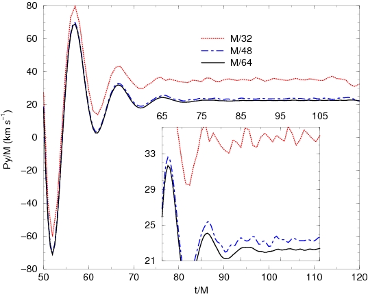
Figure 2: Linear momentum of the remnant black hole produced by the headon merger of black holes with anti-aligned spins for different resolutions.

5 Conclusions

In this talk we have outlined some properties of quasi-local horizons with applications to numerical relativity. We have seen that marginally trapped surfaces are not as badly behaved as one might have thought based on intuition about apparent horizons. It is possible to prove useful and interesting mathematical results about them and they can be used to study black hole physics. They have applications in diverse fields ranging from quantum gravity to numerical relativity. In numerical relativity we have shown how one can extract physical parameters of black holes such as its mass, angular momentum and the higher source multipole moments as well. We have also discussed preliminary ideas about the quasi-local linear momentum of black holes which could be of some astrophysical importance. On a more general note, we have seen that numerical relativity can be used as a tool for proposing and testing mathematical conjectures regarding trapped surfaces and black holes and in fact more generally problems in geometric analysis which are difficult to deal with analytically.

Bibliography

Bibliography

- [1] Roger Penrose. Gravitational collapse and space-time singularities. Phys. Rev. Lett., 14:57–59, 1965.
- [2] S. W. Hawking and R. Penrose. The singularities of gravitational collapse and cosmology. Proc. Roy. Soc. Lond., A314:529–548, 1970.
- [3] Abhay Ashtekar and Badri Krishnan. Isolated and dynamical horizons and their applications. Living Rev. Rel., 7:10, 2004.
- [4] Eric Gourgoulhon and Jose Luis Jaramillo. A 3+1 perspective on null hypersurfaces and isolated horizons. Phys. Rept., 423:159, 2006.
- [5] Ivan Booth. Black hole boundaries. Can. J. Phys., 83:1073–1099, 2005.
- [6] D.M. Eardley. Black hole boundary conditions and coordinate conditions. Phys. Rev. D, 57:2299–2304, 1998.
- [7] Erik Schnetter and Badri Krishnan. Non-symmetric trapped surfaces in the schwarzschild and vaidya spacetimes. Phys. Rev., D73:021502, 2006.
- [8] Ishai Ben-Dov. Outer trapped surfaces in vaidya spacetimes. Phys. Rev., D75:064007, 2007.
- [9] S.A. Hayward. General laws of black hole dynamics. Phys. Rev. D, 49:6467–6474, 1994.
- [10] A. Ashtekar, C. Beetle, and S. Fairhurst. Isolated horizons: a generalization of black hole mechanics. Class. Quantum Grav., 16:L1–L7, 1999.
- [11] A. Ashtekar, C. Beetle, and S. Fairhurst. Mechanics of isolated horizons. Class. Quantum Grav., 17:253–298, 2000.
- [12] A. Ashtekar, C. Beetle, O. Dreyer, S. Fairhurst, B. Krishnan, J. Lewandowski, and J. Wisniewski. Generic isolated horizons and their applications. Phys. Rev. Lett., 85:3564–3567, 2000.
- [13] A. Ashtekar, J.C. Baez, and K.V. Krasnov. Quantum geometry of isolated horizons and black hole entropy. Adv. Theor. Math. Phys., 4:1–94, 2000.
- [14] A. Ashtekar, C. Beetle, and J. Lewandowski. Mechanics of rotating isolated horizons. Phys. Rev. D, 64:1–17, 2001.
- [15] A. Ashtekar, S. Fairhurst, and B. Krishnan. Isolated horizons: Hamiltonian evolution and the first law. Phys. Rev. D, 62:1–29, 2000.
- [16] I.S. Booth. Metric-based hamiltonians, null boundaries and isolated horizons. Class. Quantum Grav., 18:4239–4264, 2001.
- [17] Ivan Booth and Stephen Fairhurst. Horizon energy and angular momentum from a hamiltonian perspective. Class. Quant. Grav., 22:4515–4550, 2005.
- [18] Ivan S. Booth. Metric-based hamiltonians, null boundaries, and isolated horizons. Class. Quant. Grav., 18:4239–4264, 2001.
- [19] A. Ashtekar, O. Dreyer, and J. Wisniewski. Isolated horizons in 2+1 gravity. Adv. Theor. Math. Phys., 6:507–555, 2002.
- [20] Mikolaj Korzynski, Jerzy Lewandowski, and Tomasz Pawlowski. Mechanics of multidimensional isolated horizons. Class. Quant. Grav., 22:2001–2016, 2005.
- [21] Tomas Liko and Ivan Booth. Isolated horizons in higher-dimensional einstein-gauss- bonnet gravity. Class. Quant. Grav., 24:3769, 2007.
- [22] A. Ashtekar and A. Corichi. Laws governing isolated horizons: Inclusion of dilaton coupling. Class. Quantum Grav., 17:1317–1332, 2000.
- [23] A. Ashtekar, A. Corichi, and D. Sudarsky. Hairy black holes, horizon mass and solitons. Class. Quantum Grav., 18:919–940, 2001.
- [24] A. Ashtekar, A. Corichi, and D. Sudarsky. Non-minimally coupled scalar fields and isolated horizons. Class. Quantum Grav., 20:3513–3425, 2003.
- [25] B. Kleihaus, J. Kunz, A. Sood, and M. Wirschins. Horizon properties of einstein–yang–mills black hole. Phys. Rev. D, 65:1–4, 2002.
- [26] B. Kleihaus and J. Kunz. Static black-hole solutions with axial symmetry. Phys. Rev. Lett., 79:1595–1598, 1997.
- [27] Ivan Booth, Lionel Brits, Jose A. Gonzalez, and Chris Van Den Broeck. Marginally trapped tubes and dynamical horizons. Class. Quant. Grav., 23:413–440, 2006.
- [28] Erik Schnetter, Badri Krishnan, and Florian Beyer. Introduction to dynamical horizons in numerical relativity. Phys. Rev., D74:024028, 2006.
- [29] Alex B. Nielsen and Matt Visser. Production and decay of evolving horizons. Class. Quant. Grav., 23:4637–4658, 2006.
- [30] Lars Andersson, Marc Mars, and Walter Simon. Stability of marginally outer trapped surfaces and existence of marginally outer trapped tubes. 2007.
- [31] Lars Andersson, Marc Mars, and Walter Simon. Local existence of dynamical and trapping horizons. Phys. Rev. Lett., 95:111102, 2005.
- [32] Ivan Booth and Stephen Fairhurst. Isolated, slowly evolving, and dynamical trapping horizons: geometry and mechanics from surface deformations. Phys. Rev., D75:084019, 2007.
- [33] Lars Andersson and Jan Metzger. Curvature estimates for stable marginally trapped surfaces. 2005.
- [34] Jan Metzger. Blowup of jang’s equation at outermost marginally trapped surfaces. 2007.
- [35] Lars Andersson and Jan Metzger. The area of horizons and the trapped region. 2007.
- [36] Bela Szilagyi, Denis Pollney, Luciano Rezzolla, Jonathan Thornburg, and Jeffrey Winicour. An explicit harmonic code for black-hole evolution using excision. Class. Quant. Grav., 24:S275–S293, 2007.
- [37] Abhay Ashtekar and Gregory J. Galloway. Some uniqueness results for dynamical horizons. Adv. Theor. Math. Phys., 9:1–30, 2005.
- [38] Marc Mars and Jose M. M. Senovilla. Trapped surfaces and symmetries. Class. Quant. Grav., 20:L293–L300, 2003.
- [39] Alberto Carrasco and Mars Mars. On marginally outer trapped surfaces in stationary and static spacetimes. 2007.
- [40] Robert Bartnik and James Isenberg. Spherically symmetric dynamical horizons. Class. Quant. Grav., 23:2559–2570, 2006.
- [41] Catherine Williams. Asymptotic behavior of spherically symmetric marginally trapped tubes. 2007.
- [42] Eric Gourgoulhon and Jose Luis Jaramillo. Area evolution, bulk viscosity and entropy principles for dynamical horizons. Phys. Rev., D74:087502, 2006.
- [43] Eric Gourgoulhon. A generalized damour-navier-stokes equation applied to trapping horizons. Phys. Rev., D72:104007, 2005.
- [44] J.L. Jaramillo, E. Gourgoulhon, and G.A. Mena Marugán. Inner boundary conditions for black hole initial data derived from isolated horizons, 2004.
- [45] S. Dain, J.L. Jaramillo, and B. Krishnan. On the existence of initial data containing isolated black holes, December 2004.
- [46] S. Dain. Trapped surfaces as boundaries for the constraint equations. Class. Quantum Grav., 21:555–574, 2004.
- [47] David Maxwell. Solutions of the einstein constraint equations with apparent horizon boundary. Commun. Math. Phys., 253:561–583, 2004.
- [48] Eric Gourgoulhon. Construction of initial data for 3+1 numerical relativity. 2007.
- [49] Brian Smith. Black hole initial data with a horizon of prescribed geometry. 2007.
- [50] Jose Luis Jaramillo, Eric Gourgoulhon, Isabel Cordero-Carrion, and Jose Maria Ibanez. Trapping horizons as inner boundary conditions for black hole spacetimes. 2007.
- [51] Ivan Booth. Two physical characteristics of numerical apparent horizons. 2007.
- [52] Ivan Booth and Stephen Fairhurst. Extremality conditions for isolated and dynamical horizons. 2007.
- [53] Alex B. Nielsen and Jong Hyuk Yoon. Dynamical surface gravity. 2007.
- [54] O. Dreyer, B. Krishnan, E. Schnetter, and D. Shoemaker. Introduction to isolated horizons in numerical relativity. Phys. Rev. D, 67:1–14, 2003.
- [55] Gregory B. Cook and Bernard F. Whiting. Approximate killing vectors on . Phys. Rev., D76:041501, 2007.
- [56] Mikolaj Korzynski. Quasi–local angular momentum of non–symmetric isolated and dynamical horizons from the conformal decomposition of the metric. 2007.
- [57] Manuela Campanelli, Carlos O. Lousto, Yosef Zlochower, Badri Krishnan, and David Merritt. Spin flips and precession in black-hole-binary mergers. Phys. Rev., D75:064030, 2007.
- [58] A. Ashtekar, J. Engle, T. Pawlowski, and C. Van Den Broeck. Multipole moments of isolated horizons. Class. Quantum Grav., 21:2549–2570, 2004.
- [59] Badri Krishnan, Carlos O. Lousto, and Yosef Zlochower. Quasi-local linear momentum in black-hole binaries. Phys. Rev., D76:081501, 2007.