Temperature Relaxation in Hot Dense Hydrogen

Abstract

Temperature equilibration of hydrogen is studied for conditions relevant to inertial confinement fusion. New molecular-dynamics simulations and results from quantum many-body theory are compared with Landau-Spitzer (LS) predictions for temperatures $T$ from 50 eV to 5000 eV, and densities with Wigner-Seitz radii $r_{s}=1.0$ and $0.5$. The relaxation is slower than the LS result, even for temperatures in the keV range, but converges to agreement in the high-$T$ limit.

Introduction – While a first-principles description of the equilibrium properties of strongly coupled Coulomb systems is a formidable task EOS , nonequilibrium systems pose an even greater challenge. Short-pulse lasers and shock waves create nonequilibrium states. Thus, Coulomb systems as diverse as warm dense matter Riley , ultracold plasmas Killian , shocked semiconductors Ng , and dense deuterium Knudsen can now be readily created in the laboratory, but initially under nonequilibrium conditions. Similarly, energy relaxation (ER) in astrophysical plasmas is important to the physics of fusion of H, C, etc., in determining stellar evolutiondeWitt . Here, we consider the ER of nonequilibrium dense hydrogen due to its importance in inertial confinement fusion (ICF)ICF .

The earliest theories of ER in plasmas were formulated by Landau Land and Spitzer Spit (denoted LS). The LS approach is applicable to dilute, hot, fully ionized plasms where the collisions are weak, binary, and involve negligible quantum effects; essentially, LS is Rutherford’s Coulomb scattering formula applied to a Maxwellian distribution. A characteristic feature of the LS approach is the use of a Coulomb logarithm (CL), i.e.,

$${\cal L}\equiv\ln\Lambda\sim\int_{b_{min}}^{b_{max}}\!db/b\sim\int_{k_{max}}^{k_{min}}\!dk/k$$ (1)

where $b_{min}$ (or $1/k_{max}$) and $b_{max}$ (or $1/k_{min}$) are suitable, but ad hoc, impact parameter (or momentum) cutoffs for the Coulomb collision. The full quantum mechanical method, based on calculating a transition rate, does not suffer from this problem. Calculations at the Fermi golden-rule level and beyond have been made by Dharma-wardana et al. DWP ; mwcd ; Hazak . Such methods automatically include degeneracy effects, effects of collective modes, and strong coupling. Other approaches employ convergent kinetic equations Gould_Dewitt ; GMS . Hansen and McDonald HM (denoted HM) and Reimann and Toepffer have directly obtained ER via molecular dynamics (MD) simulations.

In a hydrogen plasma the particle charges $z_{i},z_{j}$ are $\pm 1$, in atomic units, where the electronic charge $|e|$=$\hbar$=$m_{e}$=1. The mean electron and proton densities $n$ and $\rho$ are identical. The ratio of a typical Coulomb energy to the kinetic energy becomes, in the classical regime, $\Gamma=1/(r_{s}T)$, where $T$ is the temperature in energy units, and $\Gamma=r_{s}$ in the quantum regime. $r_{s}=\left[3/(4\pi n)\right]^{1/3}$ is the radius of the Wigner-Seitz sphere of an electron or a proton. The properties of partially degenerate fully-ionized plasmas require two independent parameters, e.g., both $r_{s}$ and $\theta=T/E_{F}$, where $E_{F}=\left(3\pi^{2}n\right)^{2/3}/2$ is the Fermi energy Murillo_tut . The LS analysis of ER is in terms of e-p collisions in a Maxwellian gas. Relative to the LS approach, some theoretical approaches relax faster GMS , or slower DWP ; Hazak . HM concluded that many-body effects are negligible and that the the LS result holdsHM . There is currently no direct experimental data for ER rates, although such experiments are under wayTaccetti ; GaretaRiley .

Here, we present larger HM-like molecular-dynamics (MD) simulations and quantum many-body calculations to narrow the gap in our predictions of ER rates for hot, dense hydrogen relevant to ICF targets composed of dense cryogenic fuel rapidly laser compressed to keV temperatures. The modeling of these dense plasmas covers physical processes over many orders of magnitude in density and temperature. Nonequilibrium quantum simulations require theoretical breakthroughs that are not yet fully established; however, the MD techniques that employs quantum-corrected effective potentials can be usefully applied to these problems. Since MD simulations attempt to solve the many-body equations of motion exactly, they are likely to provide accurate ER rates for hot, dense hydrogen.

Molecular dynamics.– Several issues arise in simulations of plasmas with temperatures in the $10^{2}$-10³ eV range. Because the screening length and mean-free-path are larger at higher temperatures, we have varied the number of particles widely (maximum of several thousand), with $N$=500 used for the results presented here. Also, because the ER time varies roughly as $T_{e}^{3/2}$, these simulations required millions of time steps for the higher-temperature cases. Compounding the longer runs was the need for much smaller time steps (as small as $0.005\omega_{pe}^{-1}$, where $\omega_{pe}$ is the usual electron plasma frequency), as a result of high velocity collisions at high temperature. Such issues are not unexpected, but have rarely been dealt with, since MD is typically applied to strongly coupled (i.e., cooler) classical systems. We carried out direct simulations of electrons and protons since the Born-Oppenheimer approximation is not applicable to this problem. The mass ratio ($1:1836$) was used due to our interest in mass-dependent collective mode effects. Finally, integrations were carried out with the velocity-Verlet algorithm using an ${\cal O}(N^{3/2})$ Ewald method.

The Coulomb interaction $1/r$ of classical physics is replaced by the mean-value of the operator $1/\hat{r}$ in quantum systems. This feature modifies the short-ranged behaviour of the electron-electron and electron-proton interactions, since the de Broglie wavelength of the electron is not negligible for small $r$. Also, unlike the classical electron-proton interaction which always leads to a bound state, the delocalized electron does not bind to the proton for regimes studied here. These effects are included in the e-e and e-p potentials by solving the relevant Schrodinger equations for the two-body scattering processes. These lead to diffraction-corrected Coulomb potentials $v_{ij}^{dfr}(r_{ij})$ which are Coulomb-like for distances larger than the respective de Broglie lengths, $\lambda_{ij}=1/\sqrt{2\pi\mu_{ij}T_{e}}$. Here $\mu_{ij}$ are the effective masses of the colliding pair. The choice of $b_{min}=\lambda_{ij}$ is usal in the LS approaches.

Then interaction $\phi_{ij}(r)$ between the pair $i,j$ is given by

$$\phi_{ij} = v_{ij}^{dfr}(r_{ij})+v_{ee}^{Pau}(r)$$ (2)

$$v_{ij}^{dfr}(r_{ij}) = \frac{z_{i}z_{j}}{r_{ij}}\left[1-e^{\left(-\frac{f_{ij}r_{ij}}{\lambda_{ij}}\right)}\right]+v^{Ewl}_{ij}(r_{ij})$$ (3)

where $v^{Ewl}_{ij}$ is the Ewald potential. The potential, $v_{ee}^{Pau}$, accounts for the spin-averaged Pauli exclusion between two electrons. This ensures that the “non-interacting” electron pair distribution function (PDF) calculated from a classical simulation is just the non-interacting quantum PDF Lado ; CHNC . The explicit formJonesMurillo used by HM is adequate for most of the range studied in this paper. The factor $f_{ij}$ is unity for all except the cross-species case $f_{ep}$. This is chosen using CHNC. The CHNC uses the above potentials and a classical fluid temperature $T_{cf}=\surd{T_{e}^{2}+T_{q}^{2}}$ where the quantum temperature $T_{q}$ is defined in Ref. CHNC . The $f_{ep}$ factor at a given $r_{s},\,T_{e},\,T_{p}$ is fixed by requiring that the CHNC $g_{ep}(r)$, at $r=0$ is the same as the Kohn-Sham value of $g_{ep}(r=0)$, as discussed more fully in Ref. DW-Murillo . The factors $f_{ep}$ are within 5% of unity for the conditions of our study.

To validate the potentials under two-temperature, dense-plasma conditions, we carried out (using $\phi_{ij}$ and its simplified HM forms) MD and CHNC for the conditions $r_{s}=1.0$, $T_{e}=50$eV, and $T_{i}=10$eV. In the MD, electron and proton velocity-scaling thermostats were used to create the two-temperature system, whereas recent results for the cross-species temperature $T_{ep}$ DW-Murillo were used in the CHNC. The pair distribution functions $g_{ij}(r)$ are shown in Fig. (1).

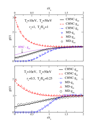
Figure 1: Pair distribution functions from MD (data points), CHNC (thick lines) for dense hydrogen, $r_{s}=0.5$ and 1, $T/E_{F}=$0.25 and 1. The $g_{ee}$ from a simple HNC calculation (i.e., no quantum temperature, no Pauli potential) with just $v_{ij}^{dfr}$ is also shown for $r_{s}=1$.

Temperature equilibration rates were determined for the two densities $r_{s}=0.5$ ($n_{e}=1.5\times 10^{25}$cm^-3) and $r_{s}=1.0$ ($n_{e}=1.61\times 10^{24}$cm^-3) over the temperature range $0.25<\theta<20$. In practice, an equilibration stage with separate electron and proton velocity-scaling thermostats was used to establish a two-temperature system. This was followed by a microcanonical evolution in which the temperatures were relaxed, with

$$T_{j}(t)=\frac{m_{j}}{3N_{j}}\sum_{i=1}^{N_{j}}v_{j}^{2}(t),$$ (4)

for each species $j$. Energy conservation was carefully monitored to assure stability at the elevated temperatures. Stability was quantified by $\Delta E=\frac{1}{N}\sum_{i=1}^{N}\left|\frac{E_{i}-E_{0}}{E_{0}}\right|$, where $E_{i}$ is the energy at the $i$-th timestep. The timestep was chosen by first performing several simulations with varying timesteps for temperatures $T=100,250,500,750$eV and noting the impact on $\Delta E$. As mentioned above, the timestep required for stability decreases dramatically with increasing temperature. A fit to the slope of the temperature profiles yielded the equilibration rate; in practice, the ion temperature was fixed for all runs at $T_{i}=10$eV so that the reported results are $\partial T_{e}/\partial t$. Over the range of temperatures considered, the relaxation rate should be very insensitive to the ion temperature.

Quantum transition rates.– The most transparent, strictly quantum approach to the calculation of the ER rate is to treat it as a transition rate where an electron in an initial momentum state $\vec{k}_{i}$ transfers to a final state $\vec{k}_{f}$, while a proton in the initial momentum eigenstate $\vec{p}_{i}$ absorbs energy and transfers to a final eigenstate $\vec{p}_{f}$. The availability of such states depends on the products of Fermi occupation factors $n_{k_{i}}(1-n_{k_{f}})$, and similarly for the proton states. The strength of the transition depends on the matrix element between the initial and final states. This matrix element may be taken in lowest-order theory (Born approximation) or in higher order (i.e, a $T$-matrix evaluation). These are the usual ingredients of the Fermi golden rule (FGR) for the transition rate. The summation over all such pair processes gives the total ER rate. But such summations immediately convert the description of the plasma into a description containing the full spectrum of single-particle and collective modes. The spectrum of all modes is given by the spectral function $A_{j}(q,\omega,T_{j})$ where the species index $j=e$ or $p$. These spectral functions are given by the imaginary parts of the corresponding dynamic response functions $\chi^{j}(\vec{k},\omega)$, e.g, Eq. (16) of Ref. Hazak . The ER rate evaluated within the Fermi golden rule, $R_{fgr}$ can be expressed in terms of the response functions of the plasma as follows, given in Eqs. (4)-(7) of Ref.mwcd , and Eq. (15) of Ref. Hazak :

$$R_{fgr} = \frac{dK}{dt}=\int\frac{d^{3}k}{\left(2\pi\right)^{3}}\frac{\omega d\omega}{2\pi}(\Delta B)F_{ep}$$ (5)

$$\Delta B = \coth(\omega/2T_{e})-\coth(\omega/2T_{p})$$ (6)

$$F_{ep} = |(V_{ep}(k)|^{2}\Im\left[\chi^{p}(\vec{k},\omega)\right]\Im\left[\chi^{e}\left(\vec{k},\omega\right)\right]$$ (7)

In the above we have used the spherical symmetry of the plasma to write scalars $q,k$ instead of $\vec{q},\,\vec{k}$ to simplify the notation.

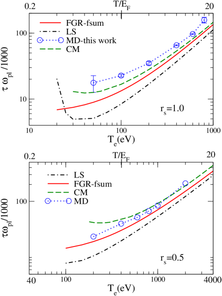
Figure 2: The relaxation time $\tau/1000$, in units of the inverse electon-plasma frequency, for dense hydrogen, $r_{s}=0.5$ and 1, from the degenerate to the classicle region. The Landau-Spitzer (LS) result using the Hansen-McDonald(HM) prescription for the $k$-cutoffs, the results from the Fermi Golden rule(FGR), and the coupled-mode(CM) are shown, together with the MD results.

The excess-energy density is denoted by $K=K_{e}-K_{i}$, and becomes $3(T_{e}-T_{p})n/2$, in the classical regime, i.e., where the chemical potential $\mu$ is negative. The interaction $V_{ep}(k)$ in this equation is the full Coulomb matrix element and not the diffraction corrected form used in the CHNC and the classical simulations. In the simplest form of the FGR, $V_{ep}(k)=4\pi/k^{2}$ since the momentum states are taken to be plane waves. A $T$-matrix evaluation would use phase-shifted plane waves and the corresponding modified density of states, instead of $d^{3}k/\left(2\pi\right)^{3}$. With the onset of the classical regime where $\mu<0$, which occurs for $\theta>1$, the $\Delta B$ factor becomes $2\Delta/\omega$ where $\Delta=(T_{e}-T_{p})$. It was shown in Hazak et al.Hazak how we may do the $\omega$-integration by exploiting the $f$-sum rule and the fact that the ion-spectral function, peaking near the ion-plasma frequency, resides way below the electron spectral function. Then Eq. 5 can be written, to a good approximation as:

$$\frac{1}{\Delta}\frac{d\Delta}{dt} = \frac{2}{3n}\omega_{ion}^{2}\int_{0}^{\infty}\frac{2}{\pi}\left[\frac{\partial}{\partial\omega}\Im\chi^{ee}\left(k,\omega\right)\right]_{\omega=0}dk$$ (8)

where $\omega_{ion}$ is the proton-plasma frequency. If we keep the proton temperature $T_{p}$ fixed, we see that Eq. 8 leads to a relaxation time $\tau$ for the electron temperature $T_{e}$, involving the inverse of the r.h.s. of Eq. 8.

The above analysis treats the plasma as two independent subsystems. In reality, the ion-density fluctuations are screened by the electron subsystem, and the ion-plasma mode becomes an ion-acoustic mode. The excitations in the coupled-mode system are described by the zeros of Eq. (45) of Ref. DWP . In the static, $k\to 0$ limit this denominator converts the electron screening parameter $k^{e}_{DH}$ to $\surd\{(k^{e}_{DH})^{2}+(k^{p}_{DH})^{2}\}$. However, the proton-density modes act dynamically in the relaxation process. Thus the use of static ion screening is incorrect. The coupled-mode(CM) approach is fully dynamical and includes another denominator,

$$d_{cm}=|1-V_{ep}^{2}(k)\chi^{ee}\left(k,\omega\right)\chi^{pp}\left(k,\omega\right)|^{2}$$ (9)

into the integrand in Eq. 5. That is, $F_{ep}$ in Eq. 5 is replaced by $F_{ep}/d_{cm}$.

The simple Landau-Spitzer form can also be be written in the same form as Eq. 8, as shown in Ref. Hazak . The quantum approaches in CM and FGR automatically contain the diffraction and screening effects. Thus, while Eq. 8 use the full integration $0\to\infty$, LS needs the cutoffs $k_{min}$ and $k_{max}$ to obtain a convergent result. The calculated LS-values of $\tau$ does depend somewhat on the choice of $k_{min}$ and $k_{max}$. Hence different realizations of the LS-form need not reduce to the same result at finite $T/E_{F}$. In fact Lee and Moreleemore use cutoffs based on the full static screening length which includes the ions as well and differ significantly from LS. However, the CM analysis clearly shows that the ion response in ER is dynamic.

The non-interacting response function $\chi^{0}(q,\omega,T)$ at arbitrary degeneracies was given by Khanna and GlydeKH . We use a generalized RPA form where local filed corrections $G_{ee}(k)$ may be includedDWP . However, these are quite small for the conditions of this study. Both the FGR and CM calculations assume that linear response can be used to discuss the interaction of a proton with the electrons. The resulting calculations are shown in Fig. 2. The coupled-mode (CM) calculation is quite close to the Fermi golden rule (FGR) f-sum result. This is expected since the H-plasmas considered here are relatively weakly coupled, with $\Gamma<1$. Nevertheless, the inclusion of CM leads to better agreement with the MD simulation. Also, we have assumed the bare $4\pi/k^{2}$ form for the $V_{ep}$ in the FGR and CM formulae, without the moderating effects of a pseudo-potential. Such effects would tend to make the $\tau$ larger than that from the present FGR or CM calculation. This linear-response assumption is more satisfactory for the $r_{s}=0.5$ plasma. Thus the MD results at $r_{s}=0.5$ are very close to the CM results.

Conclusion.– We have evaluated the temperature relaxation time in hot, dense hydrogen using state-of-the-art molecular dynamics simulations and quantum many-body theory. We find that the relaxation is slower than the LS value even for temperatures in the kilovolt range, which suggests that burning plasmas are slightly more out of equilibrium that might have been expected. Unlike in the calculations presented in, say, Ref. DWP ; mwcd , where strongly coupled Al-plasmas were considered, the present calculations are for systems with $\Gamma\sim 1$ or less. The temperatures have been pushed to $T/E_{F}\simeq 20$. Thus we see that the CM, FGR and the LS forms converge for sufficiently large $T/E_{F}$. The MD results are slightly higher than from the analytical models which use linear response. It is also clear that the LS form is inadequate for highly compressed low-$T$, partially degenerate plasmas.

References

- (1) P. Umari, A. J. Williamson, G. Galli, and N. Marzari, Phys. Rev. Lett. 95, 207602 (2005); C. Pierleoni, D. M. Ceperley, and M. Holzmann, Phys. Rev. Lett. 93, 146402 (2004); C. Dharma-wardana and F. Perrot, Phys. Rev. B 66, 014110 (2002) .
- (2) D. Riley, N. C. Woolsey, D. McSherry, I. Weaver, A. Djaoui, and E. Nardi, Phys. Rev. Lett. 84, 1704 (2000).
- (3) Y. C. Chen, C. E. Simien, S. Laha, P. Gupta, Y. N. Martinez, P. G. Mickelson, S. B. Nagel, T. C. Killian, Phys. Rev. Lett. 93, 265003 (2004).
- (4) P. Celliers, A. Ng, G. Xu, and A. Forsman, Phys. Rev. Lett. 68, 2305 (1992).
- (5) M. D. Knudson, D. L. Hanson, J. E. Bailey, C. A. Hall, and J. R. Asay, Phys. Rev. Lett. 90, 035505 (2003).
- (6) A.I. Chugunov, H. E. DeWitt, and D. G. Yakovlev, Phys. Rev. D 76, 025028 (2007); F. A. Agronyan and R. A. Syunyaev, Astrophysics 27, 413-422; Translated from Astrofizika; 27: No. 1, 131-145 ( 1987)
- (7) R. Linford, R. Betti, J. Dahlburg, J. Asay, M. Campbell, Ph. Colella, J. Freidberg, J. Goodman, D. Hammer, J. Hoagland, S. Jardin, J. Lindl, G. Logan, K. Matzen, G. Navratil, A. Nobile, J. Sethian, J. Sheffield, M. Tillack and J. Weisheit, J. Fusion Energy 22, 93 (2003).
- (8) L. D. Landau, JETP 7, 203 (137); E. M. Lifshitz and L. P. Pitaevskii, Physical Kinetics (Pergamon, Oxford, 1981).
- (9) L. Spitzer, Physics of Fully Ionized Gases (Interscience, New York, 1967).
- (10) M. W. C. Dharma-wardana and F. Perrot, Phys. Rev. E 58, 3705 (1998); Phys. Rev. E 63, 069901 (2001).
- (11) M. W. C. Dharma-wardana, Phys. Rev. E 64 035401 (2001)
- (12) G. Hazak, Z. Zinamon, Y. Rosenfeld, and M. W. C. Dharma-wardana, Phys. Rev. E 64, 066411 (2001).
- (13) H. A. Gould and H. E. DeWitt, Phys. Rev. 155, 68 (1967).
- (14) D. O. Gericke, M. S. Murillo, and M. Schlanges, Phys. Rev. E 65, 036418 (2002).
- (15) J. P. Hansen and I. R. McDonald, Phys. Lett. 97A, 42 (1983).
- (16) U. Reimann and C. Toepffer, Laser and Part. Beams 8, 771 (1990).
- (17) M. S. Murillo, Phys. Plasmas 11, (2004).
- (18) J. M. Taccetti et al., J. Phys. A: Math Gen. 39, 4347 (2006).
- (19) J. J. Angulo Gareta and D. Riley, High Energy Density Physics 2, 83 (2006).
- (20) F. Lado, J. Chem. Phys. 47, 5369 (1967).
- (21) M. W. C. Dharma-wardana and F. Perrot, Phys. Rev. Lett. 84, 959 (2000).
- (22) C. S. Jones and M. S. Murillo, High Energy Density Physics 3, 379 (2007).
- (23) M. W. C. Dharma-wardana and M. S. Murillo, arXiv:0710.2888v1 [cond-mat.stat-mech] Phys. Rev. E, submitted.
- (24) Y. T. Lee and R. M. More, Phys. Fluids 27, 1273 (1984)
- (25) F. C. Khanna and H. R. Glyde, Can .J. Phys. 54, 648 (1978);