Dynamic Multilevel Graph Visualization

Abstract

We adapt multilevel, force-directed graph layout techniques to visualizing dynamic graphs in which vertices and edges are added and removed in an online fashion (i.e., unpredictably). We maintain multiple levels of coarseness using a dynamic, randomized coarsening algorithm. To ensure the vertices follow smooth trajectories, we employ dynamics simulation techniques, treating the vertices as point particles. We simulate fine and coarse levels of the graph simultaneously, coupling the dynamics of adjacent levels. Projection from coarser to finer levels is adaptive, with the projection determined by an affine transformation that evolves alongside the graph layouts. The result is a dynamic graph visualizer that quickly and smoothly adapts to changes in a graph.

1 Introduction

Our work is motivated by a need to visualize dynamic graphs, that is, graphs from which vertices and edges are being added and removed. Applications include visualizing complex algorithms (our initial motivation), ad hoc wireless networks, databases, monitoring distributed systems, realtime performance profiling, and so forth. Our design concerns are:

1. The system should support online revision of the graph, that is, changes to the graph that are not known in advance. Changes made to the graph may radically alter its structure.

2. The animation should appear smooth. It should be possible to visually track vertices as they move, avoiding abrupt changes.

3. Changes made to the graph should appear immediately, and the layout should stabilize rapidly after a change.

4. The system should produce aesthetically pleasing, good quality layouts.

We make two principle contributions:

1. We adapt multilevel force-directed graph layout algorithms [Wal03] to the problem of dynamic graph layout.

2. We develop and analyze an efficient algorithm for dynamically maintaining the coarser versions of a graph needed for multilevel layout.

1.1 Force-directed graph layout

Forced-directed layout uses a physics metaphor to find graph layouts [Ead84, KK89, FLM94, FR91]. Each vertex is treated as a point particle in a space (usually $\R^{2}$ or $\R^{3}$). There are many variations on how to translate the graph into physics. We make fairly conventional choices, modelling edges as springs which pull connected vertices together. Repulsive forces between all pairs of vertices act to keep the vertices spread out.

We use a potential energy $V$ defined by

$$V =\underbrace{\sum_{(v_{i},v_{j})\in E}\tfrac{1}{2}K\|\boldsymbol{x}_{i}-\boldsymbol{x}_{j}\|^{2}}_{\text{spring potential}}+\underbrace{\sum_{v_{i},v_{j}\in V,v_{i}\neq v_{j}}\tfrac{f_{0}}{\epsilon_{R}+\|\boldsymbol{x}_{i}-\boldsymbol{x}_{j}\|}}_{\text{repulsion potential}}$$ (1)

where $\boldsymbol{x}_{i}$ is the position of vertex $v_{i}$, $K$ is a spring constant, $f_{0}$ is a repulsion force constant, and $\epsilon_{R}$ is a small constant used to avoid singularities.

To minimize the energy of Eqn (1), one typically uses ‘trust region’ methods, where the layout is advanced in the general direction of the gradient $\nabla V$, but restricting the distance by which vertices may move in each step. The maximum move distance is often governed by an adaptive ‘temperature’ parameter as in annealing methods, so that step sizes decrease as the iteration converges.

One challenge in force-directed layout is that the repulsive forces that act to evenly space the vertices become weaker as the graph becomes larger. This results in large graph layouts converging slowly, a problem addressed by multilevel methods.

Multilevel graph layout algorithms [Wal03, KCH02] operate by repeatedly ‘coarsening’ a large graph to obtain a sequence of graphs $G_{0},G_{1},\ldots,G_{m}$, where each $G_{i+1}$ has fewer vertices and edges than $G_{i}$, but is structurally similar. For a pair $(G_{i},G_{i+1})$, we refer to $G_{i}$ as the finer graph and $G_{i+1}$ as the coarser graph. The coarsest graph $G_{m}$ is laid out using standard force-directed layout. This layout is interpolated (projected) to produce an initial layout for the finer graph $G_{m-1}$. Once the force-directed layout of $G_{m-1}$ converges, it is interpolated to provide an initial layout for $G_{m-2}$, and so forth.

1.2 Our approach

Roughly speaking, we develop a dynamic version of Walshaw’s multilevel force-directed layout algorithm [Wal03].

Because of criterion D3, that changes to the graph appear immediately, we focused on approaches in which the optimization process is visualized directly, i.e., the vertex positions rendered reflect the current state of the energy minimization process.

A disadvantage of the gradient-following algorithms described above is that the layout can repeatedly overshoot a minima of the potential function, resulting in zig-zagging. This is unimportant for offline layouts, but can result in jerky trajectories if the layout process is being animated. We instead chose a dynamics-based approach in which vertices have momentum. Damping is used to minimize oscillations. This ensures that vertices follow smooth trajectories (criterion D2).

We use standard dynamics techniques to simultaneously simulate all levels of coarseness of a graph as one large dynamical system. We couple the dynamics of each graph $V_{i}$ to its coarser version $V_{i+1}$ so that ‘advice’ about layouts can propagate from coarser to finer graphs.

Our approach entailed two major technical challenges:

1. How to maintain coarser versions of the graph as vertices and edges are added and removed.

2. How to couple the dynamics of finer and coarser graphs so that ‘layout advice’ can quickly propagate from coarser to finer graphs.

We have addressed the first challenge by developing a fully dynamic, Las Vegas-style randomized algorithm that requires $O(1)$ operations per edge insertion or removal to maintain a coarser version of a bounded degree graph (Section 4).

We address the second challenge by using coarse graph vertices as inertial reference frames for vertices in the fine graph (Section 3). The projection from coarser to finer graphs is given dynamics, and evolves simultaneously with the vertex positions, converging to a least-squares fit of the coarse graph onto the finer graph (Section 3.2.1). We introduce time dilations between coarser and finer graphs, which reduces the problem of the finer graph reacting to cancel motions of the coarser graph (Section 3.2.2).

1.3 Demonstrations

Accompanying this paper are the following movies. All movies are real-time screen captures on an 8-core Mac. Unless otherwise noted, the movies use one core and 4th order Runge-Kutta integration.

http://ubiety.uwaterloo.ca/ubigraph/ev/ev1049_cube.mov

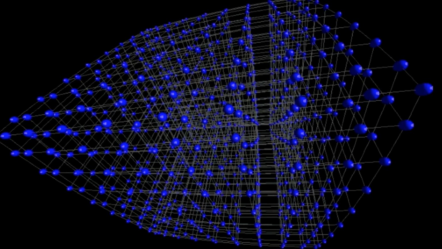
(a) ev1049_cube

http://ubiety.uwaterloo.ca/ubigraph/ev/ev1049_coarsening.mov

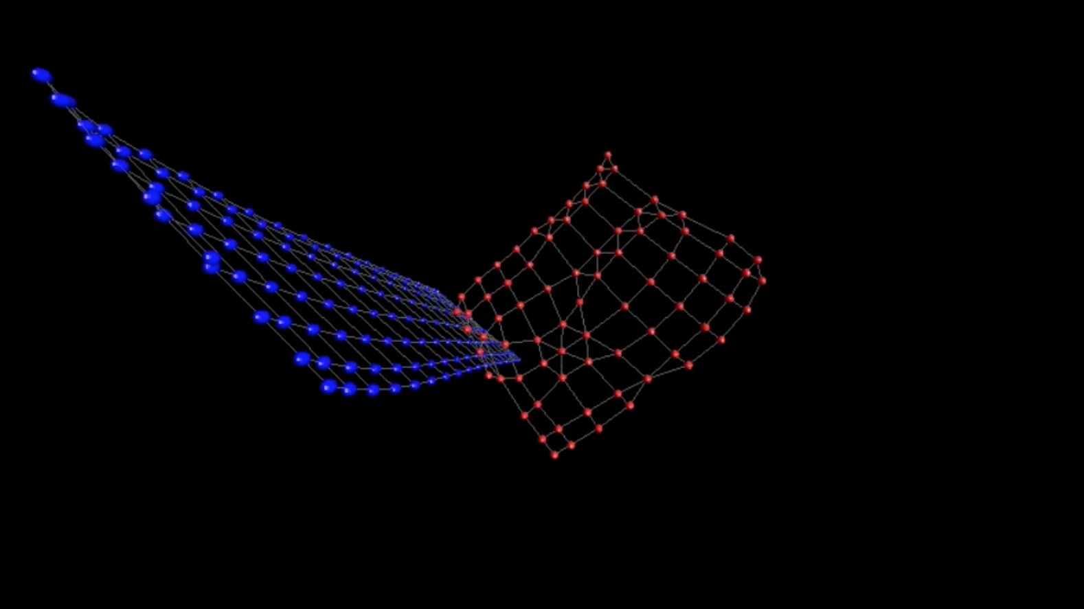
(b) ev1049_coarsening

http://ubiety.uwaterloo.ca/ubigraph/ev/ev1049_twolevel.mov

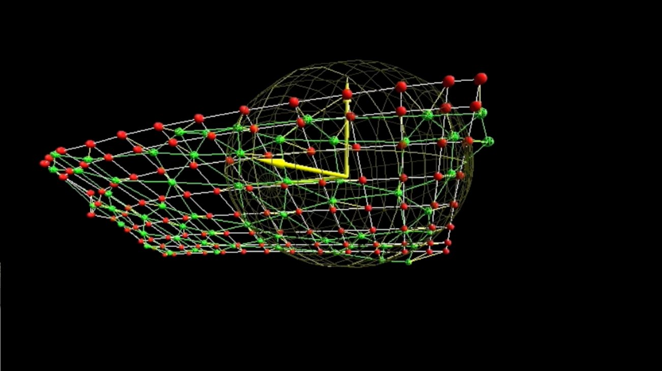
(c) ev1049_twolevel

http://ubiety.uwaterloo.ca/ubigraph/ev/ev1049_threelevel.mov

(d) ev1049_threelevel

http://ubiety.uwaterloo.ca/ubigraph/ev/ev1049_compare.mov

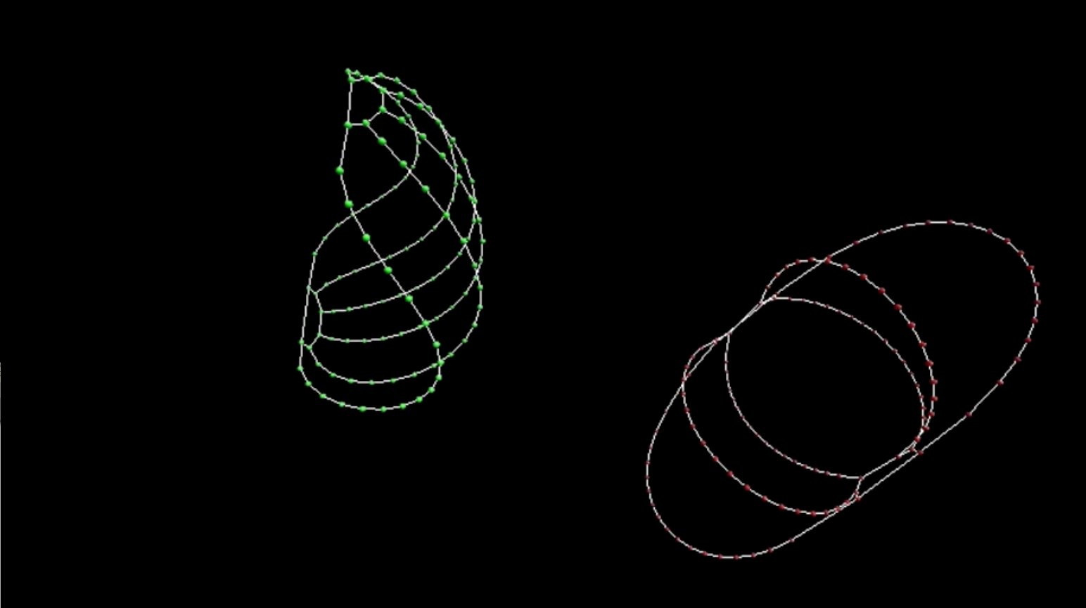
(e) ev1049_compare

http://ubiety.uwaterloo.ca/ubigraph/ev/ev1049_multilevel.mov

(f) ev1049_multilevel

http://ubiety.uwaterloo.ca/ubigraph/ev/ev1049_randomgraph.mov

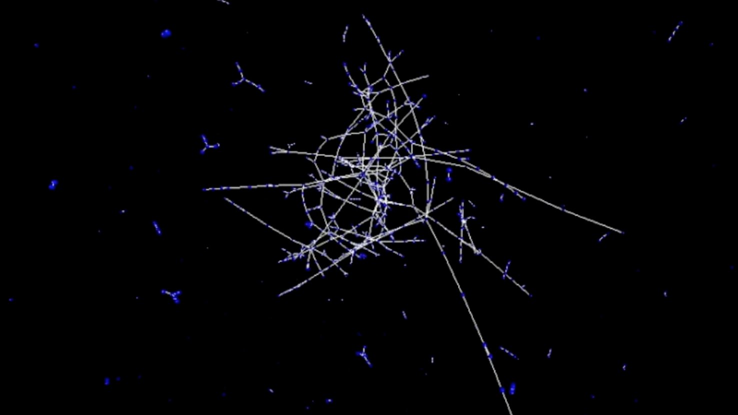
(g) ev1049_randomgraph

http://ubiety.uwaterloo.ca/ubigraph/ev/ev1049_tree.mov

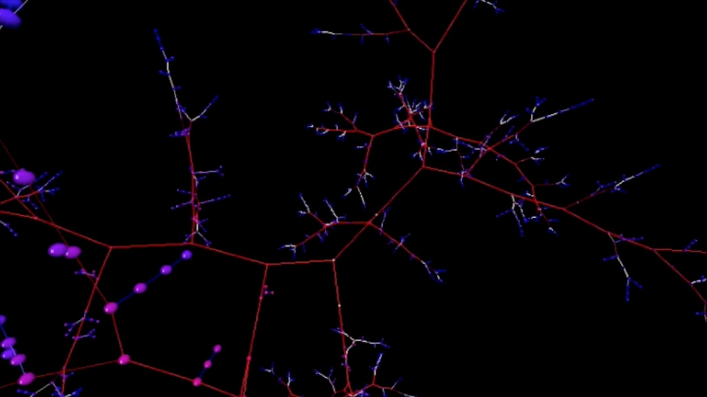
(h) ev1049_tree

Figure 1: Still frames from the demonstration movies accompanying this paper.

• http://ubiety.uwaterloo.ca/ubigraph/ev/ev1049_cube.movev1049_cube.mov: Layout of a 10x10x10 cube graph using single-level dynamics (Section 3.1), 8 cores, and Euler time steps.

• http://ubiety.uwaterloo.ca/ubigraph/ev/ev1049_coarsening.movev1049_coarsening.mov: Demonstration of the dynamic coarsening algorithm (Section 4).

• http://ubiety.uwaterloo.ca/ubigraph/ev/ev1049_twolevel.movev1049_twolevel.mov: Two-level dynamics, showing the projection dynamics and dynamic coarsening.

• http://ubiety.uwaterloo.ca/ubigraph/ev/ev1049_threelevel.movev1049_threelevel.mov: Three-level dynamics showing a graph moving quickly through assorted configurations. The coarsest graph is maintained automatically from modifications the first-level coarsener makes to the second graph.

• http://ubiety.uwaterloo.ca/ubigraph/ev/ev1049_compare.movev1049_compare.mov: Side-by-side comparison of single-level vs. three-level dynamics, illustrating the quicker convergence achieved by multilevel dynamics.

• http://ubiety.uwaterloo.ca/ubigraph/ev/ev1049_multilevel.movev1049_multilevel.mov: Showing quick convergence times using multilevel dynamics (4-6 levels) on static graphs being reset to random vertex positions.

• http://ubiety.uwaterloo.ca/ubigraph/ev/ev1049_randomgraph.movev1049_randomgraph.mov: Visualization of the emergence of the giant component in a random graph (Section 6). (8 cores, Euler step).

• http://ubiety.uwaterloo.ca/ubigraph/ev/ev1049_tree.movev1049_tree.mov: Visualization of rapid insertions into a binary tree (8 cores, Euler step).

2 Related work

Graph animation is widely used for exploring and navigating large graphs (e.g., [HMM00].) There is a vast amount of work in this area, so we focus on systems that aim to animate changing graphs.

Offline graph animation tools develop an animation from a sequence of key frames (layouts of static graphs). Such systems find layouts for key frame graphs, and then interpolate between the key frames in an appropriate way (e.g. [FE02]).

In contrast, our system tackles the problem of online or incremental graph layout. We use the term online in the sense of online algorithms: one receives a sequence of requests (in our case, changes to a graph), and each request must be processed without foreknowledge of future requests.

The key frame approach can be adapted to address the online problem by computing a new key frame each time a request arrives, and then interpolating to the new key frame. For example, Huang et al [HEW98] developed a system for browsing large, partially known graphs, where navigation actions add and remove subgraphs. They use force-directed layout for key frame graphs, and interpolate between them.

Another approach is to take an existing graph layout algorithm and incrementalize (or dynamize) it. For example, the Dynagraph system [NW01, EGK^∗04] uses an incrementalized version of the batch Sugiyama-Tagawa-Toda algorithm [STT81].

Our basic approach is to develop an incrementalized version of Walshaw’s multilevel force-directed layout algorithm [Wal03]. We perform a continuously running force-directed layout. When a graph change request arrives, the graph is immediately updated. This changes the potential function, so that the current layout is no longer an equilibrium position. The layout immediately starts to seek a new equilibrium. If the changes come rapidly enough, the graph will be in continuous motion. One advantage of this approach is that changes to the graph are shown immediately, without delaying to compute a key frame.

3 Layout Dynamics

We use Lagrangian dynamics to derive the equations of motion for the simulation. Lagrangian dynamics is a bit excessive for a simple springs-and-repulsion graph layout. However, we have found that convergence times are greatly improved by dynamically adapting the interpolation between coarser and finer graphs. For this we use generalized forces, which are easily managed with a Lagrangian approach.

As is conventional, we write $\dot{\boldsymbol{x}}_{i}$ for the velocity of vertex $i$, and $\ddot{\boldsymbol{x}}_{i}$ for its acceleration. We take all masses to be 1, so that velocity and momentum are interchangeable.

In addition to the potential energy $V$ (Eqn (1)), we define a kinetic energy $T$. For a single graph, this is simply:

$$T =\sum_{v_{i}\in V}\tfrac{1}{2}\|\dot{\boldsymbol{x}}_{i}\|^{2}$$ (2)

Roughly speaking, $T$ describes channels through which potential energy (layout badness) can be converted to kinetic energy (vertex motion). Kinetic energy is then dissipated through friction, which results in the system settling into a local minimum of the potential $V$. We incorporate friction by adding extra terms to the basic equations of motion.

The equations of motion are obtained from the Euler-Lagrange equation:

$$\left[\frac{d}{dt}\frac{\partial}{\partial\dot{\boldsymbol{x}}_{i}}-\frac{\partial}{\partial\boldsymbol{x}_{i}}\right]L =0$$ (3)

where the quantity $L=T-V$ is the Lagrangian.

3.1 Single level dynamics

The coarsest graph has straightforward dynamics. Substituting the definitions of (1,2) into the Euler-Lagrange equation yields the basic equation of motion $\ddot{\boldsymbol{x}}_{i}=\boldsymbol{F}_{i}$ for a vertex, where $\boldsymbol{F}_{i}$ is the net force:

$$\ddot{\boldsymbol{x}}_{i} =\underbrace{\sum_{v_{i},v_{j}}-K(\boldsymbol{x}_{i}-\boldsymbol{x}_{j})}_{\text{spring forces}}+\underbrace{\sum_{v_{j}\neq v_{i}}\frac{f_{0}}{(\epsilon_{R}+\|\boldsymbol{x}_{i}-\boldsymbol{x}_{j}\|)^{2}}\cdot\frac{\boldsymbol{x}_{i}-\boldsymbol{x}_{j}}{\|\boldsymbol{x}_{i}-\boldsymbol{x}_{j}\|}}_{\text{repulsion forces}}$$ (4)

We calculate the pairwise repulsion forces in $O(n\log n)$ time (with $n=|V|$, the number of vertices) using the Barnes-Hut algorithm [BH86].

The spring and repulsion forces are supplemented by a damping force defined by $\boldsymbol{F}^{d}_{i}=-d\dot{\boldsymbol{x}}_{i}$ where $d$ is a constant.

Our system optionally adds a ‘gravity’ force that encourages directed edges to point in a specified direction (e.g., down).

3.2 Two-level dynamics

We now describe how the dynamics of a graph interacts with its coarser version. For notational clarity we write $\boldsymbol{y}_{i}$ for the position of the coarse vertex corresponding to vertex $i$, understanding that each vertex in the coarse graph may correspond to multiple vertices in the finer graph.

In Walshaw’s static multilevel layout algorithm [Wal03], each vertex $\boldsymbol{x}_{i}$ simply uses as its starting position $\boldsymbol{y}_{i}$, the position of its coarser version. To adapt this idea to a dynamic setting, we begin by defining the position of $\boldsymbol{x}_{i}$ to be $\boldsymbol{y}_{i}$ plus some displacement $\boldsymbol{\delta}_{i}$, i.e.,:

$$\boldsymbol{x}_{i} =\delta_{i}+\boldsymbol{y}_{i}$$

However, in practice this does not work as well as one might hope, and convergence is faster if one performs some scaling from the coarse to fine graph, for example

$$\boldsymbol{x}_{i} =\delta_{i}+a\boldsymbol{y}_{i}$$

A challenge in doing this is that the appropriate scaling depends on the characteristics of the particular graph. Suppose the coarse graph roughly halves the number of vertices in the fine graph. If the fine graph is, for example, a three-dimensional cube arrangement of vertices with 6-neighbours, then the expansion ratio needed will be $\approx 2^{1/3}$ or about $1.26$; a two-dimensional square arrangement of vertices needs an expansion ratio of $\approx\sqrt{2}$ or about $1.41$. Since the graph is dynamic, the best expansion ratio can also change over time. Moreover, the optimal amount of scaling might be different for each axis, and there might be differences in how the fine and coarse graph are oriented in space.

Such considerations led us to consider affine transformations from the coarse to fine graph. We use projections of the form

$$\boldsymbol{x}_{i} =\boldsymbol{\delta}_{i}+\boldsymbol{\alpha}\boldsymbol{y}_{j}+\boldsymbol{\beta}$$ (5)

where $\boldsymbol{\alpha}$ is a linear transformation (a 3x3 matrix) and $\boldsymbol{\beta}$ is a translation. The variables $(\boldsymbol{\alpha},\boldsymbol{\beta})$ are themselves given dynamics, so that the projection converges to a least-squares fit of the coarse graph to the fine graph.

3.2.1 Frame dynamics

We summarize here the derivation of the time evolution equations for the affine transformation $(\boldsymbol{\alpha},\boldsymbol{\beta})$. Conceptually, we think of the displacements $\delta_{i}$ as “pulling” on the transformation: if all the displacements are to the right, the transformation will evolve to shift the coarse graph to the right; if they are all outward, the transformation will expand the projection of the coarse graph, and so forth. In this way the finer graph ‘pulls’ the projection of the coarse graph around it as tightly as possible.

We derive the equations for $\ddot{\boldsymbol{\alpha}}$ and $\ddot{\boldsymbol{\beta}}$ using Lagrangian dynamics. To simplify the derivation we pretend that both graph layouts are stationary, and that the displacements $\delta_{i}$ behave like springs between the fine graph and the projected coarse graph, acting on $\boldsymbol{\alpha}$ and $\boldsymbol{\beta}$ via ‘generalized forces.’ By setting up appropriate potential and kinetic energy terms, the Euler-Lagrange equations yield:

$$\ddot{\boldsymbol{\alpha}} =\tfrac{1}{n}\sum_{i}\boldsymbol{\delta}_{i}\boldsymbol{y}_{i}^{T}+\boldsymbol{y}_{i}\boldsymbol{\delta}_{i}^{T}$$ (6)

$$\ddot{\boldsymbol{\beta}} =\tfrac{1}{n}\sum_{i}\boldsymbol{\delta}_{i}$$ (7)

To damp oscillations and dissipate energy we introduce damping terms of $-d_{\alpha}\dot{\boldsymbol{\alpha}}$ and $-d_{\beta}\dot{\boldsymbol{\beta}}$.

3.2.2 Time dilation

We now turn to the equations of motion for vertices in the two-level dynamics. The equations for $\dot{\boldsymbol{\delta}}_{i}$ and $\ddot{\boldsymbol{\delta}}_{i}$ are obtained by differentiating Eqn (5):

$$\boldsymbol{x}_{i} =\boldsymbol{\delta}_{i}+\underbrace{\boldsymbol{\beta}+\boldsymbol{\alpha}\boldsymbol{y}_{i}}_{\text{proj. position}}$$ (8)

$$\dot{\boldsymbol{x}}_{i} =\dot{\boldsymbol{\delta}}_{i}+\underbrace{\dot{\boldsymbol{\beta}}+\dot{\boldsymbol{\alpha}}\boldsymbol{y}_{i}+\boldsymbol{\alpha}\dot{\boldsymbol{y}}_{i}}_{\text{proj. velocity}}$$ (9)

$$\ddot{\boldsymbol{x}}_{i} =\ddot{\boldsymbol{\delta}}_{i}+\underbrace{\ddot{\boldsymbol{\beta}}+\ddot{\boldsymbol{\alpha}}\boldsymbol{y}_{i}+2\dot{\boldsymbol{\alpha}}\dot{\boldsymbol{y}}_{i}+\boldsymbol{\alpha}\ddot{\boldsymbol{y}}_{i}}_{\text{proj. acceleration}}$$ (10)

Let $\boldsymbol{F}_{i}$ be the forces acting on the vertex $\boldsymbol{x}_{i}$. Substituting Eqn (10) into $\ddot{\boldsymbol{x}}_{i}=\boldsymbol{F}_{i}$ and rearranging, one obtains an equation of motion for the displacement:

$$\ddot{\boldsymbol{\delta}}_{i} =\boldsymbol{F}_{i}-\left(\underbrace{\ddot{\boldsymbol{\beta}}+\ddot{\boldsymbol{\alpha}}\boldsymbol{y}_{i}+2\dot{\boldsymbol{\alpha}}\dot{\boldsymbol{y}}_{i}+\boldsymbol{\alpha}\ddot{\boldsymbol{y}}_{i}}_{\text{proj. acceleration}}\right)$$ (11)

The projected acceleration of the coarse vertex can be interpreted as a ‘pseudoforce’ causing the vertex to react against motions of its coarser version. If Eqn (11) were used as the equation of motion, the coarse and fine graph would evolve independently, with no interaction. (We have used this useful property to check correctness of some aspects of our system.)

The challenge, then, is how to adjust Eqn (11) in some meaningful way to couple the finer and coarse graph dynamics. Our solution is based on the idea that the coarser graph layout evolves similarly to the finer graph, but on a different time scale: the coarse graph generally converges much more quickly. To achieve a good fit between the coarse and fine graph we might slow down the evolution of the coarse graph. Conceptually, we try to do the opposite, speeding up evolution of the fine graph to achieve a better fit. Rewriting Eqn (8) to make each variable an explicit function of time, and incorporating a time dilation, we obtain

$$\boldsymbol{x}_{i}(t) =\boldsymbol{\delta}_{i}(t)+\underbrace{\boldsymbol{\beta}(t)+\boldsymbol{\alpha}(t)\boldsymbol{y}_{i}(\phi t)}_{\text{proj. position}}$$ (12)

where $\phi$ is a time dilation factor to account for the differing time scales of the coarse and fine graph. Carrying this through to the acceleration equation yields the equation of motion

$$\ddot{\boldsymbol{\delta}}_{i} =\boldsymbol{F}_{i}-\left(\underbrace{\ddot{\boldsymbol{\beta}}+\ddot{\boldsymbol{\alpha}}\boldsymbol{y}_{i}+2\dot{\boldsymbol{\alpha}}\phi\dot{\boldsymbol{y}}_{i}+\boldsymbol{\alpha}\phi^{2}\ddot{\boldsymbol{y}}_{i}}_{\text{proj. acceleration}}\right)$$ (13)

If for example the coarser graph layout converged at a rate twice that of the finer graph, we might take $\phi=\tfrac{1}{2}$, with the effect that we would discount the projected acceleration $\ddot{\boldsymbol{y}}_{i}$ by a factor of $\phi^{2}=\tfrac{1}{4}$. In practice we have used values of $0.1\leq\phi\leq 0.25$. Applied across multiple levels of coarse graphs, we call this approach multilevel time dilation.

In addition to the spring and repulsion forces in $\boldsymbol{F}_{i}$, we include a drag term $\boldsymbol{F}_{i}^{d}=-d\dot{\boldsymbol{\delta}}_{i}$ in the forces of Eqn (13).

3.3 Multilevel dynamics

To handle multiple levels of coarse graphs, we iterate the two-level dynamics. The dynamics simulation simultaneously integrates the following equations:

• The equations of motion for the vertices in the coarsest graph, using the single-level dynamics of Section 3.1.

• The equations for the projection $\boldsymbol{\alpha},\boldsymbol{\beta}$ between each coarser and finer graph pair (Section 3.2.1).

• The equations of motion $\ddot{\boldsymbol{\delta}}_{i}$ for the displacements of vertices in the finer graphs, using the two-level dynamics of Section 3.2.

In our implementation, the equations are integrated using an explicit, fourth-order Runge-Kutta method. (We also have a simple Euler-step method, which is fast, but not as reliably stable.)

3.4 Equilibrium positions of the multilevel dynamics

We prove here that a layout found using the multilevel dynamics is an equilibrium position of the potential energy function of Eqn (1). This establishes that the multilevel approach does not introduce spurious minima, and can be expected to converge to the same layouts as a single-level layout, only faster.

Theorem 3.1.

Let $(X,\dot{X})$ be an equilibrium position of the two-level dynamics, where $X=(\boldsymbol{\delta}_{1},\boldsymbol{\delta}_{2},\ldots,\boldsymbol{\alpha},\boldsymbol{\beta},\boldsymbol{y}_{1},\boldsymbol{y}_{2},\ldots)$, and $\ddot{X}=\dot{X}=0$. Then, $(\boldsymbol{x}_{1},\boldsymbol{x}_{2},\ldots,\boldsymbol{x}_{n})$ is an equilibrium position of the single-level dynamics, where $\boldsymbol{x}_{i}=\boldsymbol{\delta}_{i}+\boldsymbol{\alpha}\boldsymbol{y}_{i}+\boldsymbol{\beta}$, and the single-level potential gradient $\nabla V=0$ (Eqn (1)) vanishes there.

Proof.

Since $\dot{X}=0$, the drag terms vanish from all equations of motion. Substituting $\dot{X}=0$ and $\ddot{X}=0$ into Eqn (13) yields $\boldsymbol{F}_{i}=0$ for each vertex. Now consider the single-level dynamics (Section 3.1) using the positions $\boldsymbol{x}_{i}$ obtained from $\boldsymbol{x}_{i}=\delta_{i}+\boldsymbol{\alpha}y_{i}+\boldsymbol{\beta}$ (Eqn (5)). From $\ddot{\boldsymbol{x}}_{i}=\boldsymbol{F}_{i}$ we have have $\ddot{\boldsymbol{x}}_{i}=0$ for each $i$. The Euler-Lagrange equations for the single level layout are (Eqn (3)):

$$\frac{d}{dt}\frac{\partial L}{\partial\dot{\boldsymbol{x}_{i}}}-\frac{\partial}{\partial\boldsymbol{x}_{i}}L =0$$

Since $\frac{d}{dt}\frac{\partial L}{\partial\dot{\boldsymbol{x}_{i}}}=\ddot{\boldsymbol{x}_{i}}=0$, we have $-\frac{\partial}{\partial\boldsymbol{x}_{i}}L=0$. Using $L=T-V$ and that the kinetic energy $T$ does not depend on $\boldsymbol{x}_{i}$, we obtain

$$\frac{\partial}{\partial\boldsymbol{x}_{i}}V=0$$

for each $i$. Therefore $\nabla V=0$ at this point. ∎

This result can be applied inductively over pairs of finer-coarser graphs, so that Theorem 3.1 holds also for multilevel dynamics.

4 Dynamic coarsening

As vertices and edges are added to and removed from the base graph $G=(V,E)$, our system dynamically maintains the coarser graphs $G_{1},G_{2},\ldots,G_{m}$. Each vertex in a coarse graph may correspond to several vertices in the base graph, which is to say, each coarse graph defines a partition of the vertices in the base graph. It is useful to describe coarse vertices as subsets of $V$. For convenience we define a finest graph $G_{0}$ isomorphic to $G$, with vertices $V_{0}=\{\{v\}~{}:~{}v\in V\}$, and edges $E_{0}=\{(\{v_{1}\},\{v_{2}\})~{}:~{}(v_{1},v_{2})\in E\}$. Coarser graphs are obtained by merging vertices via set union. The sequence $V_{0},V_{1},\ldots,V_{m}$ of of coarse graph vertices forms a chain in the lattice of partitions of $V$; we need to maintain this chain of partitions as changes are made to the base graph $V_{0}$.

We have devised an algorithm that efficiently maintains $G_{i+1}$ in response to changes in $G_{i}$. By applying this algorithm at each level the entire chain $G_{1},G_{2},\ldots,G_{m}$ is maintained.

We present a fully dynamic, Las Vegas-style randomized graph algorithm for maintaining a coarsened version of a graph. For graphs of bounded degree, this algorithm requires $O(1)$ operations on average per edge insertion or removal.

Our algorithm is based on the traditional matching approach to coarsening developed by Hendrickson and Leland [HL95]. Recall that a matching of a graph $G=(V,E)$ is a subset of edges $M\subseteq E$ satisfying the restriction that no two edges of $M$ share a common vertex. A matching is maximal if it is not properly contained in another matching. A maximal matching can be found by considering edges one at a time and adding them if they do not conflict with an edge already in $M$. (The problem of finding a maximal matching should not be confused with that of finding a maximum cardinality matching, a more difficult problem.)

4.1 Dynamically maintaining the matching

We begin by making the matching unique. We do this by fixing a total order $<$ on the edges, chosen uniformly at random. (In practice, we compute $<$ using a bijective hash function.) To produce a matching we can consider each edge in ascending order by $<$, adding it to the matching if it does not conflict with a previously matched edge. If $e_{1}<e_{2}$, we say that $e_{1}$ has priority over $e_{2}$ for matching.

Our basic analysis tool is the edge graph $G^{\ast}=(E,S)$ whose vertices are the edges of $G$, and $e_{1}Se_{2}$ when the edges share a vertex. A set of edges $M$ is a matching on $G$ if and only if $M$is an independent set of vertices in $G^{\ast}$. From $G^{\ast}$ we can define an edge dependence graph $\mathcal{E}=(E,\rightarrow)$ which is a directed version of $G^{\ast}$:

$$e_{1}\rightarrow e_{2} \equiv(e_{1}<e_{2})~{}\text{and}~{}e_{1}Se_{2}~{}\text{(share a common vertex)}$$

Since $<$ is a total order, the edge dependence graph $\mathcal{E}$ is acyclic. Figure 2 shows an example.

Figure 2: Illustration of dynamic coarsening. Top left: A graph with double lines indicating matched edges; Top right: its coarsened version, obtained by contracting matched edges; Middle: the edge dependence graph for the initial graph, using the (arbitrarily chosen) order $e_{6}<e_{2}<e_{3}<e_{7}<e_{5}<e_{1}<e_{4}$. Initially the matching is $\{e_{2},e_{6}\}$. Removing edge $e_{2}$ (bottom left) triggers re-evaluation of the match equations for $e_{5}$, $e_{1}$, and $e_{4}$. The new matching is $\{e_{6},e_{5},e_{1}\}$, resulting in changes to the coarsened graph (bottom right).

Building a matching by considering the edges in order of $<$ is equivalent to a simple rule: $e$ is matched if and only if there is no edge $e^{\prime}\in M$ such that $e^{\prime}\rightarrow e$. We can express this rule as a set of match equations whose solution can be maintained by simple change propagation. Let $m:E\rightarrow\{\bot,\top\}$ indicate whether an edge is matched: $m(e)=\top$ if and only if $e\in M$. The match equation for an edge $e\in E$ is:

$$m(e) =\bigwedge_{e^{\prime}~{}:~{}e^{\prime}\rightarrow e}\neg m(e^{\prime})$$

where by convention $\bigwedge\emptyset=\top$.

To evaluate the match equations we place the edges to be considered for matching in a priority queue ordered by $<$, so that highest priority edges are considered first. The match equations can then be evaluated using a straightforward change propagation algorithm:

While the priority queue is not empty:

1. Retrieve the highest priority edge $e=(v_{1},v_{2})$ from the queue and evaluate its match equation $m(e)$.

2. If the solution of the match equation has changed, then:

   1. If $m(e)=\top$, then $\mathrm{match}(v_{1},v_{2})$.

   2. If $m(e)=\bot$, then $\mathrm{unmatch}(v_{1},v_{2})$.

Both $\mathrm{match}(e)$ and $\mathrm{unmatch}(e)$ add the dependent edges of $e$ to the queue, so that changes ripple through the graph.

Figure 3 summarizes the basic steps required to maintain the coarser graph ($V^{\prime},E^{\prime}$) as edges and vertices are added and removed to the finer graph.

 

Dynamic-Match operations

We use $\overline{v}$ to indicate the coarse version of a vertex $v$.

• addEdge(e): Increase the count of $(\overline{v_{1}},\overline{v_{2}})$ in $E^{\prime}$ (possibly adding edge if not already present). Add $e$ to the queue.

• deleteEdge(e): If $e$ is in the matching then $\mathrm{unmatch}(e)$. Decrease the count of $(\overline{v_{1}},\overline{v_{2}})$ in $E^{\prime}$; if this count is 0 then delete this edge from $E^{\prime}$. If either $v_{1}$ or $v_{2}$ have no edges except $e$, then remove $\overline{v_{1}}$ (resp. $\overline{v_{2}}$) from the coarse graph. Add all edges $e^{\prime}$ with $e\rightarrow e^{\prime}$ to the queue.

• deleteVertex(v): for each edge $e$ incident on $v$, $\mathrm{deleteEdge}(e)$. Remove $v$ from $G$.

• addVertex(v): no action needed.

• $\mathrm{match}(e)$, where $e=(v_{1},v_{2})$: For each edge $e^{\prime}$ where $e\rightarrow e^{\prime}$, if $e^{\prime}$ is matched then $\mathrm{unmatch}(e^{\prime})$. Delete vertices $\overline{v_{1}}$ and $\overline{v_{2}}$ from the coarser graph. Create a new vertex $v_{1}\cup v_{2}$ in $G^{\prime}$. For all edges $e=(v,v^{\prime})$ in G incident on $v_{1}$ or $v_{2}$ (but not both), add a corresponding edge to or from $v_{1}\cup v_{2}$ in $G^{\prime}$. For each $e^{\prime}$ such that $e\rightarrow e^{\prime}$, add $e^{\prime}$ to the queue.

• $\mathrm{unmatch}(e)$, where $e=(v_{1},v_{2})$: delete any edges in $G^{\prime}$ incident on $v_{1}\cup v_{2}$. Delete the vertex $v_{1}\cup v_{2}$ from $G^{\prime}$. Add new vertices $\overline{v_{1}}$ and $\overline{v_{2}}$ to $G^{\prime}$. For each edge incident on $v_{1}$ or $v_{2}$ in $G$, add a corresponding edge to $G^{\prime}$. For each $e^{\prime}$ such that $e\rightarrow e^{\prime}$, add $e^{\prime}$ to the queue.

   

Figure 3: Basic operations of the dynamic coarsening algorithm.

4.2 Complexity of the dynamic matching

The following theorem establishes that for graphs of bounded degree, the expected cost of dynamically maintaining the coarsened graph is $O(1)$ per edge inserted or removed in the fine graph. The cost does not depend on the number of edges in the graph.

Theorem 4.1.

In a graph of maximum degree $d$, the randomized complexity of $\mathrm{addEdge}(e)$ and $\mathrm{removeEdge}(e)$ is $O(de^{2d})$.

We first prove a lemma concerning the extent to which updates may need to propagate in the edge dependence graph. As usual for randomized algorithms, we analyze the complexity using “worst-case average time,” i.e., the maximum (with respect to choices of edge to add or remove) of the expected time (with expectation taken over random priority assignments). For reasons that will become clear we define the priority order $<$ by assigning to each edge a random real in $[0,1]$, with $1$ being the highest priority.

Lemma 4.2.

Let $G^{\ast}=(E,S)$ be a graph and $\rho:E\rightarrow[0,1]$ an injective function chosen uniformly at random assigning to each vertex a real priority in $[0,1]$. If $G^{\ast}$ has maximum degree $k$, the expected number of vertices reachable from any vertex in $E$ following only edges from higher to lower priority vertices is $O(e^{k})$.

Figure 4: A linear arrangement of the edge dependence graph of Figure 2.

Proof.

It is helpful to view the priority assignment $\rho$ as inducing a linear arrangement of the vertices, i.e., we might draw $G^{\ast}$ by placing its vertices on the real line at their priorities. We obtain a directed graph $(E,\rightarrow)$ by making edges always point toward zero, i.e., from higher to lower priorities (cf. Figure 4). Note that vertices with low priorities will tend to have high indegree and low outdegree.

We write $\mathbb{E}[\cdot]$ for expectation with respect to the random priorities $\rho$. For $e\in E$, let $N(e)$ be the number of vertices of $G^{\ast}$ reachable from $e$ by following paths that move from higher to lower priority vertices. We bound the expected value of $N(e)$ given its priority $\rho(e)=\eta$: we can always reach $e$ from itself, and we can follow any edges to lower priorities:

$$\mathbb{E}[N(e)~{}|~{}\rho(e)=\eta] \leq 1+\sum_{e^{\prime}~{}:~{}eSe^{\prime}}\underbrace{\mathrm{Pr}(\rho(e^{\prime})<\eta)}_{=\eta}\cdot\mathbb{E}[N(e^{\prime})~{}|~{}\rho(e^{\prime})<\eta]$$ (14)

Let $f(\eta)=\sup_{e\in E}\mathbb{E}[N(e)~{}|~{}\rho(e)=\eta]$. Then,

$$\mathbb{E}[N(e^{\prime})~{}|~{}\rho(e^{\prime})<\eta] \leq\int_{0}^{\eta}\eta^{-1}f(\alpha)d\alpha$$ (15)

where the integration averages $f$ over a uniform distribution on priorities $[0,\eta)$. Since the degree of any vertex is $\leq k$, there can be at most $k$ terms in the summation of Eqn (14). Combining the above, we obtain

$$f(\eta) =\sup_{e\in E}\mathbb{E}[N(e)~{}|~{}\rho(e)=\eta]$$ (16)

$$\leq\sup_{e\in E}\left(1+\sum_{e^{\prime}Se}\eta\mathbb{E}[N(e^{\prime})~{}|~{}\rho(e^{\prime})<\eta]\right)$$ (17)

$$\leq 1+k\eta\int_{0}^{\eta}\eta^{-1}f(\alpha)d\alpha$$ (18)

$$\leq 1+k\int_{0}^{\eta}f(\alpha)d\alpha$$ (19)

Therefore $f(\eta)\leq g(\eta)$, where $g$ is the solution to the integral equation

$$g(\eta) =1+k\int_{0}^{\eta}g(\alpha)d\alpha$$ (20)

Isolating the integral and differentiating yields the ODE $g(\eta)=k^{-1}g^{\prime}(\eta)$, which has the solution $g(\eta)=e^{\eta k}$, using the boundary condition $g(0)=1$ obtained from Eqn (20). Since $0\leq\eta\leq 1$, $g(\eta)\leq e^{k}$. Therefore, for every $e\in E$, the number of reachable vertices satisfies $\mathbb{E}[N(e)]\leq e^{k}$. ∎

Note that the upper bound of $O(e^{k})$ vertices reachable depends only on the maximum degree, and not on the size of the graph.

We now prove Theorem 4.1.

Proof.

If a graph $G=(V,E)$ has maximum degree $d$, its edge graph $G^{\ast}$ has maximum degree $2(d-1)$. Inserting or removing an edge will cause us to reconsider the matching of $\leq e^{2(d-1)}$ edges on averages by Lemma 4.2. If a max heap is used to implement the priority queue, $O(de^{2d})$ operations are needed to insert and remove these edges. Therefore the randomized complexity is $O(de^{2d})$. ∎

In future work we hope to extend our analysis to show that the entire sequence of coarse graphs $G_{1},G_{2},\ldots,G_{m}$ can be efficiently maintained. In practice, iterating the algorithm described here appears to work very well.

5 Implementation

Our system is implemented in C++, using OpenGL and pthreads. The graph animator runs in a separate thread from the user threads. The basic API is simple, with methods $\mathrm{newVertex}()$ and $\mathrm{newEdge}(v_{1},v_{2})$ handling vertex and edge creation, and destructors handling their removal.

For static graphs, we have so far successfully used up to six levels of coarsening, with the coarsened graphs computed in advance. With more than six levels we are encountering numerical stability problems that seem to be related to the projection dynamics.

For dynamic graphs we have used three levels (the base graph plus two coarser versions), with the third-level graph being maintained from the actions of the dynamic coarsener for the first-level graph. At four levels we encounter a subtle bug in our dynamic coarsening implementation we have not yet resolved.

5.1 Parallelization

Our single-level dynamics implementation is parallelized. Each frame entails two expensive operations: rendering and force calculations. We use the Barnes-Hut tree to divide the force calculations evenly among the worker threads; this results in good locality of reference, since vertices that interact through edge forces or near-field repulsions are often handled by the same thread. Rendering is performed in a separate thread, with time step $t$ being rendered while step $t+\delta t$ is being computed. The accompanying animations were rendered on an 8-core (2x4) iMac using OpenGL, compiled with g++ at -O3.

Our multilevel dynamics engine is not yet parallelized, so the accompanying demonstrations of this are rendered on a single core. Parallelizing the multilevel dynamics engine remains for future work.

6 Applications

We include with this paper two demonstrations of applications:

• The emergence of the giant component in a random graph: In Erdös-Renyi $G(n,p)$ random graphs on $n$ vertices where each edge is present independently with probability $p$, there are a number of interesting phase transitions: when $p<n^{-1}$ the largest connected component is almost surely of size $\Theta(\log n)$; when $p=n^{-1}$ it is a.s. of size $\Theta(n^{2/3})$, and when $p>n^{-1}$ it is a.s. of size $\Theta(n)$—the “giant component.” In this demonstration a large random graph is constructed by preassigning to all ${n\choose 2}$ edges a probability trigger in $[0,1]$, and then slowly raising a probability parameter $p(t)$ from $0$ to $1$ as the simulation progresses, with edges ‘turning on’ when their trigger is exceeded.

• Visualization of insertions of random elements into a binary tree, with an increasingly rapid rate of insertions.

In addition, we mention that the graph visualizer was of great use in debugging itself, particularly in tracking down errors in the dynamic matching implementation.

7 Conclusions

We have described a novel approach to real-time visualization of dynamic graphs. Our approach combines the benefits of multilevel force-directed graph layout with the ability to render rapidly changing graphs in real time. We have also contributed a novel and efficient method for dynamically maintaining coarser versions of a graph.

References

- [BH86] Barnes J. E., Hut P.: A hierarchical force-calculation algorithm. Nature 324, 6270 (1986), 446–449.
- [Ead84] Eades P.: A heuristic for graph drawing. Congressus Numerantium 42 (1984), 149–160.
- [EGK∗04] Ellson J., Gansner E. R., Koutsofios E., North S. C., Woodhull G.: Graphviz and dynagraph – static and dynamic graph drawing tools. In Graph Drawing Software, Jünger M., Mutzel P., (Eds.), Mathematics and Visualization. Springer, 2004, pp. 127–148.
- [FE02] Friedrich C., Eades P.: Graph drawing in motion. J. Graph Algorithms Appl 6, 3 (2002), 353–370.
- [FLM94] Frick A., Ludwig A., Mehldau H.: A fast adaptive layout algorithm for undirected graphs. In Graph Drawing (1994), Tamassia R., Tollis I. G., (Eds.), vol. 894 of Lecture Notes in Computer Science, Springer, pp. 388–403.
- [FR91] Fruchterman T. M. J., Reingold E. M.: Graph drawing by force-directed placement. Softw. Pract. Exper. 21, 11 (1991), 1129–1164.
- [HEW98] Huang M. L., Eades P., Wang J.: On-line animated visualization of huge graphs using a modified spring algorithm. J. Visual Languages and Computing 9, 6 (Dec. 1998), 623–645.
- [HL95] Hendrickson B., Leland R.: An improved spectral graph partitioning algorithm for mapping parallel computations. SIAM Journal on Scientific Computing 16, 2 (Mar. 1995), 452–469.
- [HMM00] Herman, Melançon G., Marshall M. S.: Graph visualization and navigation in information visualization: A survey. IEEE Transactions on Visualization and Computer Graphics 6, 1 (Jan./Mar. 2000), 24–43.
- [KCH02] Koren Y., Carmel L., Harel D.: ACE: A fast multiscale eigenvectors computation for drawing huge graphs. In INFOVIS ’02: Proceedings of the IEEE Symposium on Information Visualization (InfoVis’02) (Washington, DC, USA, 2002), IEEE Computer Society, p. 137.
- [KK89] Kamada T., Kawai S.: An algorithm for drawing general undirected graphs. Inf. Process. Lett. 31, 1 (1989), 7–15.
- [NW01] North S. C., Woodhull G.: Online hierarchical graph drawing. In Graph Drawing (2001), Mutzel P., Jünger M., Leipert S., (Eds.), vol. 2265 of Lecture Notes in Computer Science, Springer, pp. 232–246.
- [STT81] Sugiyama K., Tagawa S., Toda M.: Methods for visual understanding of hierarchical systems. IEEE Transactions on Systems, Man, and Cybernetics 11, 4 (1981), 109–125.
- [Wal03] Walshaw C.: A multilevel algorithm for force-directed graph drawing. J. Graph Algorithms Appl. 7, 3 (2003), 253–285.