11email: nicole.meyer@obspm.fr 22institutetext: SUBATECH, IN2P3/CNRS, Université de Nantes, Ecole des Mines de Nantes, and Observatoire de Paris; 4 rue Alfred Kastler, 44307 Nantes, France
Radio pulses from cosmic ray air showers
High-energy cosmic rays passing through the Earth’s atmosphere produce extensive showers whose charges emit radio frequency pulses. Despite the low density of the Earth’s atmosphere, this emission should be affected by the air refractive index because the bulk of the shower particles move roughly at the speed of radio waves, so that the retarded altitude of emission, the relativistic boost and the emission pattern are modified. We consider in this paper the contribution of the boosted Coulomb and the Čerenkov fields and calculate analytically the spectrum using a very simplified model in order to highlight the main properties. We find that typically the lower half of the shower charge energy distribution produces a boosted Coulomb field, of amplitude comparable to the levels measured and to those calculated previously for synchrotron emission. Higher energy particles produce instead a Čerenkov-like field, whose amplitude may be smaller because both the negative charge excess and the separation between charges of opposite signs are small at these energies.
Key Words.:
radiation mechanisms: non-thermal - waves - elementary particles - cosmic rays1 Introduction
Nearly a century after the discovery of cosmic rays, their nature and origin still constitute one of the great problem of contemporary astrophysics. Most of them are revealed by their electromagnetic radiation, but those reaching the solar system play a unique role since they can be observed nearly directly. The extensive air showers made of secondary (or higher order) particles produced by high-energy cosmic rays in the Earth’s atmosphere are currently studied with giant ground-based particle detectors, whereas additional information is provided by observing fluorescence and Čerenkov radiation in the optical range.
A complementary technique is being developed, based on the detection of radio emission from the shower charged particles, making advantage of the techniques of increasing sophistication developed for radioastronomy. Indeed, it has been known for several decades that the charges in extensive cosmic ray showers produce radio frequency pulses, as first suggested by Askar’yan (ask62 (1962)) who estimated the Čerenkov emission. Subsequent studies (see Kahn & Lerche kah66 (1966)) have suggested radio emission to be produced instead by acceleration by the Lorentz force in the Earth’s magnetic field (see the extensive review by Allan all71 (1971)), and have stimulated extensive calculations and modelling of the synchrotron radiation (see Huege & al. hue07 (2007) and refs. therein). Up to now, the difficulties in both theory and observation have precluded a full understanding of the origin of the radio emission.
Most previous studies of this radio emission have approximated the air refractive index by unity. However, the median energy of electrons in the shower is about 30 MeV, corresponding to ; the median speed is thus greater than the phase speed of radio waves in air at sea level (where ), and is roughly equal to the phase speed at an altitude of half the atmospheric scale height. The air refractive index may thus affect significantly the radio electric field produced by the shower, whatever the emission mechanism, by changing the retarded altitude, the relativistic boost and the radiation pattern.
In particular, this should increase the relativistic boost of the Coulomb field produced by the shower charges, at speeds slightly smaller than the wave phase speed, whereas faster charges, which can catch up with the waves they emit, produce a Čerenkov like field. We make below an analytical calculation of these fields with a highly simplified model of the charge distribution, in order to highlight the physical processes and evaluate the contributions to the total electric field.
Before taking the refractive index into account, let us estimate the boosted Coulomb field produced in vacuum by a shower particle. Consider a charge in uniform relativistic motion. For an observer at rest, the Coulomb field is radial relative to the instantaneous present position of the charge, but the FitzGerald-Lorentz contraction compresses the field lines, so that in the directions normal to the velocity, the field in vacuum is greater than the isotropic Coulomb field by the Lorentz factor . This produces a pulse of electric field of maximum amplitude when the charge’s path passes at closest distance to the antenna, and of temporal width , directed from the charge’s present position to the observation point. The number of charges in the shower at maximum development is about one per GeV of primary energy with about 20% relative excess of electrons over positrons. With a primary cosmic ray of eV, i.e. charges, and a median secondary energy of 30 MeV (), this yields a pulse of maximum amplitude a few V/m and of duration roughly 10 ns at 100 m perpendicular distance. The corresponding low-frequency Fourier transform is a few V/m/MHz at frequencies smaller than MHz. The exact strength and polarisation are determined by the magnetic charge separation which produces oppositely directed changes of position and velocity for charges of opposite signs. This field should be added to the contribution of synchrotron emission.
Since the above amplitude is of the same order of magnitude as the values observed by different instruments (see Allan all71 (1971), Ardouin ard06 (2006), Horneffer hor06 (2006)), this contribution may not be negligible. We therefore consider this field in more detail, taking the refractive index into account.
2 Electric field spectrum of a subluminal charge
In this Section, we consider a point charge. A charge distribution and the corresponding coherence effects will be considered in Section 4.
2.1 Retarded potentials
Consider a point charge moving in a medium of constant refractive index (and relative magnetic permeability ), at velocity . The field potentials at space-time point () are the standard Liénard-Wiechert potentials with the formal replacements and
| (1) | |||||
| (2) |
where , is the unit vector in the direction of the point of observation from the moving charge, is the distance to the moving charge, and the subscript “ret” on the square bracket indicates that the quantities inside are to be evaluated at the (observer’s) retarded time (see for example Feynman fey64 (1964), Jackson jac99 (1999), Thidé thi97 (1997)).
Equations (1)-(2) hold whatever the charge’s motion and the refractive index, provided is a constant. Namely, this formulation neglects both the variation of with position and the dispersion, in particular the variation of with frequency (Ginzburg gin89 (1989), Clemmow & Dougherty cle69 (1994)). In this paper we will apply these equations for a uniform velocity, so that the electric field, given by (15), is the acceleration-independent term of the Liénard-Wiechert electric field (see for example Feynman fey64 (1964), Jackson jac99 (1999)), i.e. mainly a boosted Coulomb field for a subluminal charge or a Čerenkov-like field for a supraluminal charge. This field should be added to the synchrotron field calculated by the current models of shower emission. In the present Section, we consider the first case: smaller than the velocity of light in the medium , i.e. .

In this case, only one instant in the charge’s past history has a light cone that reaches a given location in space-time (), so that there is only one retarded time for a given (). Let us take the origin of (observer’s) co-ordinates so that the charge moving along the axis passes at at , and let us put an electric antenna at co-ordinate along the charge’s path, and distance in the perpendicular plane along the axis (Fig.1). This choice of origin allows to keep the time of arrival of the charge in the results, which will be used in Sections 4 and 6 to evaluate coherence effects for a source of finite size.
The distance between the charge’s present and past positions is PP’, so that with the notations of Fig.1, P’Q, whence AQ. From the triangles CPA and QPA we have AQ, so that, since , the square of the denominator in the bracket of (1) is
| (3) |
Equation (3) is a purely geometrical relation which holds whatever the sign of , provided at least one point P’ (source’s retarded position) does exist. This is the case when the right-hand side term of (3) is positive or zero, a condition which always holds for the subluminal case (), and which defines the Čerenkov cone for . We shall consider the latter case in Section 5.
Substituting (3) into (1) yields
| (4) |
where
| (5) |
Note that we have used an absolute value in (5), although for a subluminal charge, in order to be able to use the same definition of for a supraluminal charge (Section 5).
Equations (4) and (2) yield a pulse in the potentials, centred at , the time when the charge’s trajectory passes at closest approach to the antenna, and of half-width about . In the limit , (4) reduces to the well-known potential of a point charge in uniform motion in vacuum (see for example Feynman fey64 (1964), Jackson jac99 (1999)).
It is important to recall that in (4), the relevant charge and velocity are retarded quantities. Namely, the potentials only depend on the charge, position and speed of the particle at the retarded time. This means that the pulse’s peak is produced by the past state of the charge, at the retarded time , when the charge was at distance from the antenna along the direction of motion. Since at the time of the peak of potential at the antenna (A), the charge’s position (P) is at C so that , we have at this time, whence
| (6) |
The state of the charge at times different from the retarded time that produce the pulse is irrelevant. In particular, the instant of the peak is that at which the charge moving at along the axis passes at closest approach to the antenna, but the real charge need not necessarily be there at this time; it may have disappeared or have changed its trajectory; the latter effects do not change the potentials, but produce an additional contribution to the electric field (15) due to the term (see Feynman & al. fey64 (1964)).
For cosmic showers, therefore, the relevant charge and speed producing the field are those corresponding to the development of the shower at the retarded altitude, given by (6); hence they do not necessarily correspond to maximum shower development. For an antenna on the ground and a shower inclined to the vertical by the angle , we see from Fig.1 and Eq.(6) that the retarded altitude is GP’, i.e.
| (7) |
where the signs and correspond respectively to the charge impacting the ground after or before the time of closest approach. For , , CP’ is much greater than GC, so that (7) yields approximately
| (8) |
where we have also omitted the factor . We shall return to the retarded altitude later.
From (4), we deduce immediately the component of the electric field
| (9) |
2.2 Effect of the refractive index
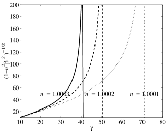
For relativistic velocities, the refractive index plays an important role, even though it is close to . Indeed, we see from (4)-(5) that a subluminal charge of Lorentz factor in a medium of refractive index produces the same electric potential as a charge of Lorentz factor
| (10) |
in vacuum. In particular, the pulse maximum amplitude and retarded altitude are both proportional to , whereas the time duration is inversely proportional to .
Figure 2 shows the factor as a function of for different values of the air refractive index. One sees that, as we noted in the introduction, the subluminal upper limit takes place at an energy of the same order of magnitude as the median energy of shower charges (). Note that for , , we have , so that may be approximated by
| (11) |
In practice, since the refractive index decreases as altitude increases, the retarded distance should be evaluated by an integration involving the wave phase speed at different altitudes from emission to reception. Since the greater the refractive index, the greater the propagation time, this integral is mainly determined by the greater values of the index. To simplify the calculations, we thus approximate the index by its value at low to mid altitudes, , but will keep in mind that is roughly proportional to the air density, decreasing roughly exponentially with altitude, and increasing with humidity (see for example Birch bir94 (1994)), which may have important consequences.
With this value of , we see from (11) that only for significantly smaller than , i.e. for electrons of energy significantly smaller than about 25 MeV. Since the median electron energy in a typical shower is about 30 MeV (), the radio electric field is expected to be rather different from its value in vacuum. For example, electrons of (respectively 40) in air with the above value of produce a similar electric field as electrons having (respectively 67) in vacuum.
Close to , i.e. , varies very rapidly. In this region, two physical effects come into play:
-
•
the variation of the refractive index, since is very sensitive to in this region,
-
•
the strong increase of the retarded altitude with , which tends to put it above the atmosphere, so that the retarded charge becomes negligible.
For example, at perpendicular distance m and vertical inclination angle , (8) yields 20 km for , i.e. . Hence in that case, for the retarded altitude not to be above the region of shower development, the energy of the radiating electrons should be smaller than about 24 MeV. This means that, since the median energy is about 30 MeV), typically a little less than the lower half of the electron energy distribution in the shower contribute to the boosted Coulomb electric field, for these values of perpendicular distance and angle to the vertical.
For greater energies, the retarded altitude is above the atmosphere, except for showers of large inclinations or passing very close to the antenna. And at energies so that , becomes imaginary; in that case, there is no longer a single retarded time and position, and a Čerenkov field is produced, which we shall evaluate in Section 5.
2.3 Electric field spectrum
Defining the Fourier transforms of the potentials as
| (12) |
| (13) | |||||
| (14) |
Here is a modified Bessel function of order 1 (Abramowitz & Stegun abr72 (1972)), is given by (5), is the antenna’s co-ordinate along the charge’s path (whose origin is the charge’s co-ordinate at ), and is the antenna’s perpendicular distance to the charge’s path.
The electric field is given by
| (15) |
so that its Fourier transform has from (13)-(14) the components
| (16) | |||||
| (17) |
Therefore for , , so that the electric field is radial (perpendicular to , directed along the charge’s present position to the antenna) of amplitude
| (18) |
with given by (10), at perpendicular distance from the charge’s path.
Using the expansions of the Bessel function (Abramowitz & Stegun abr72 (1972)), (18) yields at respectively low and high frequencies (or distances)
| (19) | |||||
| (20) |
for , . The low-frequency (or small distance) spectrum (the time integral of the pulse) is independent of , as expected since the larger , the greater the amplitude of the pulse, but the smaller (in the same proportion) the duration. At large frequencies and/or distances, the field decreases nearly exponentially with the product , thus with a frequency scale proportional to and a distance scale proportional to . At intermediate frequencies, the factor in (20) makes the decrease with (respectively ) slower (respectively faster) than given by the exponential alone.
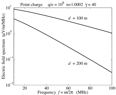
Figure 3 shows the modulus of the electric field spectrum (18) produced by a charge with ( being the electron charge) for and (), at perpendicular distances and 200 m, for which the retarded altitude (8) is respectively 5 and 10 km at a vertical angle .
Note that the plotted values correspond to Fourier transforms (defined as in (12)), so that they should be multiplied by a factor of two when comparing them to measured spectra, which are generally defined for positive frequencies only.
3 Charge at the retarded altitude
The retarded charge producing the pulse is that corresponding to the shower development at the retarded altitude, given by (8) as a function of the perpendicular distance to the path and of the inclination to the vertical. In the region of maximum shower development, the number of charged particles (mainly electrons and positrons) is
| (21) |
for a primary of energy , where eV (see for example Abu-Zayyad, & al. abu01 (2001) and references therein).
With a simplified atmosphere model of density at altitude , the total mass from the top of the atmosphere down to altitude is
| (22) |
where m and kg/m3. The altitude where the shower charge is maximum is determined by , where kg/m2 for a primary cosmic ray of energy eV, and increases at higher energies (Abu-Zayyad, & al. abu01 (2001) and references therein). The number of charged particles at the retarded altitude is determined by the value of . It can be obtained from the Greisen function as
| (23) |
where the so-called shower age is , is given by (21), and kg/m2 ( Abu-Zayyad, & al. abu01 (2001)).
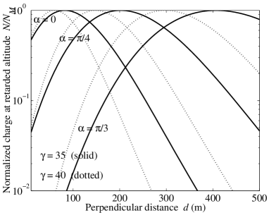
Figure 4 shows as a function of the perpendicular distance for different values of the inclination of the shower to the vertical, for and 40 with (respectively and 67).
At normal incidence, the number of charges at the retarded altitude is of the same order of magnitude as the value at maximum development, up to distances of a few hundred metres, for which the retarded altitude goes above the region of significant shower development. As the angle increases, the distance for which the retarded altitude is in the region of maximum development increases. The larger and , the larger the value of for which the retarded altitude corresponds to maximum shower development. As increases significantly above 45 (for ), the fast increase of puts the retarded altitude above the atmosphere.
In the following Section, we will thus consider charges of Lorentz factor .
4 Boosted Coulomb spectrum of a charge distribution

In the previous Sections, we have calculated the electric field of a point charge. However, the charge distribution in the shower is believed to be pancake shaped, of axis the shower direction, and of lateral size increasing with altitude. The half-size containing the bulk of the particles is about 20-30 m at ground level, somewhat smaller than the canonical Molière radius of about 80 m (Antoni & al. ant01 (2001)), and very thin in the longitudinal direction, with a dispersion in particle arrival times of about 1.6 ns at the centre (Linsley lin86 (1986)). This small longitudinal dispersion will decrease the field level because of the loss of coherence due to the factor in the spectrum (18).
With an axial symmetry, it is convenient to consider first a charge distributed round a circle of radius in the plane perpendicular to the path, infinitely thin in the direction, which allows an analytical calculation. The field of an arbitrary charge distribution can then be obtained by performing an integration over the lateral and longitudinal dimensions.
4.1 Ring charge distribution
Consider a charge distributed round a circle of radius in the plane perpendicular to which passes at at . The potential produced at perpendicular distance from the centre of the circle (and co-ordinate along the charge’s path) is, from (13) with the geometry defined in Fig.5
| (24) | |||||
| (25) | |||||
| (26) |
The integral can be calculated analytically by expanding in series of Bessel functions using Neumann’s addition theorem (Watson wat66 (1966)), from which we derive finally
| (27) | |||||
| (28) |
We deduce from (15) the (radial) electric field
| (29) | |||||
| (30) |
which has a discontinuity on the circle (as expected), of no physical consequence since it disappears on integration over the radius . Comparing to the electric field spectrum (18) of a point charge, we see that the finite size of the source removes the singularity of the field at . It also increases the field strength outside the source by the factor , which increases as frequency increases, so that the lateral size of the charge makes the spectrum at large distances fall less quickly with frequency than that of a point charge.
4.2 Pancake charge distribution
Consider now a charge of lateral distribution and finite longitudinal thickness. The potential at perpendicular distance from the centre is obtained by integrating (24) as
| (31) |
for a distribution normalised so that . Here involves an integral of the phase factor in Eq.(24), ponderated by the longitudinal source distribution. The longitudinal extension therefore decreases the spectrum at frequencies , where is the width of the particle arrival time distribution, because of loss of coherence, so that we have for , whereas for when the fields no longer add in phase.
We model the lateral distribution with the so-called NKG lateral density parametrization (see Nishimura nis67 (1967)). Here the two parameters and are not necessarily the conventional shower age and Molière radius respectively, since a wide set of couples can fit the observed lateral distribution (see Antoni & al. ant01 (2001) and refs. therein). However, the coupled variation of these parameters keeps roughly the same proportion of particles within a given lateral distance; for example, KASCADE measurements shown in Fig. 4 of the paper cited above find nearly 50% (respectively 80%) of the electrons within 20 m (respectively 50 m) lateral distance.
The distribution of arrival times is still less well known. Assuming ns at the centre of the pancake, and a value roughly three times greater at 30 m lateral distance (Linsley lin86 (1986)), the factor should decrease below unity at frequencies above about 50 MHz. In this highly simplified calculation, we will therefore neglect this effect and the curvature of the pancake, keeping in mind that the corresponding loss of coherence should decrease the spectrum above about 50 MHz.
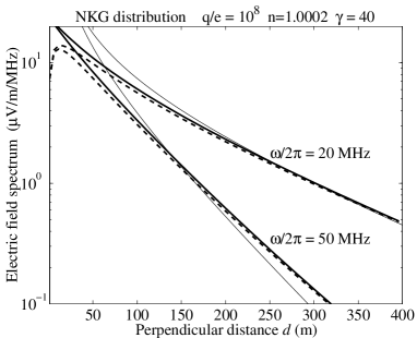
Figure 6 shows the boosted Coulomb electric field spectrum produced by electrons with a NKG distribution with two sets of parameters: [ m] and [ m], at frequencies and 50 MHz, as a function of the perpendicular distance to the charge’s path, for and , compared to the field of a point charge. One sees that the degeneracy of the parameters of the lateral distribution only affects the field at very short radial distances, where it is smaller than that of a point charge by a factor depending on the parameters of the distribution. At distances greater than about 50 m, the field does not depend significantly on the details of the charge distribution, in the frame of this highly simplified model.
4.3 Charge separation by the Lorentz force
If there were no systematic separation of positive and negative charges by the Earth’s magnetic field, the net charge producing the radio pulse would be equal to , where is given in (23) and is the relative excess of electrons over positrons in the shower, which amounts to about 20 % at low energies.
However, the Lorentz force due to the Earth’s magnetic field separates the positive and negative charges in the direction . The boosted Coulomb electric field is thus the geometric sum of those produced by the positive and negative charges, each being directed along the perpendicular distance to their respective charge’s barycentre, with opposite signs. The net electric field is then no longer directed along the perpendicular distance to the centre of the shower. For example, for a vertical shower impacting North of an antenna, this produces a Coulomb field having a East-West component, of strength roughly proportional to the separation between positive and negative charges.
Let us estimate the average displacement for electrons of Lorentz factor . The force acting during the time produces a displacement , in the plane perpendicular to , directed normal to the projection of in this plane. The time for travelling a radiation length divided by the air density is , and the average of is , so that the average displacement of electrons is
| (32) |
where is the angle between the magnetic field and the shower direction. With kg/m2, so that s at sea level, and G, this yields
| (33) |
With and , this yields m at sea level and m at an altitude of half the atmospheric scale height. Positrons are displaced in the opposite direction, producing a separation of . Allan (all71 (1971)) finds values somewhat greater, but of the same order of magnitude.
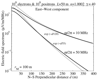
As an example, Fig. 7 shows the electric field spectrum projected on the East-West direction, as a function of distance to the centre along the NS axis, produced at and 50 MHz by electrons and positrons in vertical motion, displaced laterally by 50 m in opposite senses along the East-West direction, for and (); each charge species is assumed to have a NKG distribution with and m (solid lines). Exponential decreases are shown for comparison (dotted). Comparing to the case of point charges (thin lines), one sees that in this simple model, the field is not much affected by the NKG lateral distribution, except at very short distances.
As an example of the change in polarisation introduced by the magnetic field, Fig. 8 shows contours of the East-West and North-South components of the boosted Coulomb electric field spectrum produced at 20 MHz by electrons and positrons in vertical motion, displaced laterally by 50 m in opposite senses along the East-West direction; solid and dashed lines distinguish the sign of the field components; and have the same values as in Fig.7.
Note that the excess of electrons over positrons, not taken into account in this plot, produces an additional contribution changing both polarisation and amplitude.

5 Electric field spectrum of a supraluminal charge
Consider now a point charge moving faster than the waves, so that . This will produce a Čerenkov field instead of a boosted Coulomb field.
5.1 Retarded potentials
As we noted in Section 2, the retarded potentials are still given by Eqs.(1)-(3), but the geometry is different from Fig. 1 since now PP’ . This means that P is on the other side of C on the axis, at a distance so that . Therefore, the retarded source’s distance is now given by
| (34) |
which has two solutions if
| (35) |
i.e. with given by (5). When this inequality holds, the antenna is inside the Čerenkov cone of half-angle trailing the charge. When the opposite inequality holds, there is no solution for the retarded source, whereas when the two terms are equal (antenna on the Čerenkov cone), the two solutions merge together.
This means that as time increases, the antenna first sees nothing (when it is still outside the Čerenkov cone), then it sees the field of one retarded source (when it is on the Čerenkov cone), which splits in two as the Čerenkov cone trailing the charge moves so that the antenna is inside it.
Substituting (3) into (1) and summing on the retarded sources yields the potential
| (36) |
for
| (37) |
and otherwise, which is similar to a result by Jackson (jac99 (1999)). The potential is singular at , when the antenna is on the Čerenkov cone of the charge; at this time there is only one retarded source’s position, satisfying with , i.e
| (38) |
so that the retarded altitude is now approximately
| (39) |
for a shower of vertical inclination with , .
We have plotted on Fig. 9
| (40) |
as a function of . For , particles with produce a Čerenkov field; however, one sees from Fig. 4 that, for the retarded altitude to ensure a significant retarded charge when m, should not be smaller than about 70; from Fig. 9 this requires with the above value of .
This means that a little less than the higher half of the energy distribution can contribute to the Čerenkov field: the particles for which and whose retarded altitude is in the region of significant shower development. However, since the excess of electrons over positrons and the charge separation by the magnetic field (33) both decrease with energy, only a small proportion of these charges should contribute to the Čerenkov field.

5.2 Čerenkov electric field spectrum
Calculating the Fourier transform of the potential, which is given by (36) when the inequality (37) holds and vanishes otherwise, yields the potentials in Fourier space
| (42) | |||||
| (43) |
Here is a Hankel function of the third kind and order 1(Abramowitz & Stegun abr72 (1972)), is the antenna’s co-ordinate along the charge’s path (whose origin is the charge’s co-ordinate at ), and is the antenna’s perpendicular distance to the charge’s path.
The electric field is given by substituting the potentials (42)-(43) into (15), so that its Fourier transform has the components
| (44) | |||||
| (45) |
where . Therefore for , , so that the electric field is nearly radial (from the charge’s present position to the antenna), of amplitude
| (46) |
with given by (40).
Using the expansions of the Bessel function (Abramowitz & Stegun abr72 (1972)), Eq.(46) yields at respectively low and high frequencies (or distances)
| (47) | |||||
for , .
In the low-frequency (or small distance) limit, the electric field has the same expression as for , as expected since it is independent of in this limit. This was already noted by Allan (all71 (1971)). On the other hand, at large frequencies (or distances), the exponential decrease is replaced by a phase oscillation, again as expected since is replaced by when . This phase oscillation suggests that the finite lateral size of the source should decrease the field with respect to that of a point charge, instead of increasing it as occurred for the boosted Coulomb field, because of loss of coherence. This effect is estimated in the next Section. Furthermore, the large frequency (or distance) value is essentially produced by the fast variation (see Eq.(41)) near when the antenna is on the Čerenkov cone; this contribution is expected to be sensitive to the variation of the refractive index.
6 Čerenkov spectrum of a charge distribution
Consider a charge distributed round a circle of radius in the plane perpendicular to which passes at at . The potential produced at perpendicular distance from the centre of the circle (and distance along the charge’s path) is, from (42) with the geometry defined in Fig.5
| (48) | |||||
| (49) | |||||
| (50) |
The integral can be calculated analytically by expanding in series of Bessel functions using Neumann’s addition theorem (Watson wat66 (1966)), from which we derive finally
| (51) | |||||
| (52) |
We deduce from (15) the electric field along the perpendicular distance
| (53) | |||||
| (54) |
and along the charge’s path
| (55) | |||||
| (56) |
The expressions (53)-(54) are similar to those derived by Kahn & Lerche (kah66 (1966)) with a different formulation involving the wave equation; note that the latter study did not include the boosted Coulomb field since the charge speed was assumed to be equal to that of the primary.
As in the case , the component (radial in cylindrical co-ordinates around the charge’s path) is much greater than the one when .
Comparing to the electric field spectrum (46) of a point charge, we see that, as for the boosted Coulomb field, the finite size of the source removes the singularity at , yielding at the centre (as it should by symmetry). Note also that, contrary to the Coulomb case, the finite lateral size of the source decreases the field strength, by the factor .
This is illustrated in Fig. 10 , which shows the modulus and phase of the Čerenkov electric field produced at frequency 20 MHz by electrons with a NKG distribution with the two same sets of parameters as in Fig.6, for and at perpendicular distance 100 m, compared to the field of a point charge (thin lines).
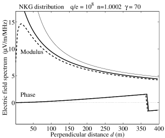
Another difference with the Coulomb field is that the phase varies rapidly with the charge energy, except at small frequencies and/or distances, since for ; hence we see from (54) that integrating over a distribution of should decrease the field strength.
7 Comparison with the Čerenkov radiation
We have seen that the electric field is essentially directed along the vector from the charge’s present position to the antenna ( axis), i.e. perpendicular to the velocity. However, it is not this field that is at the origin of conventional Čerenkov radiation, but instead the (smaller) component parallel to the velocity ( axis).
Indeed, the energy flow through a cylinder of radius around the charge’s path is given by
| (57) |
since the wave magnetic field with given by (43) is along . This integral, along the cylinder at a given time, may be transformed into an integral over time at a given point on the cylinder (using again )
| (58) |
Converting this time integral into a frequency integral, we obtain
| (59) |
where . For a point charge , is given by (42) and by (45). Using the expansions for large arguments of the Hankel functions and , we obtain the power radiated by the particle
| (60) |
which is the well-known Frank-Tamm result. If instead of a point charge, the charge is distributed round a circle of radius , we have from Eqs. (43), (48), (52), and (56)
| (61) |
with given by (40) - a result that can also be found directly using for example the general expression derived by Meyer-Vernet (mey88 (1988)) with a different formulation.
8 Discussion
8.1 Physical significance of the results
We have calculated analytically the boosted Coulomb and Čerenkov contributions to the electric field spectrum produced by an extensive cosmic ray shower, with a highly simplified model. These field contributions are due to the relativistic speed of the radiating charges and do not depend on the acceleration. The result may be understood more intuitively by using Feynman’s formula sign(), where is the retarded angular position of the particle (Fig. 1). This formula, which can be derived from the Liénard-Wiechert potentials used in the present paper (Feynman fey64 (1964)), was used by Allan (all71 (1971)) in his seminal review. With Allan’s notations (origin at when the charge passes at closest approach C), we have from Fig. 1: . The solutions for (one solution for , two solutions in the Čerenkov cone for ), and the second derivatives are given respectively in Eqs.(A16)-(A17) and Fig. A5 of the paper by Allan (all71 (1971)). This yields an electric field varying as for and as for ( being the Heaviside function), in agreement with Eqs. (9) and (41) of the present paper. Feynman’s formula is more intuitive than the Liénard-Wiechert formulation used here, but it leads to more complicated calculations for the present problem.
Feynman’s formula enlightens the fact that the boosted Coulomb and Čerenkov fields both stem from the strong acceleration of the retarded angular trajectory at relativistic speeds, even when the charge’s speed is a constant. This takes place during a short interval of time near the instant when the charge’s path (not necessarily the charge itself as we already noted, see Feynman fey64 (1964)) passes at closest approach to the antenna (if ) or has the antenna on its Čerenkov cone (if ). As already noted, the boosted Coulomb and the Čerenkov field have the same spectrum at low frequencies (), which is the time integral of the field, and is independent on both the Lorentz factor and the refractive index .
8.2 Boosted Coulomb versus Čerenkov
An important fact about cosmic ray showers is that the median speed of secondary charged particles is roughly equal to the phase speed of radio waves in air at about half the atmosphere scale height. As a consequence, roughly the lower half of the particle energy distribution produces a boosted Coulomb field, roughly the higher half produces a Čerenkov field, whereas the particles moving nearly at the wave phase speed should not contribute except at very small distances, because in that case the retarded altitude of emission (respectively (8) and (39) for the Coulomb and Cerenkov cases) jumps above the atmosphere.
The boosted Coulomb and Čerenkov field spectra of a point charge are equal at small distances and/or frequencies, but the Coulomb field decreases with frequency and distance more rapidly than the Čerenkov one. However, the Čerenkov field at large frequencies or distances is produced when the antenna is very close to the Čerenkov cone, so that it should be very sensitive to the variation of the refractive index with altitude, much more so than the boosted Coulomb field which does not involve any singularity. Furthermore, the Čerenkov field is produced by the high energy tail of the shower particles, for which the net charge and the magnetic separation are smaller. The Čerenkov field is thus expected to be smaller than the boosted Coulomb field - a question that should be examined more carefully.
Finally, we have not considered the transition radiation (see Ginzburg & Tsytovich gin79 (1979)) that may be produced by the variation in refractive index, especially when the charges hit the ground.
8.3 Comparison with synchrotron emission and with observations
The present estimate does not take into account the electric field produced by the acceleration due to the Lorentz force (see Huege & al. hue07 (2007) and refs. therein), which yields opposite (time varying) deviations of the velocities of charges of opposite signs. The field due to the acceleration by the Lorentz force has been calculated as a special case of synchrotron radiation (see Huege & Falcke hue03 (2005)) with each particle completing only a small fraction of gyration since the free path is much smaller than the gyroradius.
However, it should be noted that the published simulations of that emission neglect the effect of refraction. Taking into account the air refractive index may change the spectral density and the radiation pattern, even for particles satisfying , by introducing an “equivalent Lorentz factor” according to (10), whereas for , the charges can catch up with the waves they emit. A naive application of the classical expression of the synchrotron formulae (Jackson jac99 (1999)) would suggest that for a given charge, refraction should not change significantly the field at small frequencies or distances since in that case it does not depend on . However, refraction should change the retarded altitude of emission, and therefore the number of radiating charges, since it depends on the development of the shower. In particular, charges with have a retarded altitude above the atmosphere (except for very short perpendicular distances), and thus should not contribute to radiation.
Nevertheless, it may be interesting to compare the boosted Coulomb field with the published simulations of synchrotron radiation. We find a Coulomb field strength (see for example Fig. 7) that may not be negligible compared to the values calculated for synchrotron radiation (see Huege & al. hue07 (2007) and refs. therein). Furthermore it appears to have a spectral decrease with frequency and distance that is grossly similar; for example the scale of decrease is of the order of magnitude of 100 m at 20 MHz. More precise comparisons require further studies which are outside the scope of this paper. Note however that the boosted Coulomb and the synchrotron spectral shapes have different physical origins. The roughly exponential decrease with both frequency and lateral distance is a generic property of the boosted Coulomb field, which stems from the expansion of the Bessel function for large arguments (20), whereas the field strength tends to a finite constant (19) as . In contrast, the synchrotron electric field spectrum of a point charge does increase with frequency, with the field vanishing for , so that the field decrease with frequency exhibited by the synchrotron simulations is produced by the longitudinal extension of the source and is very sensitive to the time of arrival distribution (see Huege & Falcke hue03 (2005)).
The boosted Coulomb field strength shown in Fig. 7 is of the same order of magnitude as the published observations (see Allan all71 (1971), Ardouin ard06 (2006), Horneffer hor06 (2006), Lecacheux & al. lec07 (2007)), including the scale of variation with distance. For example Fig. 7, calculated with a plausible source size and a total number of particles (roughly proportional to the primary energy) corresponding to shower maximum development for a primary of eV, yields a low-frequency field Fourier transform of about 6 V/m/MHz at 100 m perpendicular distance, decreasing with a spatial scale of about 100 m; with the same parameters, the relative excess of electrons over positrons yields an additional field of times the value in Fig. 6. Note that the spectral densities (defined for positive frequencies only) are twice these values, and that the above estimates are only order-of-magnitude ones. Comparing with Fig. 38 of Huege & Falcke hue03 (2005) for example suggests that this contribution may not be negligible.
Finally, since the boosted Coulomb field is produced by the charges satisfying and whose retarded altitude (8) (depending on , too) is in the region of significant shower development, it depends on the refractive index. The field should thus be sensitive to atmospheric pressure, temperature, and humidity.
8.4 Defects of the model
In order to obtain analytical results, we made many simplifications which make our work little more than a preliminary step for more detailed calculations. In particular, one should take into account the variation of the refractive index with altitude, the longitudinal distribution of the source, the variation of the charge distribution with (retarded) altitude, the deviations of the particle velocities, and the particle velocity distribution. Such studies, which require a detailed numerical simulation of the shower, are outside the scope of this paper.
In particular, as indicated in Section 4, the longitudinal extent of the source should reduce the amplitude above about 50 kHz, because of loss of coherence.
In order to obtain analytical results, we have considered a fixed value of , close to the median value for shower secondaries. A realistic calculation should involve an integration over the particle velocity distribution, taking care of the singularity at . This singularity is expected to be alleviated by the fact that the corresponding retarded altitude jumps above the atmosphere, so that the charges producing it cannot contribute. Hence, at distances of hundreds of metres and frequencies of tens of MHz, the integration of the field strength over is expected to produce a result behaving roughly as calculated in Sections 3 and 4, with a value of roughly equal to the maximum value for which the retarded altitude yields a significant charge.
9 Conclusions
We have evaluated the electric field produced by the relativistic velocity of the charges in extensive cosmic ray showers, using a highly simplified model of the charge distribution in order to obtain analytical results. We show that the refractive index plays an important role, not only in producing a Čerenkov-like field at supraluminal speeds, but also in changing the emission at subluminal speeds since the bulk of secondary particles move roughly at the wave phase speed. In particular, except for small perpendicular distances, this puts above the atmosphere the retarded altitude of the particles moving close to the wave phase speed, so that they do not contribute to the field. Even though our calculations are based on oversimplified hypotheses, the analytical formulas obtained are useful to estimate the importance of various parameters and physical processes for the part of the field that does not depend on the acceleration. Our main results are listed below.
1) A little less than the lower half of the charge energy distribution in the shower produce a boosted Coulomb electric field. With plausible parameters of the charge distribution, this yields an electric field spectrum comparable to the values calculated for synchrotron radiation and to those observed. In particular, we find that a primary of eV should produce a spectral field of a few V/m/MHz at 20 MHz and 100 m perpendicular distance, decreasing roughly as an exponential with the product of perpendicular distance by frequency, with a scale of decrease of about 100 m at 20 MHz. This is comparable to current measurements, and therefore does not appear to be negligible.
2) Charges of higher energy produce a Čerenkov-like field. However, this field may be more difficult to detect for several reasons: first, the relative excess of electrons over positrons is small at these energies, making the net charge small; second, the magnetic separation between electrons and positrons decreases with energy as ; third, the phase varies with lateral position, so that the finite lateral size of the source decreases the field amplitude because of loss of coherence, except at very small frequencies; this is not the case of the Coulomb field, for which loss of coherence is only produced by the (small) longitudinal extension. And finally, it is only at large frequencies or distances () that the Čerenkov-like field may be greater than the boosted Coulomb contribution, and in this range the variation of the refractive index with altitude should play an important role.
3) The radio electric field depends on the air refractive index, and thus on the pressure, temperature and concentration of various components, especially humidity. This should introduce variations of radio emission with the altitude of emission and reception, and may produce significant day-night, seasonal and other effects.
4) This study suggests several developments which are outside the scope of this paper. In particular, taking into account the variation of the refractive index with altitude, and making a detailed comparison with synchrotron emission.
Acknowledgements.
D. Ardouin is grateful to Observatoire de Paris for hospitality and support.References
- (1) Abramowitz, M. & Stegun, I. A. 1972, Handbook of Mathematical Functions (Dover Publications, New York)
- (2) Abu-Zayyad, T. & al. 2001, Astropart. Phys., 16, 1
- (3) Allan, H. R. 1971, Prog. Element. Part. Cosmic Ray Phys., 10, 169
- (4) Antoni, T. & al. 2001, Astropart. Phys., 14, 245
- (5) Ardouin, D. & al. 2006, Astropart. Phys., 26, 341
- (6) Askar’yan, G. A. 1962, Soviet Phys. JETP, 14, 441
- (7) Birch, K. P. 1994, Metrologia, 31, 315
- (8) Clemmow, P. C. & Dougherty, J. P. 1969, Electrodynamics of Particles and Plasmas (Addison-Wesley)
- (9) Feynman, R. P. & al. 1964, The Feynman Lectures on Physics II-21, II-26 (New York, Addison-Wesley)
- (10) Ginzburg, V. L. & Tsytovich V. N. 1979, Physics Rep. 49, 1
- (11) Ginzburg, V. L. 1989, Applications of Electrodynamics in Theoretical Physics and Astrophysics (Gordon & Breach)
- (12) Horneffer, A. 2006, Ph. D Thesis, University Bonn
- (13) Huege, T. & Falcke, H. 2005, A&A, 430, 779
- (14) Huege, T. & al. 2007, Astropart. Phys., 27, 392
- (15) Jackson, J. D., 1999, Classical Electrodynamics (Wiley)
- (16) Kahn, F. D. & Lerche, I. 1966, Proc. Roy. Soc. A 289, 206
- (17) Lecacheux A. & al. 2007, unpublished manuscript
- (18) Linsley, J. 1986, J. Phys. G 12, 51
- (19) Meyer-Vernet, N. 1988, Am.J. Phys. 57, 1084
- (20) Nishimura, J. 1967, Handbuch der Physik 46/2, 1 (Springer, Berlin)
- (21) Thidé, B. 1997, Electromagnetic Field Theory (Upsilon Books, Uppsala, Sweden)
- (22) Watson, G. N. 1966, A treatise on the theory of Bessel functions (Cambridge University Press), p. 359