The Circumstellar Environment of High-Mass Protostellar Objects.
IV. C¹⁷O Observations and Depletion

Abstract

Aims. The presence of depletion (freeze-out) of CO around low-mass protostars is well established. Here we observe 84 candidate young high-mass sources in the rare isotopologues C¹⁷O and C¹⁸O to investigate whether there is evidence for depletion towards these objects.

Methods. Observations of the J $=2\rightarrow 1$ transitions of C¹⁸O and C¹⁷O are used to derive the column densities of gas towards the sources and these are compared with those derived from submillimetre continuum observations. The derived fractional abundance suggests that the CO species show a range of degrees of depletion towards the objects. We then use the radiative transfer code RATRAN to model a selection of the sources to confirm that the spread of abundances is not a result of assumptions made when calculating the column densities.

Results. We find a range of abundances of C¹⁷O that cannot be accounted for by global variations in either the temperature or dust properties and so must reflect source to source variations. The most likely explanation is that different sources show different degrees of depletion of the CO. Comparison of the C¹⁷O linewidths of our sources with those of CS presented by other authors reveal a division of the sources into two groups. Sources with a CS linewidth $>3$ km s^-1 have low abundances of C¹⁷O while sources with narrower CS lines have typically higher C¹⁷O abundances. We suggest that this represents an evolutionary trend. Depletion towards these objects shows that the gas remains cold and dense for long enough for the trace species to deplete. The range of depletion measured suggests that these objects have lifetimes of $2-4\times 10^{5}$ years.

1 Introduction

Many questions regarding the formation mechanism of high-mass stars remain unanswered. Young high-mass stars form within massive cores and display features common to low-mass star formation such as outflows and in some cases disks (e.g. Shepherd, 2005; Cesaroni et al., 2007). However the different stages through which a core forming a high-mass star evolves remains unclear.

In the cold, dense conditions within cores prior to their collapse, trace molecules freeze-out onto the dust grains forming icy mantles. This process reduces the abundances of species in the gas phase until the grains are heated, desorbing the molecules off the grains and returning them back into the gas. This freeze-out and evaporation cycle is potentially an important indicator of the age of the material in star forming cores and how the material has evolved.

The transitions of the two rare isotopologues of CO, C¹⁸O and C¹⁷O which have abundances with respect to H₂ of $\sim 2\times 10^{-7}$ and $\sim 5\times 10^{-8}$ respectively (Frerking, Langer & Wilson, 1982), are often employed to probe the inner regions of dense cores (Tafalla et al., 2002; Caselli et al., 1999; Redman et al., 2002) as their transitions are typically optically thin, especially those of C¹⁷O. A number of studies of various, but mainly low-mass, star forming regions using these species have provided evidence for depletion of CO towards the centres of cores (Caselli et al., 1999; Kramer et al., 1999; Tafalla et al., 2002; Willacy et al., 1998; Savva et al., 2003) with the degree of depletion varying from from factors of a few to over an order of magnitude compared to the canonical CO abundance.

In this paper we present new observations of candidate high-mass star forming regions in C¹⁷O and C¹⁸O made in order to look for evidence of depletion in these regions.

2 Observations of C¹⁷O and C¹⁸O

Sridharan et al. (2002, hereafter SBSMW) searched the IRAS catalogue and identified 69 point sources which represent potentially massive, deeply embedded protostars in the Galactic plane. These sources have been studied extensively by Beuther et al. (2002a, b) and have been mapped with SCUBA, the James Clerk Maxwell Telescope (JCMT) bolometer array, at 850 $\mu$m and 450 $\mu$m by Williams, Fuller & Sridharan (2004, hereafter WFS04) as well as being surveyed for evidence of infall by Fuller et al. (2005). In many cases the submillimetre and millimetre continuum maps show more than a single peak indicating multiple sites of potential star formation. In total 112 850 $\mu$m peaks were identified of which we have observed 84 in C¹⁷O.

We observed the J $=2\rightarrow 1$ rotational transitions of C¹⁸O (219.560  GHz) and C¹⁷O (224.714 GHz) towards 31 sources during May 2004 at the JCMT in Hawaii as part of observing program M04AU47. We used the RxA3 receiver with the DAS autocorrelator with channels of 78 kHz in position switching mode using a reference position of (+600^′′, +600^′′). The reference positions were chosen to be free of C¹⁸O emission having been checked and used for previous molecular observations. The pointing was checked every couple of hours. The typical zenith opacity at 225 GHz was between 0.15 and 0.4 and we achieved a typical rms of $\lesssim$0.25 K. The data were baseline subtracted using the SPECX package following normal routines.

As we are primarily interested in deriving column densities, in further observations we chose to concentrate on the C¹⁷O line which has lower optical depth. A further 53 sources were observed in C¹⁷O J $=2\rightarrow 1$ in July and August 2005 (in observing program M05BU46). In addition we observed a selection of these sources in the J $=3\rightarrow 2$ transition of C¹⁷O (337.061 GHz) with the RxB3 receiver. This time we achieved a typical rms of $\lesssim$0.15 K. These data were processed in the same way as the earlier data.

As the telescope beam is not perfectly coupled to the source it is necessary to apply a correction factor to convert antenna temperature into a main beam temperature where

$$T_{mb}=\frac{T_{A}^{*}}{\eta_{mb}}$$

At the JCMT the main beam efficiencies are 0.69 at 220 GHz with a beam size of 20^′′ and 0.63 at 337 GHz with a beam size of 13^′′. The positions and dates of observations for all the sources are given in Table 8.

3 Analysis

	C18O J $=2\rightarrow 1$				C17O J $=2\rightarrow 1$
WFS	Peak $T_{mb}$	$v_{lsr}$	$\Delta v$	$\int T_{mb}dv$	Peak $T_{mb}$	$v_{lsr}$	$\Delta v$	$\int T_{mb}dv$
	(K)	(km s-1)	(km s-1)	(K km s-1)	(K)	(km s-1)	(km s-1)	(K km s-1)
14	9.77	33.26	2.42	25.61	2.59	33.22	2.45	7.75
16	10.54	59.22	3.36	37.38	3.97	59.19	3.00	14.03
17	10.74	45.08	2.72	32.74	3.45	45.09	2.67	11.65
20	3.30	34.39	2.82	9.80	1.26	34.28	2.71	4.19
21	5.19	34.39	2.25	12.74	1.75	34.35	2.29	5.22
22	8.99	84.51	2.23	21.42	3.09	84.48	2.01	8.01
25	7.17	77.85	2.47	19.64	2.52	77.78	2.25	7.62
29	5.48	58.94	2.69	15.22	2.67	59.24	2.16	7.59
30	4.06	95.69	2.44	13.01	0.96	95.75	2.87	3.70
34	8.09	22.83	3.39	30.06	2.62	22.96	3.41	10.97
36	4.67	15.79	2.64	16.12	1.99	15.93	2.58	6.39
39	5.13	96.07	2.64	17.28	1.91	96.04	2.63	6.46
51	7.75	84.29	1.85	14.84	2.32	84.33	1.75	5.16
78	4.99	21.72	2.83	15.12	1.32	21.80	2.47	4.22
79	6.01	22.53	2.85	19.07	1.74	22.54	2.34	6.10
85	-	-	-	-	1.41	11.20	2.40	4.45
87	-	-	-	-	2.64	5.58	1.26	5.04
88	-	-	-	-	4.25	5.83	0.93	6.43
90	5.43	-3.64	2.83	17.29	1.46	-3.67	2.92	5.54
91	10.38	-1.89	1.26	14.01	3.13	-1.85	1.20	5.78
95	-	-	-	-	0.94	8.52	2.33	2.80
96	-	-	-	-	1.87	-3.19	2.01	4.89
97	-	-	-	-	1.33	-2.19	2.77	4.36
99	6.01	11.16	2.10	13.46	1.80	11.12	1.80	4.23
100	4.94	11.40	2.85	14.12	1.54	11.40	2.60	4.81
107	4.09	-45.85	2.25	10.38	1.26	-45.86	1.85	3.01
108	5.10	-53.18	2.79	16.48	1.52	-53.11	2.82	5.88
109	4.36	-44.29	2.74	13.47	1.29	-44.38	2.33	4.00
110	3.91	-54.71	2.31	10.09	1.22	-54.73	2.39	3.62
111	10.17	-17.94	1.46	15.81	3.29	-17.88	1.26	6.28
112	6.68	-18.45	1.84	12.51	1.87	-18.62	1.55	4.01

Table 1: Observed line parameters. The columns give the peak intensity, velocity, linewidth and integrated intensity for C¹⁸O  and C¹⁷O  respectively. For C¹⁷O the first three parameters are derived from hyperfine fitting of the data using CLASS. The integrated intensity was obtained using a single Gaussian fit.

	C17O J $=2\rightarrow 1$				C17O J $=3\rightarrow 2$
WFS	Peak $T_{mb}$	$v_{lsr}$	$\Delta v$	$\int T_{mb}dv$	Peak $T_{mb}$	$v_{lsr}$	$\Delta v$	$\int T_{mb}dv$
	(K)	(km s-1)	(km s-1)	(K km s-1)	(K)	(km s-1)	(km s-1)	(K km s-1)
1	1.04	-17.33	2.14	2.64	1.80	-17.42	2.06	4.56
3	1.17	0.10	1.72	3.01	1.52	0.09	1.89	3.78
4	0.57	0.80	2.40	2.35	$<$0.54	-	-	-
6	1.42	5.76	1.81	3.48	1.55	5.79	1.76	3.51
12	1.46	110.88	2.47	4.71	-	-	-	-
13	0.72	21.81	3.36	2.71	-	-	-	-
15	1.65	59.92	2.86	5.70	-	-	-	-
18	1.55	120.91	3.01	5.36	-	-	-	-
19	1.83	44.07	2.70	6.67	-	-	-	-
22	*	*	*	*	1.67	84.65	2.08	3.92
23	2.80	84.17	2.12	7.30	-	-	-	-
24	0.84	76.48	2.72	2.72	-	-	-	-
28	2.75	84.09	2.13	8.16	-	-	-	-
29	*	*	*	*	2.61	59.22	1.67	7.37
33	2.80	110.09	2.76	8.81	-	-	-	-
35	0.81	26.14	3.77	3.35	-	-	-	-
37	2.77	105.46	2.10	7.39	-	-	-	-
38	0.91	111.16	1.55	1.84	-	-	-	-
39	*	*	*	*	2.03	96.37	2.08	5.48
41	$<$0.44	-	-	-	-	-	-	-
42	0.77	98.07	2.90	2.80	-	-	-	-
51	*	*	*	*	1.25	84.52	1.25	2.49
55	0.91	49.50	3.96	5.17	-	-	-	-
57	0.71	83.47	1.99	1.84	-	-	-	-
58	1.58	82.75	4.25	7.80	-	-	-	-
59	1.22	76.42	2.56	3.87	-	-	-	-
60	$<$0.46	-	-	-	-	-	-	-
61	1.99	76.87	2.72	6.55	-	-	-	-
62	$<$0.36	-	-	-	-	-	-	-
63	0.12	50.64	1.42	0.86	-	-	-	-
64	1.28	10.40	3.22	4.75	-	-	-	-
66	2.41	66.13	3.05	9.04	-	-	-	-
67	1.01	32.62	3.17	3.96	-	-	-	-
68	1.28	55.09	2.38	4.14	-	-	-	-
69	0.85	54.54	2.39	2.20	-	-	-	-
70	0.91	6.54	1.82	2.55	-	-	-	-
71	0.87	14.17	2.93	3.14	-	-	-	-
72	1.07	3.77	3.94	4.86	-	-	-	-
74	0.96	4.82	3.34	3.77	-	-	-	-
75	2.93	23.09	1.45	5.97	-	-	-	-
76	2.74	24.04	1.18	4.75	-	-	-	-
77	2.81	26.66	1.05	4.20	5.03	26.72	0.89	6.14
78	*	*	*	*	1.12	21.49	2.32	3.14
79	*	*	*	*	1.93	22.45	2.26	5.86
80	1.55	28.86	1.85	3.90	2.10	29.01	1.86	4.97
81	1.99	20.29	1.69	4.38	1.17	20.43	0.94	2.63
82	3.13	20.06	1.81	7.77	4.23	19.96	1.48	8.02
83	0.94	21.47	1.66	2.43	0.97	21.60	1.40	1.95
84	1.19	22.32	2.01	3.55	1.42	22.54	1.49	2.54
86	0.87	5.72	1.94	2.55	-	-	-	-
89	0.80	5.47	0.92	1.04	-	-	-	-
90	*	*	*	*	1.49	-3.48	3.10	6.52
91	*	*	*	*	4.96	-1.89	1.10	7.81
92	0.83	-1.69	1.63	1.88	-	-	-	-
93	1.48	-1.69	1.60	3.57	-	-	-	-
94	1.36	6.03	2.61	4.13	-	-	-	-
98	1.83	11.50	1.03	2.90	-	-	-	-
101	1.81	-18.38	1.81	4.41	-	-	-	-
102	$<$0.65	-	-	-	-	-	-	-
103	$<$0.69	-	-	-	-	-	-	-
104	1.52	-12.35	0.95	2.38	-	-	-	-
107	*	*	*	*	1.83	-45.97	1.57	3.75
108	*	*	*	*	1.51	-53.21	2.70	5.03
109	*	*	*	*	1.49	-44.37	2.58	4.83
110	*	*	*	*	1.80	-54.75	2.00	4.67
111	*	*	*	*	4.77	-17.84	1.09	7.00
112	*	*	*	*	3.13	-18.59	1.24	4.95

Table 2: Observed line parameters. The columns give the peak intensity, velocity, linewidth and integrated intensity for C¹⁷O. The first three parameters are derived from hyperfine fitting of the data using CLASS. The integrated intensity was obtained using a single Gaussian fit. Three sigma upper limits are shown for sources where a line was not detected above this threshold. An * indicates an data that has been been observed in the previous year and is given in Table 1.

3.1 Line Profiles

The line parameters were initially measured using SPECX by fitting Gaussian line-profiles to derive the source velocity ($v_{lsr}$), line width ($\Delta v$), peak line flux ($T_{A}^{*}$) and integrated line intensities.

All the C¹⁸O data were fitted with a single Gaussian. These fits produced typical peak temperatures of $T_{A}^{*}\sim 2.5-7.5$ K, and linewidths of $\Delta v\sim 1.5-3.5$ km s^-1. However examination reveals that a significant fraction of these C¹⁸O data ($\sim$65%) are distinctly better fit, with smaller residuals, by the sum of two different velocity components. The results of two components fits are also given in Table 7. Those sources with multiple components can be divided into two categories; those where the 2 components are of approximately equal width, but are offset in velocity, and those where there is a definite separation into a broad and a narrow component, with the broad component possibly being a related to the outflow from the source. In this latter case the typical linewidths of the broad and narrow components are $\Delta v_{br}\geq 3$ km s^-1 and $\Delta v_{n}\leq 2$ km s^-1.

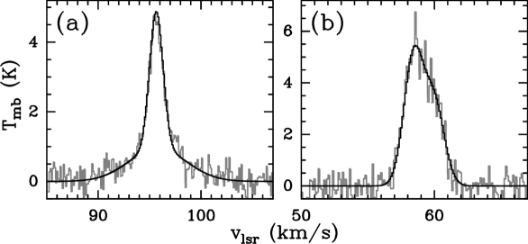
Figure 1: Example spectra of C¹⁸O line profiles for (a) WFS30 and (b) WFS29 which are best fit by 2 Gaussian components shown as the smooth curve over each line.

The integrated intensities for C¹⁷O have been calculated from a Gaussian fit using SPECX. However unlike the C¹⁸O, the transitions of C¹⁷O have hyperfine structure. Simple Gaussian fits to the C¹⁷O data therefore overestimate the intrinsic velocity dispersion. The C¹⁷O line parameters were therefore fitted with the known hyperfine structure (hfs) of the respective transitions using METHOD HFS in the CLASS package assuming all components have equal excitation temperatures. For the J $=2\rightarrow 1$ transition there are 9 hyperfine components, while there are 14 for the J $=3\rightarrow 2$ transition. The line parameters, the peak intensity, the $v_{lsr}$, the linewidth and the integrated intensity are given in Tables 1 and 2. The optical depths calculated from the hfs fits imply these sources are optically thin in C¹⁷O with $\tau\sim 0.1$.

3.2 Ratio of Integrated Intensities

The ratio of C¹⁸O to C¹⁷O line intensities can constrain the optical depth of the line if the abundance ratio is known (Ladd, Fuller & Deane, 1998). Penzias conducted a survey of 15 massive star forming regions lying in the galactic disk (Penzias, 1981) and derived a value of R = [¹⁸O]/[¹⁷O] = 3.65 $\pm$ 0.15 and found no gradient based on galactocentric distance. Further work by different authors have produced values, assuming that [C¹⁸O]/[C¹⁷O] = [¹⁸O]/[¹⁷O], ranging from R = 2.9 $\pm$ 1.2 (Sheffer et al., 2002) to 4.15 $\pm$ 0.52 (Bensch et al., 2001). More recently Ladd (2004) conducted a survey of 648 lines of sight towards 5 star forming regions in the Taurus molecular cloud and combining the results for the individual regions concluded that R = 4.0 $\pm$ 0.5, a value consistent with an analysis of other clouds by Wouterloot, Brand & Henkel (2005).

A comparison of our measured C¹⁷O and C¹⁸O integrated intensities is shown in Figure 2. Assuming equal excitation temperatures and beam filling factors for the two species, if the emission is optically thin one would expect the ratio of the integrated line intensity of the two species to equal the abundance ratio. A standard value of 3.65 for the abundance ratio of C¹⁸O to C¹⁷O is indicated by the solid line. Of the sources, 5 lie approximately on the line implying that for the C¹⁸O and C¹⁷O lines are optically thin. The absence of any sources above the line is consistent with both the abundance ratio values of Penzias (3.65) and Ladd (4.0), but not higher values. As so many of our sources lie close to this line it suggests that the value of 3.65 is the upper limit for this ratio. However, the majority of our sources lie below this value suggesting that the C¹⁸O emission is not optically thin. The figure also shows the expected ratio of integrated intensities for optical depth 2 in the C¹⁸O transition. Due to the overlap of the hyperfine components of the C¹⁷O  the optical depth at the line peak depends on the velocity dispersion. The line on the figure has been calculated for a FWHM velocity of 3 km s^-1 (and a C¹⁸O to C¹⁷O abundance ratio of 3.65) giving a corresponding C¹⁷O peak optical depth of 0.5. If the FWHM velocity was 1 km s^-1, the C¹⁷O optical depth would be reduced by a factor of 0.67, whereas if the the FWHM velocity was 5 km s^-1, the optical depth would be increased by a factor of 1.05. The figure shows that the C¹⁷O emission is not highly optically thick towards these sources, a result consistent with optical depth implied by the fit to the hyperfine structure of the observed lines (Sec. 3.1). The figure also shows that there is no correlation between line strength and optical depth.

Figure 2: Comparison of the integrated intensities of C¹⁸O and C¹⁷O. The solid line denotes an abundance ratio of C¹⁷O to C¹⁸O of 3.65, the expected value if both lines are optically thin (Penzias, 1981; Ladd et al., 1998). The dotted line indicates the best-fit curve of 2.8. The dashed line indicates an optical depth of 2 associated with C¹⁸O

3.3 Column Densities

Since the C¹⁷O emission appears to not be optically thick, we calculate the column densities assuming that the C¹⁷O is optically thin. This is consistent with the analysis of C¹⁷O towards similar objects by both van der Tak et al. (2000) and Fontani et al. (2006).

To calculate the CO column densities we used the following general expression assuming LTE and optically thin emission;

$$N_{tot}=\frac{3k}{8\pi^{3}\nu\mu^{2}g_{u}}\frac{Q(T_{ex})}{\exp(-E_{u}/kT_{ex})}\int T_{mb}dv$$

Here $g_{u}$ is the statistical weight, $Q(T)$ is the partition function and $\mu$ is the electric dipole moment for that molecule. Expressing the integrated intensity in K km s^-1, the dipole moment in Debye ($\mu$=0.11 D for CO) and the frequency in GHz, this reduces to

$$N_{tot}=1.67\times 10^{14}\frac{Q(T_{ex})}{\mu^{2}({\rm Debye})\nu({\rm GHz})g_{u}}\exp\left(\frac{E_{u}}{T_{ex}}\right)\int T_{mb}dv$$

This method assumes a constant excitation temperature ($T_{ex}$) along the line of sight which is a free parameter in the analysis. For all their observed sources, SBSMW also estimated the temperature of the cold component of the dust; the mean over the whole sample was 45 K. SBSMW also measured the gas temperature towards many of the sources observed here using NH₃. Over their entire sample SBSMW find a mean temperature of 19 K and for all but two of the sources observed here they found temperatures of $<20$ K. To estimate the C¹⁷O column density we have adopted 30 K, a compromise value intermediate between cold dust and NH₃ temperatures. The column density is of course sensitive to the assumed excitation temperature and is at a minimum at $T_{ex}$= 17 K. At 10 K and 30 K the column densities are approximately equal and about 16% higher than at the minimum.

For comparison with the observations of the dust towards the sources it was necessary to re-convolve the 850 $\mu$m data to a beamsize to match that of the CO beam. We first calculate the mass in the beam using the expression

$$M_{(beam)}=\frac{S_{\nu(beam)}d^{2}}{\kappa_{\nu}B_{\nu}(T_{dust})}$$

where we take the value for the opacity from WFS04 as $\kappa_{850}$=1.54$\times$10^-2 cm²g^-1 and the dust temperature (T_dust) as the cold dust component given in SBSMW. We then derive the beam-averaged hydrogen column density from the submillimetre mass using the relationship from Hildebrand (1983) given as

$$M_{(beam)}=[\pi\theta^{2}_{\frac{1}{2}}d^{2}]N(H+H_{2})m_{H}\mu$$

where $m_{H}$ is the mass of a hydrogen atom and $\mu$ is the ratio of total gas mass to hydrogen mass and $\theta_{\frac{1}{2}}$ is the beam radius. In both steps the distance to the source, $d$, is taken to be the near-distance if there is an ambiguity (SBSMW). The results for $N$(C¹⁷O) are given along with the hydrogen column density derived from the dust continuum emission in Table 3.

	N(C17O)	N(C17O)	N(H2)	$\frac{\rm{N(C^{17}O}\ 2-1)}{\rm{N(H_{2})}}$		N(C17O)	N(C17O)	N(H2)	$\frac{\rm{N(C^{17}O}\ 2-1)}{\rm{N(H_{2})}}$
WFS	J $=2\rightarrow 1$	J $=3\rightarrow 2$			WFS	J $=2\rightarrow 1$	J $=3\rightarrow 2$
	($\times$1015)	($\times$1015)	($\times$1022)	($\times$10-8)		($\times$1015)	($\times$1015)	($\times$1022)	($\times$10-8)
1	0.64	0.90	4.03	1.58	68	1.00	-	2.86	3.50
3	0.73	0.74	2.87	2.53	69	0.53	-	-	-
4	0.57	0.00	2.38	2.38	70	0.62	-	1.90	3.24
6	0.84	0.69	3.57	2.35	71	0.76	-	3.34	2.27
12	1.14	-	4.16	2.73	72	1.21	-	9.64	1.25
13	0.65	-	10.01	0.65	74	0.91	-	6.97	1.31
14	1.87	-	8.15	2.30	75	1.44	-	5.96	2.42
15	1.37	-	1.62	8.47	76	1.15	-	2.03	5.66
16	3.39	-	12.09	2.80	77	1.01	1.21	2.11	4.81
17	2.81	-	4.96	5.67	78	0.98	0.62	3.60	2.72
18	1.29	-	6.09	2.13	79	1.33	1.15	12.15	1.10
19	1.61	-	23.25	0.69	80	0.94	0.98	4.09	2.30
20	1.01	-	0.98	10.28	81	1.06	0.52	1.80	5.87
21	1.26	-	1.20	10.47	82	1.88	1.58	3.06	6.13
22	1.93	0.77	5.53	3.50	83	0.59	0.38	1.54	3.81
23	1.76	-	-	-	84	0.86	0.50	1.62	5.29
24	0.66	-	2.50	2.63	85	1.07	-	2.53	4.25
25	1.84	-	7.81	2.36	86	0.54	-	1.00	5.43
28	1.97	-	4.31	4.57	87	1.22	-	2.73	4.47
29	1.66	1.45	3.06	5.99	88	1.64	-	2.73	6.01
30	0.89	-	4.44	2.01	89	0.25	-	0.91	2.77
33	2.13	-	6.13	3.47	90	1.34	1.29	8.40	1.59
34	2.65	-	4.31	6.15	91	1.40	1.54	2.53	5.52
35	0.81	-	6.13	1.32	92	0.50	-	1.34	3.74
36	1.54	-	3.24	4.76	93	0.86	-	2.91	2.96
37	1.78	-	3.47	5.15	94	1.00	-	6.77	1.47
38	0.43	-	2.33	1.85	95	0.68	-	1.15	5.88
39	1.56	1.08	3.63	4.30	96	1.23	-	3.60	3.42
41	-	-	0.08	-	97	1.06	-	2.86	3.71
42	0.68	-	0.87	7.74	98	0.70	-	-	-
51	1.25	0.49	1.36	9.17	99	1.02	-	5.28	1.93
55	1.25	-	3.28	3.18	100	1.16	-	-	-
57	0.44	-	2.66	1.67	101	1.06	-	3.29	3.24
58	1.88	-	7.69	2.45	102	-	-	-	-
59	0.93	-	3.86	2.42	103	-	-	2.31	-
60	-	-	0.78	-	104	0.57	-	1.38	4.15
61	1.58	-	5.82	2.72	107	0.73	0.74	2.88	2.53
62	0.24	-	1.11	2.18	108	1.43	0.99	6.66	2.13
63	0.21	-	0.47	4.35	109	0.97	0.95	7.75	1.25
64	1.15	-	4.05	2.83	110	0.87	0.92	2.69	3.26
66	2.18	-	2.86	3.83	111	1.51	1.38	2.67	5.68
67	0.96	-	6.31	1.51	112	0.97	0.98	2.67	3.64

Table 3: Column densities calculated from the line intensities with an average rms of $\sim$0.2 K. The hydrogen column density corresponds to a 20^′′ beam to directly compare with the J $=2\rightarrow 1$ transitions of each isotope.

Figure 3 shows the column density C¹⁷O plotted against that calculated for H₂ from the dust continuum emission. Also shown are lines of constant CO abundance chosen to constrain the data. It is immediately evident that these graphs show a large scatter in the abundances. The C¹⁷O data are constrained by abundances of $\sim$1$\times$10^-7 and $\sim$7$\times$10^-9, a factor of approximately fourteen spread in the abundance. Taking the standard [C¹⁷O]/[H₂] abundance to be 4.7$\times 10^{-8}$ (Frerking et al., 1982), we would expect our sources to lie either on this line or below it in the case of CO depletion, yet it is clear that this value does not represent the upper limit for our sources and a significant fraction lie up to a factor of 2 above this line.

To explore the reliability of the derived C¹⁷O abundances, we have also run detailed models of the emission expected from these sources. These models allow us to investigate the possible consequences of some of the assumptions made when calculating the column densities, particularly the assumed excitation temperature and dust temperature, together with the role of density gradients within the beam.

Figure 3: Comparison of the column density C¹⁷O with the H₂+H column density derived from the dust continuum emission. Typical uncertainties are shown in the lower right corner of the panel. The dashed lines represent lines of constant abundance: Short dashed = 5$\times$10^-7, dot-dashed = 1$\times$10^-7, long dashed = 5$\times$10^-8 & dotted = 1$\times$10^-8. The circled sources indicate those which have been modelled (see Sec.4).

4 Modelling

To model the emission of C¹⁷O and C¹⁸O we used the 1D radiative transfer code RATRAN developed by Hogerheijde & van der Tak (2000). RATRAN utilises the Monte Carlo method to calculate the radiative transfer of molecular lines through a dusty shell.

Williams, Fuller & Sridharan (2005, hereafter WFS05) modelled the 850 $\mu$m emission for a selection of the sources observed by WFS04 using the 1D radiative transfer code DUSTY (Ivezić, Nenkova & Elitzur, 1999) in order to determine the physical parameters of the envelopes around the central embedded sources. Of those sources for which we have both C¹⁷O and C¹⁸O data, 14 were successfully modelled by WFS05. We have utilised the parameters of the best-fit models from WFS05 to generate the input for RATRAN.

WFS05 identified certain sources as asymmetric and used radial slices to explore the structure in various directions, as a result four of our 14 sources actually have multiple models in WFS05. For these sources we correspondingly generated multiple models for RATRAN. These are indicated by alphabetical suffixes to the source names.

As RATRAN is a 1D code it models the sources as spherically symmetric and hence neglects any openings or elongations due to outflows or winds. The model assumes a dust-free cavity surrounding the star from radius $r=0$ to $r=r_{1}$. Between $r_{1}$ and $r_{2}$ lies the envelope to be modelled. We divided the radial distance between r₁ and r₂ into 30 logarithmically spaced shells to give increased resolution towards the inner region of the shell where the temperature and density profiles change most rapidly. Thirty shells were used corresponding to the number used by van der Tak et al. (2000, hereafter VVEB) in their RATRAN modelling of massive young stars. We also ran a number of identical models using both 15 and 60 shells and found a negligible effect on the output compared to the 30 shell models.

To determine the input for RATRAN we used the following parameters derived in WFS05: power-law index ($\alpha$) of the envelope density profile $n(r$) where $n\propto r^{-\alpha}$, the temperature at the inner boundary $T_{1}$, the scale of the envelope defined by the inner radius, $r_{1}$ and $Y$, where $Y$ is the ratio between $r_{2}$ and $r_{1}$. The outer radius can then be calculated from $r_{2}=Yr_{1}$.

WFS	$r_{1}$	$r_{2}$	$\alpha$	$n(r_{1})$	$\Delta v$(C17O)	$\Delta v$(C18O)
	1016cm	1018cm		106cm-3	km s-1	km s-1
14	3.02	1.51	1.5	3.09	2.84	2.21
16	4.06	4.06	2.0	8.74	3.35	2.95
25	2.69	5.39	1.5	1.33	2.64	2.20
29	2.27	1.59	1.0	0.48	2.59	2.17
30	0.23	1.84	1.0	4.41	2.37	2.27
34a	1.84	0.18	1.0	32.97	3.71	3.30
34b	0.63	5.04	1.5	2.19	3.71	3.30
36	0.45	0.90	1.0	0.83	2.94	2.32
79	2.41	1.21	1.5	6.78	2.71	2.33
90a	1.78	1.25	1.5	3.44	3.27	2.87
90b	1.83	1.83	2.0	12.74	3.27	2.87
107	3.50	2.45	0.5	0.05	2.24	1.59
108a	0.64	2.56	1.5	8.35	3.25	2.83
108b	0.22	3.52	1.0	1.07	3.25	2.83
109	0.23	3.68	1.5	33.80	2.54	2.00
110a	0.64	2.56	1.5	5.19	2.82	2.09
110b	1.70	3.40	1.5	0.80	2.82	2.09
110c	1.83	1.83	2.0	16.68	2.82	2.09

Table 4: Parameters used in the detailed modelling of the sources. Where $r_{1}$ is the inner radius of the modelled envelope, $r_{2}$ is the outer radius and $\alpha$ is the power-law index of the number density profile $n(r)$ where $n\propto r^{-\alpha}$. Column 5 gives the hydrogen number density at $r_{1}$.

Figure 4: Comparison of the C¹⁷O J $=2\rightarrow 1$ (upper spectra) and C¹⁸O  J $=2\rightarrow 1$ (lower spectra) spectra with the results of the best fit results of the RATRAN models (solid curves). The model parameters are given in Tables 4 and 5.

We generated the density profile for each model by combining the power-law index ($\alpha$) of the envelope density profile given in WFS05 with the density at $r_{1}$ which we calculate from the 850 $\mu$m mass and volume of the envelope (WFS04). As the dust temperature profile is not given in WFS05 we regenerated the WFS05 models using DUSTY to determine the individual temperature profile for each model. This profile was then interpolated to the radii of the 30 shells used to trace the envelope. Given the high densities in these regions we have assumed that the gas kinetic temperatures and the dust temperatures are equal.

The turbulent line widths were taken from Gaussian fits of the optically thin C¹⁷O data. The presence of hyperfine structure for the C¹⁷O was neglected for the models. By fixing the linewidth from our observations we were able to isolate the CO abundance relative to hydrogen as the free parameter. For simplicity we restricted our models to a simple uniform abundance of C¹⁷O throughout the envelope of each source. The input parameters for each model are given in Table 4.

These parameters were then used in conjunction with the adopted collisional rate coefficients of Flower (2001) (see also Schöier et al., 2005) to generate the predicted line emission. The C¹⁷O abundances were adjusted to produce the best match to the observed C¹⁷O line profiles. The modelled sources are circled in Figure 3, illustrating that they cover a range dust and gas column densities and a range of implied C¹⁷O abundances.

The output spectra from RATRAN were continuum subtracted and convolved with a Gaussian with a FWHM equal to the appropriate JCMT beam for comparison with the observations. We analysed the quality of the models by using the reduced $\chi^{2}$ method, aligning the central channel of the model spectra with the peak of the Gaussian fit for the data. Figure 4 compares the observations with the results of the best fit models.

4.1 Modelling Results

Figure 5 shows the success with which these (simple) models can match the observed C¹⁷O line profiles and also the sensitivity of the fit to the assumed C¹⁷O abundance. In this case the C¹⁷O abundance is constrained within the noise level of the observations to within $\sim 10$%.

Since RATRAN calculates the continuum emission in parallel with the line emission it was possible to check on the consistency of the models by comparing the predicted 850 $\mu$m flux with that measured. This is especially important in this work where we are looking at the ratio of the line to continuum emission. For a number of sources modelled the predicted and measured 850 $\mu$m flux differed by more than a factor of 3. This is not completely surprising as the best fit models of WFS05 were selected to provide the best overall fit to the source SED and 850 $\mu$m distribution, as such they do necessarily provide excellent fits to the 850 $\mu$m flux alone. Therefore we have only considered the 8 sources where the predicted 850 $\mu$m continuum emission differs from the measured value by less than a factor of 3. The results of these sources are given in Table 5.

4.1.1 C¹⁷O Analysis

A comparison between the observed line profiles and the best fit model results for all the modelled sources is shown in Figure 4. The models can successfully match the observed C¹⁷O line profile with a reasonable range of C¹⁷O fractional abundances ranging over the sample from 1.8$\times$10^-8 to 1.5$\times$10^-7. Importantly for the analysis of the sources for which models of the continuum emission do not exist, comparison of the C¹⁷O abundance inferred by the modelling and that derived directly from the observations agree within a factor of $\sim$2 (Table 5). This result indicates that the assumptions made in directly estimating the C¹⁷O abundance from the observations are not overly biasing the results.

Figure 5: The observed C¹⁷O J $=2\rightarrow 1$ emission towards WFS14 overlaid with the results of three models. The only difference between the three models is the assumed C¹⁷O abundances of 5$\times 10^{-8}$, 5.5$\times 10^{-8}$ & 6$\times 10^{-8}$. The abundance is constrained within the noise level of the observations to within $\sim$10%.

4.1.2 C¹⁸O Analysis

For completeness we also attempted to model the C¹⁸O lines for the sources modelled in C¹⁷O. Initial modelling of the C¹⁸O lines involved taking the best-fit C¹⁷O abundance and scaling it up by a range of potential values of the C¹⁸O to C¹⁷O abundance ratio; these were R$=$2.8, 3.65, 4.0 & 4.5 (as mentioned in Sec. 3.2). All other free parameters remain constant with the exception of the velocity dispersion which was adopted from the C¹⁷O hfs fit (as the best estimate of the intrinsic velocity dispersion within these regions). The results are also shown in Figure 4. On inspection it is clear that a number of the models suffer from high optical depths, resulting in a flattening and broadening of the line shape, which is not seen in the observations. The inconsistencies between the data and the models for this isotopologue is perhaps not unexpected given the two velocity component profiles towards many of the sources which suggest that more than a simple envelope is contributing to the line profile.

An example of such a scenario would be a central core (as represented in our models), but surrounded by an extended low density envelope with the C¹⁸O having different optical depths in the envelope and in the core. The success of modelling the C¹⁷O from the core (Sec. 4.1) would suggest that the core has the higher optical depth.

For sources with two component C¹⁸O line profiles (Table 7), the C¹⁷O line is often intermediate in width between the two C¹⁸O components. This could also point towards the presence of two different components of material. If there are indeed two components then the simple column density analysis and model are actually overestimating the actual C¹⁷O and C¹⁸O column densities in the core, as some of the column density attributed to the core in a single component model is actually associated with the second component. This suggests that the abundances of these species in the core could be even lower than the values derived here indicate.

It is possible to test this prediction with maps of these sources; C¹⁸O emission extending beyond the detected 850 $\mu$m emission would provide evidence for an outer envelope. It is possible that the relatively small chopper throw of the 850 $\mu$m observations may have artificially removed this component from the SCUBA observations. For some sources this resulting underestimation of dust emission could account for the high abundances seen towards a few sources.

WFS	f(C17O)	$\chi^{2}_{red}$	[18O]/[17O]	R(H2)	R(C17O)
	($10^{-8}$)
14	5.2	1.69	4.0	1.36	1.35
16	10.1	1.52	4.0	1.70	2.16
29	10.0	1.79	2.8	0.76	1.00
30	5.0	1.09	4.5	2.86	1.49
36	15.0	1.58	4.5	1.30	1.88
79	1.8	2.38	3.65	0.98	0.98
90a	4.5	0.84	3.65	2.64	1.69
90b	4.5	0.86	3.65	2.15	1.69
107	4.0	1.13	2.8	1.04	0.94

Table 5: Parameters of the best fit RATRAN models. Column 2 is the fractional abundance of C¹⁷O required for the model to match the observed J $=2\rightarrow 1$ line profile. Column 3 is the reduced $\chi^{2}$ between the observed C¹⁷O J $=2\rightarrow 1$ transition and the modelled emission. R(H₂) is the ratio of measured 850 $\mu$m flux to that generated by RATRAN. R(C¹⁷O) is the ratio of the best fit abundance from the modelling to the abundance derived from comparing the data to the 850 $\mu$m hydrogen abundance: [C¹⁷O/H₂]_mod/[C¹⁷O/H₂]_data. Column 4 presents the best fit ratio of C¹⁸O/C¹⁷O  needed to match the C¹⁸O observations, scaling up the best-fit C¹⁷O abundances listed. The model line profiles are compared with the observations in Figure 4.

5 Discussion

The determination of the C¹⁷O column densities and hence abundances contain a number of sources of uncertainty. Since both the C¹⁷O lines are detected with good signal to noise ratios (Table 1; Figure 4), and the dust continuum fluxes of the sources are well measured (WFS04), the statistical uncertainties due to noise are small. The calibration uncertainties may be larger, but are likely to affect all the sources equally. However the results do also depend on a number of other assumptions. Ideally all the sources observed should be modelled in detail to determine their C¹⁷O abundance throughout their envelopes and cores. However temperature and density profiles are not (yet) available for all the objects, so this is not currently practical. Nevertheless the objects which have been modelled in detail do suggest that systematic issues do not dominate the results. The similar C¹⁷O abundances derived from the modelling of a subsample of the sources which span a range of source properties and the C¹⁷O abundances derived directly from the observations, suggests that despite the approximations and assumptions it requires, the direct derivation produces reasonable estimates of the average C¹⁷O abundance towards the sources. It is these abundances on which we will focus.

To determine the origin of the scatter seen in Figure 3 we must investigate the possible causes ranging from underlying physical differences to the simplifying assumptions. The consistency within a factor of 2 of the C¹⁷O abundances generated using RATRAN and those derived straight from the data suggests that the scatter between the observed C¹⁷O column density and H₂ column density is not a result of an overly simplistic data analysis or the assumed excitation temperature.

It is important to recognise that the hydrogen column density derived from the dust emission suffers from uncertainties due to the assumed dust properties. In calculating the dust column density we have adopted a constant value of $\kappa$, the dust mass opacity, for all the sources. For our calculations we adopted a value from Ossenkopf & Henning (1994) assuming a gas density of 10⁶ cm^-3, with thin ice mantles and 10⁵ years of coagulation. However we investigated the influence of this assumption by recalculating N(H₂) for the full range of possible opacities from Ossenkopf & Henning. By manipulating the opacity it is possible to move the entire sample in Figure 3 to a range either above the canonical C¹⁷O abundance of 4.7$\times$10^-8 or below it. However assuming that all the sources should lie at this value, it is clear that changing the dust in order to allow that to happen would have to be done on a source by source basis and utilising the full range of potential opacities.

For those sources that lie to the left of the canonical abundance line, an opacity corresponding to grains that have not undergone any coagulation would need to be adopted. This lack of grain coagulation would seem to imply that these sources, and the dust surrounding them, are young, not yet having had time for the dust to coagulate. To the other side of the line lie the sources which appear to be the most depleted of our sample. To change their abundances would require an opacity corresponding to some degree of coagulation and for the most under-abundant sources this would need to include an absence of ice mantles. The scenario of coagulated grains without ice would be consistent with the dust close to a star which has heated its surroundings and evaporated all icy mantles. However the temperature profiles derived by DUSTY modelling show that only a small part of the envelopes are this warm, with the bulk of each envelope lying at temperatures below 50 K. Under these conditions we would consider the complete absence of ice mantles to be an unreasonable assumption. The dust models indicate if mantles of any kind are present, they would limit the change in the inferred hydrogen column density to not more than 12% of the calculated values.

In addition, van der Tak et al. (1999) found that by comparing the dust mass from FIR and submm data to the gas mass derived from regions without depletion of C¹⁷O, only the opacities for dust grains with ice mantles reproduced the standard dust-to-gas ratio of 1:100. Additionally figure 3 shows a number of the sources having abundances in excess of 4.7$\times 10^{-8}$, which if not due to particular circumstances for these objects, could indicate that for the sample as a whole the hydrogen column density could be underestimated. Given these points we conclude that the scatter seen between the abundances does indeed reflect physical differences between the sources.

In principle selective photodestruction of the C¹⁷O in the inner regions of the sources close to the central heating sources could give rise to the varying C¹⁷O abundance. However selective photodestruction can only be an issue in the region up to optical depth $\sim 1$ in the UV from the inner edge of the circumstellar envelope. Although this optical depth can be contributed by either dust or line self-shielding, since the circumstellar envelopes are dusty, it is the dust that will be the dominant UV opacity source. This UV opacity corresponds to a visual optical depth $\sim 0.1$ in the optical. Since this corresponds to about 1% of the thickness of the envelope (WFS04), the internal UV flux can not be affecting the C¹⁷O abundance by more than $\sim 1$%.

The low optical depth of the C¹⁷O transitions suggest that if C¹⁷O is uniformly abundant throughout each source, the C¹⁷O emission, and hence C¹⁷O column density should, like the dust emission, trace the total column density even though the C¹⁷O has a relatively low critical density.

The most likely explanation for the variation in the C¹⁷O abundance appears to be that it reflects different gas phase abundance of C¹⁷O due to its freeze out onto dust grains. Such depletion of C¹⁷O (and by implication, CO and possibly other species) towards similar high mass sources has been previously reported by VVEB and Fontani et al. (2006).

WFS	$\overline{T}_{mw}$	WFS	$\overline{T}_{mw}$	WFS	$\overline{T}_{mw}$	WFS	$\overline{T}_{mw}$
6	23.2	19	23.5	66	26.5	95	29.7
13	25.4	25	18.6	78	18.6	107	35.3
14	28.5	29	34.1	79	28.4	108	20.8
16	23.4	30	23.4	80	27.9	109	18.4
18	18.6	36	30.0	90	25.4	110	20.8

Table 6: Mass-weighted temperatures in Kelvin, calculated for those sources for which the data are available.

5.1 Depletion of C¹⁷O

If the scatter in the C¹⁷O abundance is indeed due to depletion, then one might expect that the regions with the coolest dust would have the highest depletion. VVEB investigated this using the mass-weighted temperature, $\overline{T}_{mw}$, to define a characteristic temperature for each source.

Figure 6 shows the C¹⁷O abundance against the mass-weighted temperature for all the sources for which the necessary parameters were available. The mass-weighted temperature is defined by VVEB and was calculated here using the temperature profile from the DUSTY modelling of the sources. The figure shows data points from both our sources and those from VVEB. The two data sets are in reasonable agreement, with the distribution of both being consistent with depletion at low temperatures. The Spearman correlation coefficient indicates that the C¹⁷O abundance and mass-weighted temperature are correlated at a 96% confidence level.

We do however see a number of our sources exhibiting higher abundances at lower temperatures than VVEB, but none with showing the reverse. This is consistent with an absence of depletion at higher temperatures, whilst the sources at low temperature and high abundance could be explained by having additional contributions of C¹⁷O for regions outside the modelled core. This would be consistent with the C¹⁷O linewidths lying intermediate between the two components of the C¹⁸O lines as discussed above.

Figure 6: C¹⁷O (J $=2\rightarrow 1$) abundance against the mass-weighted temperature, $\overline{T}_{mw}$. The solid dots denote our data whilst the circles represent the data from Figure 11 in VVEB.

	C17O J $=2\rightarrow 1$				C18O J $=2\rightarrow 1$
WFS	$\Delta v$(Gauss)	$v_{lsr}$	$\Delta v$(hfs)	$v_{lsr}$	$\Delta v$(Gauss)	$v_{lsr}$	$\Delta v$(narrow)	$v_{lsr}$	$\Delta v$(broad)	$v_{lsr}$
14	2.84	33.26	2.44	33.22	2.42	33.26	2.14	33.21	3.31	33.47
16	3.35	59.21	2.99	59.19	3.36	59.22	2.43	60.40	2.46	58.63
17	3.02	45.12	2.65	45.09	2.72	45.08	2.20	44.87	3.70	45.67
20	2.99	34.35	2.70	34.29	2.82	34.39	1.60	34.99	2.97	34.03
21	2.76	34.40	2.25	34.35	2.25	34.39	1.97	34.46	3.94	33.61
29	2.59	59.28	2.18	59.28	2.69	58.94	1.83	58.42	1.93	59.93
30	3.05	95.64	2.96	95.75	2.44	95.69	1.46	95.65	5.80	95.79
39	3.08	96.07	2.61	96.03	2.64	96.07	1.55	96.36	3.72	95.53
78	2.82	21.84	2.47	21.80	2.83	21.72	0.84	21.70	3.10	21.73
79	2.91	22.60	2.33	22.54	2.85	22.53	1.30	22.49	3.96	22.66
90	3.25	-3.63	2.94	-3.67	2.83	-3.64	1.28	-3.89	3.59	-3.41
108	3.06	-53.06	2.87	-53.10	2.79	-53.18	1.50	-53.06	4.16	-53.37
109	2.56	-44.35	2.33	-44.38	2.74	-44.29	1.80	-44.58	3.57	-43.82
110	2.97	-55.00	2.09	-54.74	2.31	-54.71	1.35	-54.66	3.41	-54.24
112	2.03	-18.53	1.55	-18.62	1.84	-18.45	1.18	-17.41	1.31	-18.65

Table 7: All columns (except column 1) in units of km s^-1. The Gaussian linewidths were obtained using SPECX, whilst the hyperfine linewidths were obtained using the hfs method in CLASS. Multiple Gaussian components are only given for those sources where appropriate.

The degree of depletion in a region can provide an estimate of the time for which gas has been cold and at high density. This provides a measure of timescales for the formation of high-mass stars. Models of the physical and chemical changes occurring in the gas and on dust grains during the pre-protostellar phase of the evolution of cores, lead to predictions for the expected abundances of molecules such as CO as a function of time (Viti & Williams, 1999; Flower et al., 2005). With detailed knowledge of depletion levels they become a viable tool for determining the ages of the cores.

The detection of both C¹⁷O and C¹⁸O towards all of the sample shows that that there are no sources towards which essentially all CO has been depleted. This places an upper limit on the time for which the dust can have existed at low temperatures of T $<$ 10 K. As we do not find depletion to exceed more than a factor of $\sim$10 we can use the abundances predicted by Flower et al. (2005) to estimate that the cores being traced are not older than $\sim$3.5$\times 10^{5}$ years. (For a depletion factor of 5 this reduces to $\sim$2.2$\times 10^{5}$ years).

5.2 Evidence of Source Evolution?

This set of sources has also been observed by Beuther et al. (2002a) at 1.2 mm continuum emission and a number of CS lines. Figure 7 shows a comparison of the linewidth of C¹⁷O J $=2\rightarrow 1$ (determined from the fit to the hyperfine structure of the transition) against the linewidths of CS J $=3\rightarrow 2$ and C³⁴S J $=3\rightarrow 2$. It is clear that at smaller linewidths the two are most closely correlated, with approximately equal linewidths. However the linewidths tend to have a larger ratio at larger linewidths. For CS linewidths $<3$ km s^-1 the ratio of the CS linewidth to the C¹⁷O linewidth is $1.17\pm 0.05$, while for CS linewidths $\geq 3$ km s^-1, the ratio is $1.56\pm 0.09$. The same trend is also seen in the rarer species C³⁴S, where the ratio for C³⁴S linewidths $<3$ km s^-1 is $1.00\pm 0.05$ and $1.22\pm 0.07$ for the larger linewidth sources, suggesting this is not a result of high optical depth in the CS line. We speculate that this increasing ratio of CS to C¹⁷O linewidth could arise as a result of CS being more affected than the C¹⁷O by heating and stirring of the material by the central source, through the action of the outflow.

Figure 7: Plot showing the C¹⁷O hfs linewidth against (a) the C³⁴S (J $=3\rightarrow 2$) and (b) the CS (J $=3\rightarrow 2$) linewidths (Beuther et al., 2002a). The solid lines show the unity ratio.

Interestingly there appears to be a connection between the C¹⁷O abundance towards a source and its CS linewidth. Comparing the distributions of C¹⁷O abundance for those sources with $\Delta v$(CS) $>$ 3 km s^-1 and those for which $\Delta v$(CS) $<$ 3 km s^-1, a Kolmogorov-Smirnov two-sample test indicates a 98.6% likelihood of a difference between the two groups (see Figure 8a). We also considered just the upper ($\Delta v$(CS) $\gg$ 3 km s^-1) $\sim$ 30% of the sample, comparing its distribution of C¹⁷O abundance with that of the lower ($\Delta v$(CS) $\ll$ 3 km s^-1) $\sim$ 30% of the sample. Repeating the K-S test for these groups of sources increases the statistical significant of the difference between these new groups to 99.7% (see Figure 8b), despite the smaller number of sources in each group. This increase in the difference between the groups might be expected if these groups are not distinct categories but rather represent two extremes in a continuum of source properties, from small linewidth, high C¹⁷O abundance objects to large linewidth, low C¹⁷O abundance objects, perhaps tracing an evolutionary progression.

To further probe the statistical significance of this difference between the sources we performed two tests. In the first we randomly shuffled the C¹⁷O abundances amongst the sources. The sample was then again divided between objects with $\Delta v$(CS) $>$ 3 km s^-1 and those for which $\Delta v$(CS) $<$ 3 km s^-1. A K-S test was then performed comparing the resulting distributions of C¹⁷O abundance for the two linewidth groups. Repeating this randomisation and testing 100 times we found no cases where the statistical difference between the shuffled abundances exceed that of actual data. In other words the difference in C¹⁷O abundance between the sources with large linewidths and those with small linewidths has a probability of less than 1% of being a chance coincidence.

For the second test we take into account the observational uncertainties associated with the abundances by randomly resampling the abundances associated with each source. For each source we regenerated a C¹⁷O abundance by randomly drawing an abundance from a Gaussian distribution with a dispersion equal to the uncertainty in the measured C¹⁷O abundance of that source. We did this for the whole sample, split the sample on the basis of the CS linewidth and again apply a K-S test to intercompare the resulting distributions of C¹⁷O abundance. This was repeated 100 times. We found that on average the two samples differed at 98% confidence level, with the confidence level never less than 97%. This indicates that the difference in abundance between our two groups is unlikely to arise as a result of the statistical uncertainties.

The association of low C¹⁷O abundance with sources with large linewidths is somewhat surprising. However it can be understood if the low C¹⁷O abundance (which is calculated integrated across the whole line profile and averaged across the telescope beam) reflects the conditions in the cold environment in the outer, extended envelope around the central source, while the broad linewidth reflects some component close to the central source, possibly related to outflow. Mapping the spatial distribution of the depletion towards these objects by comparing molecular line and deep dust continuum maps would be able to test this interpretation.

Whilst the central regions of these regions certainly have temperatures reflecting the presence of a luminous embedded source, the models of WFS05 imply that the majority of the extended envelope lies at temperatures below 50 K. In many cases the models show the temperature dropping below 20 K towards the outer regions of the envelopes, temperatures which are similar to those derived from the NH₃ observations of SBSMW. It is presumably in these outer regions, far from the heating and effects of the outflow from the central source, that the C¹⁷O is frozen out onto the surface of dust grains.

The high C¹⁷O abundances displayed by those sources with the lowest linewidths could be consistent with two possible scenarios; either these sources are extremely young and depletion has not yet occurred to a significant degree, or alternatively the sources are much older having undergone substantial heating by an embedded population of sources, or shocks from outflows, which has evaporated the ice mantles containing the C¹⁷O back into the gas phase.

This second scenario could be confirmed by the positive detection towards these sources of the molecules which trace hot core emission. SBSMW have searched many of these sources for such species and shown that at least some of these sources are evolved enough to have locally heated their natal cores to temperatures of $>$100 K. However the failure to detect these molecules towards some sources implies that these sources are either highly evolved with the hot core molecules have been destroyed by ion reactions and ages $\sim$10⁵ years (e.g. Hatchell et al. 1998), or else would suggest that these are extremely young sources. A more detailed discussion of these possible scenarios is presented in Thomas & Fuller (2007). High spatial resolution observations of these regions would help to distinguish between the two pictures by identifying the location of the depleted material. Very young cores would be expected to be depleted in C¹⁷O in their centres where the density is highest but to have normal C¹⁷O abundance in their more extended, lower density, envelopes. For a more evolved core which has formed a high mass protostar at its centre, this central object will be heating the interior region of the core, releasing frozen out C¹⁷O back into the gas phase. However sufficient time may have passed for C¹⁷O to be depleted in the outer parts of the core.

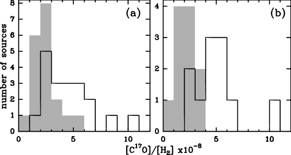
Figure 8: Distribution of C¹⁷O abundance. (a) The solid bars show the distribution of abundances for those sources with $\Delta v$(CS) $>$ 3 km s^-1 whilst the hollow bars represent those sources with $\Delta v$(CS) $<$ 3 km s^-1. (b) The solid bars show the distribution of abundances for the top 30% of the sample ($\Delta v$(CS) $\gg$ 3 km s^-1) while the hollow bars show the lower 30% of the sample ($\Delta v$(CS) $\ll$ 3 km s^-1).

6 Summary

We have presented spectra of 84 candidate HMPOs in the J $=2\rightarrow 1$ line of C¹⁷O and for a selection of these we have also observed C¹⁸O J $=2\rightarrow 1$ and C¹⁷O J $=3\rightarrow 2$. We have used the data to calculate the C¹⁷O column densities and for those sources for which models of dust emission exist we constructed models of the CO emission to check the validity of our assumptions regarding excitation temperature and dust temperature. We have found the following:

The ratio of C¹⁷O column density to H₂ derived from 850 $\mu$m dust emission has a significant scatter across our sample. The scatter between the most extreme sources is $\sim$14 and is consistent with the abundance of C¹⁷O differing on a source-by-source basis.

Our derivation of the H₂ column density assumed a constant value for $\kappa$ for all the sources, however there are no corrections to $\kappa$ which when applied globally to the sample to eliminate this scatter. Indeed the elimination of the scatter would require the sources lying at the extremes of the scatter to possess dust properties which are physical unlikely.

The method and assumptions used to calculate the C¹⁷O column densities were tested by modelling a subset of these sources with the radiative transfer code RATRAN. For all suitable models the best-fit abundance of C¹⁷O matched the data to within a factor of $\sim$2, supporting our assumptions and removing the possibility of the assumptions accounting for the range of abundances. We conclude that this scatter arises as a result of depletion present in a number of these sources. However the maximum degree of depletion we find does not exceed $\sim$7. This range of depletion suggests that outer regions of these sources have lifetimes during which they are cold and dense of about $2-4\times 10^{5}$ years.

We derive the mass-weighted temperature and find a correlation with C¹⁷O abundance, consistent with VVEB who from this correlation also infer the presence of depletion towards sources similar to those discussed here.

These sources have been studied by Beuther et al. (2002a) and a comparison of our C¹⁷O linewidths to their CS J $=3\rightarrow 2$ linewidths shows a division between those which have $\Delta v$(CS) $>$ 3 km s^-1 and those for which $\Delta v$(CS) $<$ 3 km s^-1. A statistical comparison of the C¹⁷O abundances of these two groups reveal a trend of the first group displaying significantly lower abundances than those in the second group with a statistical significance exceeding $\sim$98%.

We suggest that this range of C¹⁷O abundance and the implied degree of depletion between the sources may reflect a spread in evolutionary status amongst the sources. Higher angular resolution observations of dust emission, C¹⁷O and other species towards these objects will be important in confirming this suggestion. It is possible that high resolution observations will identify regions with higher degrees of depletion than can be measured with the relatively large telescope beam used for the observations presented here.

Depletion towards these objects shows that during the evolution of these cores the gas has remained cold and dense for long enough for the trace species to deplete. More detailed models of how trace molecules deplete in massive dense cores, combined with higher angular resolution observations, should be able to provide tighter constraints on the lifetime of these regions, including how long they exist before they form massive stars.

WFS	IRAS NAME	R.A.	Dec.	DATES OF OBSERVATIONS
		(J2000)	(J2000)	C18O (2$-$1)	C17O (2$-$1)	C17O (3$-$2)
WFS1	IRAS 05358+3543	05 39 10.8	$+$35 45 16		05/07/21	05/07/23
WFS3	IRAS 05490+2658	05 52 11.0	$+$27 00 34		05/07/21	05/07/23
WFS4	IRAS 05490+2658	05 52 12.1	$+$27 00 11		05/07/21	05/07/23
WFS6	IRAS 05553+1631	05 58 13.4	$+$16 32 00		05/07/21	05/07/23
WFS7	IRAS 18089-1732	18 11 45.2	$-$17 30 43			05/07/07
WFS8	IRAS 18089-1732	18 11 51.5	$-$17 31 34			05/07/07
WFS11	IRAS 18089-1732	18 11 57.0	$-$17 29 34			05/07/07
WFS12	IRAS 18090-1832	18 12 02.1	$-$18 31 58		05/08/03
WFS13	IRAS 18102-1800	18 13 11.7	$-$18 00 04		05/08/03
WFS14	IRAS 18151-1208	18 17 58.2	$-$12 07 28	04/05/13	04/05/13, 04/05/14
WFS15	IRAS 18159-1550	18 18 48.4	$-$15 49 00		05/08/03
WFS16	IRAS 18182-1433	18 21 08.9	$-$14 31 46	04/05/13	04/05/13
WFS17	IRAS 18223-1243	18 25 10.6	$-$12 42 27	04/05/13	04/05/14
WFS18	IRAS 18247-1147	18 27 31.4	$-$11 45 55		05/07/27, 05/08/03
WFS19	IRAS 18264-1152	18 29 14.3	$-$11 50 22		05/07/27, 05/08/03
WFS20	IRAS 18272-1217	18 30 02.2	$-$12 15 40	04/05/13	04/05/14
WFS21	IRAS 18272-1217	18 30 03.2	$-$12 15 11	04/05/13	04/05/14
WFS22	IRAS 18290-0924	18 31 43.4	$-$09 22 26	04/05/14	04/05/14	05/07/22
WFS23	IRAS 18290-0924	18 31 44.0	$-$09 22 17		05/08/03
WFS24	IRAS 18306-0835	18 33 17.3	$-$08 33 28		05/08/03
WFS25	IRAS 18306-0835	18 33 23.9	$-$08 33 33	04/05/13	04/05/13
WFS28	IRAS 18310-0825	18 33 47.9	$-$08 23 52		05/08/03
WFS29	IRAS 18337-0743	18 36 27.9	$-$07 40 25	04/05/14	04/05/14	05/07/22
WFS30	IRAS 18345-0641	18 37 16.8	$-$06 38 35	04/05/13	04/05/13
WFS33	IRAS 18348-0616	18 37 30.5	$-$06 14 13		05/07/27, 05/08/03
WFS34	IRAS 18372-0541	18 37 16.8	$-$06 38 35	04/05/14, 04/05/15	04/05/14
WFS35	IRAS 18385-0512	18 41 12.8	$-$05 08 58		05/08/03
WFS36	IRAS 18426-0204	18 45 12.1	$-$02 01 10	04/05/14, 04/05/15	04/05/14
WFS37	IRAS 18431-0312	18 45 45.5	$-$03 09 21		05/07/27, 05/08/03
WFS38	IRAS 18437-0216	18 46 21.8	$-$02 12 20		05/07/27, 05/08/03
WFS39	IRAS 18437-0216	18 46 22.4	$-$02 14 16	04/05/14, 04/05/15	04/05/14, 04/05/15	05/07/07
WFS41	IRAS 18440-0148	18 46 33.3	$-$01 44 52		05/08/03
WFS42	IRAS 18440-0148	18 46 36.5	$-$01 45 22		05/08/03
WFS51	IRAS 18460-0307	18 48 37.8	$-$03 03 48	04/05/14, 04/05/15	04/05/14, 04/05/15	05/07/07
WFS55	IRAS 18472-0022	18 49 52.4	$-$00 18 59		05/08/03
WFS57	IRAS 18488+0000	18 51 24.4	$+$00 04 39		05/07/26
WFS58	IRAS 18488+0000	18 51 25.5	$+$00 04 11		05/07/26
WFS59	IRAS 18521+0134	18 54 40.6	$+$01 38 05		05/08/03
WFS60	IRAS 18521+0134	18 54 44.4	$+$01 37 00		05/08/03
WFS61	IRAS 18530+0215	18 55 33.7	$+$02 19 09		05/08/03
WFS62	IRAS 18540+0220	18 56 36.6	$+$02 24 45		05/07/30
WFS63	IRAS 18540+0220	18 56 40.1	$+$02 25 30		05/07/30
WFS64	IRAS 18553+0414	18 57 53.5	$+$04 18 16		05/07/30
WFS66	IRAS 19012+0536	19 03 45.3	$+$05 40 43		05/08/03
WFS67	IRAS 19035+0641	19 06 01.5	$+$06 46 35		05/08/03
WFS68	IRAS 19074+0752	19 09 53.4	$+$07 57 12		05/07/29
WFS69	IRAS 19074+0752	19 09 53.9	$+$07 56 55		05/07/29
WFS70	IRAS 19175+1357	19 19 48.6	$+$14 02 26		05/07/27
WFS71	IRAS 19175+1357	19 19 48.8	$+$14 02 46		05/07/26
WFS72	IRAS 19217+1651	19 23 58.6	$+$16 57 38		05/07/27
WFS74	IRAS 19266+1745	19 28 55.5	$+$17 52 00		05/07/30
WFS75	IRAS 19282+1814	19 30 23.1	$+$18 20 22		05/07/30
WFS76	IRAS 19282+1814	19 30 29.7	$+$18 20 37		05/07/30
WFS77	IRAS 19403+2258	19 42 28.8	$+$23 05 03		05/07/28	05/07/07
WFS78	IRAS 19410+2336	19 43 10.6	$+$23 45 02	04/05/14	04/05/14	05/07/07
continued on next page

continued from previous page
WFS	IRAS NAME	R.A.	Dec.	DATES OF OBSERVATIONS
		(J2000)	(J2000)	C18O (2$-$1)	C17O (2$-$1)	C17O (3$-$2)
WFS79	IRAS 19410+2336	19 43 11.2	$+$23 44 06	04/05/14	04/05/14, 04/05/23	05/07/07
WFS80	IRAS 19411+2306	19 43 17.6	$+$23 13 57		05/07/28	05/07/07
WFS81	IRAS 19413+2332	19 43 26.3	$+$23 40 26		05/07/28	05/07/07
WFS82	IRAS 19413+2332	19 43 29.0	$+$23 40 19		05/07/29	05/07/07
WFS83	IRAS 19471+2641	19 49 10.1	$+$26 49 10		05/07/29	05/07/07
WFS84	IRAS 19471+2641	19 49 11.8	$+$26 49 38		05/07/29	05/07/07
WFS85	IRAS 20051+3435	20 07 04.5	$+$34 44 45		04/05/23
WFS86	IRAS 20081+2720	20 10 12.6	$+$27 29 13		05/07/26
WFS87	IRAS 20081+2720	20 10 13.3	$+$27 28 21		04/05/23
WFS88	IRAS 20081+2720	20 10 16.0	$+$27 28 12		04/05/23
WFS89	IRAS 20081+2720	20 10 18.7	$+$27 27 18		05/07/26
WFS90	IRAS 20126+4104	20 14 25.7	$+$41 13 30	04/05/14	04/05/13	05/07/21
WFS91	IRAS 20205+3948	20 22 20.0	$+$39 58 21	04/05/14	04/05/13	05/07/21
WFS92	IRAS 20205+3948	20 22 24.9	$+$39 57 55		05/07/26
WFS93	IRAS 20216+4107	20 23 23.9	$+$41 17 42		05/07/26
WFS94	IRAS 20293+3952	20 31 12.9	$+$40 03 21		05/07/27
WFS95	IRAS 20319+3958	20 33 49.4	$+$40 08 32		04/05/15
WFS96	IRAS 20332+4124	20 34 58.7	$+$41 34 46		04/05/15
WFS97	IRAS 20332+4124	20 35 01.1	$+$41 34 59		04/05/15
WFS98	IRAS 20343+4129	20 36 03.4	$+$41 39 44		05/07/27
WFS99	IRAS 20343+4129	20 36 06.3	$+$41 39 59	04/05/17	04/05/23
WFS100	IRAS 20343+4129	20 36 08.1	$+$41 39 58	04/05/17	04/05/23
WFS101	IRAS 22134+5834	22 15 08.9	$+$58 49 08		05/07/23
WFS102	IRAS 22551+6221	22 57 04.3	$+$62 37 44		05/07/23
WFS103	IRAS 22551+6221	22 57 07.4	$+$62 37 29		05/07/23
WFS104	IRAS 22551+6221	22 57 11.6	$+$62 36 46		05/07/23
WFS107	IRAS 22570+5912	22 59 05.0	$+$59 28 23	04/05/13	04/05/13	05/07/26
WFS108	IRAS 23033+5951	23 05 24.8	$+$60 08 14	04/05/13	04/05/13	05/07/26
WFS109	IRAS 23139+5939	23 16 09.8	$+$59 55 31	04/05/13	04/05/13	05/07/26
WFS110	IRAS 23151+5912	23 17 20.4	$+$59 28 51	04/05/14	04/05/22	05/07/26
WFS111	IRAS 23545+6508	23 57 02.1	$+$65 24 38	04/05/14	04/05/22	05/07/26
WFS112	IRAS 23545+6508	23 57 06.4	$+$65 24 49	04/05/14	04/05/22	05/07/26

Table 8: The telescope pointing coordinates are given along with the associated IRAS source found within the frame. The WFS labels refer to the submm peaks identified in Williams et al. (2004).

References

- Bensch et al. (2001) Bensch, F., Pak, I., Wouterloot, J. G. A., Klapper, G., & Winnewisser, G. 2001, ApJ, 562, 185
- Beuther et al. (2002a) Beuther, H., Schilke, P., Menten, K. M., Motte, F., Sridharan, T. K. & Wyrowski, F. 2002a, ApJ, 566, 945
- Beuther et al. (2002b) Beuther, H., Schilke, P., Sridharan, T. K., Menten, K. M., Walmsley, C. M. & Wyrowski, F. 2002b, A&A, 383, 892
- Caselli et al. (1999) Caselli, P., Walmsley, C. M., Tafalla, M. Dore, L. & Myers, P. C. 1999, ApJ, 523L, 165C
- Cesaroni et al. (2007) Cesaroni, R., Galli, D., Lodato, G., Walmsley, C. M. & Zhang, Q. 2007, Protostars and Planets V, B. Reipurth, D. Jewitt, and K. Keil (eds.), University of Arizona Press, Tucson, p197
- Flower (2001) Flower, D. R. 2001, JPhB, 34, 2731
- Flower et al. (2005) Flower, D. R., Pineau Des Forêts, G. & Walmsley, C. M. 2005, A&A, 436, 933
- Fontani et al. (2006) Fontani, F., Caselli, P., Crapsi, A., Cesaroni, R., Molinari, S., Testi, L. & Brand, J. 2006, A&A, 460, 709
- Frerking et al. (1982) Frerking, M. A., Langer, W. D & Wilson, R. W. 1982, ApJ, 262, 590
- Fuller et al. (2005) Fuller, G. A., Williams, S. J., & Sridharan, T. K. 2005, A&A, 442, 949
- Hatchell et al. (1998) Hatchell, J., Thompson, M. A., Millar, T. J., & MacDonald, G. H. 1998, A&A, 338, 713
- Hildebrand (1983) Hildebrand, R. H. QJRAS, 24, 267
- Hogerheijde & van der Tak (2000) Hogerheijde, M. R. & van der Tak, F. F. S. 2000, A&A, 362, 697
- Ivezić et al. (1999) Ivezić Ž., Nenkova M. & Elitzur M., 1999, User Manual for DUSTY, University of Kentucky Internal Report
- Kramer et al. (1999) Kramer, C., Alves, J., Lada, C. J., Lada, E. A., Sievers, A., Ungerechts, H., & Walmsley, C. M. 1999, A&A, 342, 257
- Kurtz et al. (2000) Kurtz, S., Cesaroni, R., Churchwell, E., Hofner, P. & Walmsley, C. M., 2000, Protostars & Planets IV, Univ. Arizona Press, Tucson, p299
- Ladd (2004) Ladd, E. F. 2004, ApJ, 610, 320
- Ladd et al. (1998) Ladd, E. F., Fuller, G. A., & Deane, J. R. 1998, ApJ, 495, 871
- Ossenkopf & Henning (1994) Ossenkopf, V., & Henning, Th., 1994, A&A, 291, 943
- Penzias (1981) Penzias, A. A. 1981, ApJ, 249, 518
- Redman et al. (2002) Redman, M. P., Rawlings, J. M. C., Nutter, D. J., Ward-Thompson, D. & Williams, D. A. 2002, MNRAS, 337L, 17
- Savva et al. (2003) Savva, D., Little, L. T., Phillips, R. R. & Gibb, A. G. 2003, MNRAS, 343, 259
- Schöier et al. (2005) Schöier, F. L, van der Tak, F. F. S., van Dishoeck, E. F. & Black, J. H. 2005, A&A, 432, 369
- Sheffer et al. (2002) Sheffer, Y., Lambert, D. L., & Federman, S. R. 2002, ApJ, 574, 171
- Shepherd (2005) Shepherd, D. 2005, IAU Symposium, 227, Massive Star Birth: A Crossroads of Astrophysics, Cesaroni, R., Felli, M., Churchwell, E., Walmsley, M. (eds) Cambridge: Cambridge University Press, p237
- Sridharan et al. (2002) Sridharan, T. K., Beuther, H., Schilke, P., Menten, K. M. & Wyrowski, F., 2002, ApJ, 566, 933 (SBSMW)
- Tafalla et al. (2002) Tafalla, M., Myers, P. C., Caselli, P., Walmsley, C. M. & Comito, C. 2002, ApJ, 569, 815
- Thomas & Fuller (2007) Thomas, H. S. & Fuller, G. A. 2007, ApJ, 659L, 165
- van der Tak et al. (2000) van der Tak, F. F. S., van Dishoeck, E. F., Evans, N. J. II & Blake, G. A. 2000, ApJ, 537, 283 (VVEB)
- van der Tak et al. (1999) van der Tak, F. F. S., van Dishoeck, E. F., Evans N. J., Bakker, E. J. & Blake, G. A. 1999, ApJ, 522, 911
- Viti & Williams (1999) Viti, S., & Williams, D. A. 1999, MNRAS, 305, 755
- Willacy et al. (1998) Willacy, K., Langer, W. D. & Velusamy, T. 1998, ApJ, 507L, 171
- Williams et al. (2004) Williams, S. J., Fuller, G. A. & Sridharan, T. K. 2004, A&A, 417, 115 (WFS04)
- Williams et al. (2005) Williams, S. J., Fuller, G. A. & Sridharan, T. K. 2005, A&A, 434, 257 (WFS05)
- Wouterloot et al. (2005) Wouterloot, J. G. A., Brand, J. & Henkel, C. 2005, A&A, 430, 549