Full Counting Statistics of Multiple Andreev Reflections in incoherent diffusive superconducting junctions
Abstract
We present a theory for the full distribution of current fluctuations in incoherent diffusive superconducting junctions, subjected to a voltage bias. This theory of full counting statistics of incoherent multiple Andreev reflections is valid for arbitrary applied voltage. We present a detailed discussion of the properties of the first four cumulants as well as the low and high voltage regimes of the full counting statistics. The work is an extension of the results of Pilgram and the author, Phys. Rev. Lett. 94, 086806 (2005).
1 Introduction
The mechanism for charge transport in voltage biased superconducting junctions is Multiple Andreev Reflections (MAR) KBT82 ; OTBK83 . Coherent MAR-theory CohMAR1 ; CohMAR2 ; CohMAR3 has provided a quantum mechanical picture for current transport in mesoscopic superconducting junctions. The predictions of the theory were found to be in impressive agreement with experimental results cohexp1 ; cohexp2 ; cohexp3 . This development, with the emphasis on the properties of atomic point contact junctions, was recently reviewed MARrew . Additional insight in coherent MAR transport, as e.g. the effective charge transferred, has been obtained by investigations of the current noise Blantrew , both theoretical CohTheoryNoise1 ; CohTheoryNoise2 ; CohTheoryNoise3 ; CohTheoryNoise4 and experimental CohExpNoise1 ; CohExpNoise2 ; CohExpNoise3 . Recently the theoretical interest has turned to the full distribution of current fluctuations Naz , the Full Counting Statistics (FCS) of coherent MAR-transport Johansson03 ; Cuevas03 ; Cuevas04 .
In several types of superconducting junctions, e.g. long diffusive superconducting-normal-superconducting (SNS) junctions, quasiparticles lose phase coherence when traversing the normal part of the junction and both the ac and dc Josephson currents are suppressed. This is the regime of incoherent MAR-transport. The properties of the current in the incoherent MAR-regime have been thoroughly studied, see e.g. Bez and references therein. In addition, in several works the current noise has been investigated, both theoretically LongTheoryNoise1 ; LongTheoryNoise2 ; LongTheoryNoise3 and experimentally LongDiff1 ; LongDiff2 ; LongDiff3 ; LongDiff4 . Recently experimental data on the third current cumulant in incoherent diffusive SNS junctions was presented by Reulet et al Reulet . Moreover, Pilgram and the author PilPRL presented a general theory for FCS of incoherent MAR. The theoretical result for a diffusive SNS junction showed qualitative similarities with the experimental data Reulet . The results in Ref. PilPRL were mainly derived with a stochastic path integral technique SPI1 ; SPI2 , however the extension of the FCS for diffusive SNS to arbitrary voltage bias was based on a more intuitive picture of incoherent MAR-transport. Appealing to this intuitive picture, in this work we first present a detailed derivation and then a thorough analysis of the FCS of incoherent MAR in diffusive SNS. Moreover, a formal derivation based on the stochastic path integral approach is presented in the appendix.
2 Model and theory
We consider a junction with a diffusive normal conductor connected to two superconducting terminals. The superconductors have an energy gap and a voltage is applied between the superconductors. The phase breaking length in the normal conductor is taken to be much shorter than the length of the conductor and the transport is consequently incoherent incohcond ; incohcond2 . We make the simplifying assumptions that the junction is perfectly voltage biased and that the scattering is completely elastic. The normal-superconducting(NS) interfaces are assumed to be transparent. Due to the diffusive nature of the transport, this gives that the effective Andreev reflection is perfect inside the superconducting gap (at quasiparticle energies ) and negligible outside the gap NagBut ; mycom1 . Throughout the paper we take the temperature to be well below the gap, , and consider only zero frequency transport properties.
In the paper we will appeal to a qualitative scattering picture of MAR CohMAR1 ; CohMAR2 ; Shum , a more formal derivation based on the approach of Ref. PilPRL ; SPI1 ; SPI2 is presented in the appendix. Within the scattering approach, the transport of quasiparticles in the junction can be described as MAR-transport in energy space Johansson : a quasiparticle below the gap injected from the superconductor into the normal conductor gain energy by successive Andreev reflections before escaping out into the superconductors at energies above the gap. This is illustrated to the left in fig. 1 for an applied voltage .
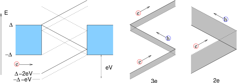
Due to the perfect effective Andreev reflection at the normal-superconducting interfaces, there are two possible processes by which a quasiparticle, injected from the left, can propagate from filled states below the gap to empty states above the gap.
for injection energies a quasiparticle traverses the gap three times (gaining an energy ) as electron hole electron, effectively transferring a charge from left to right.
for injection energies a quasiparticle traverses the gap twice (gaining an energy ) as electron hole, effectively transferring a charge from left to right.
The two transport processes are shown to the right in Fig. 1. Importantly, only these processes contribute to the net charge transport. We emphasize that in the scattering processes the net charge transferred across the junction is given by the electron charge multiplied by the net number of quasiparticle traversals or equivalently, the gained energy divided by the voltage . This holds independently on the injection energy and the type of quasiparticle injected Johansson03 . We also note that for quasiparticles injected from the right there are, due to the symmetry of the junction, two equivalent transport processes. Below, we for simplicity consider only the left injected quasiparticles and multiply all the derived transport properties with a factor of two.
2.1 Generalization to arbitrary voltage
The scenario presented above can be generalized to arbitrary applied voltage. We have that for a given voltage
| (1) |
there are two relevant transport processes for left injected quasiparticles.
quasiparticles injected at energies
| (2) |
traverse the junction times, transferring a charge from left to right (gaining an energy ).
quasiparticles injected at energies
| (3) |
traverse the junction times, transferring a charge from left to right (gaining an energy ). As emphasized above, no other processes transferring charge between occupied and unoccupied states are possible. Consequently, only these two processes (2) and (3) contribute to the net charge transport.
2.2 Effective diffusive transport
The MAR-transport in real space is diffusive. Since the transport is incoherent, neither the energy of the quasiparticle inside the normal conductor nor the electron or hole character of the quasiparticle is of importance for the transport properties. As a consequence, the process where a quasiparticle traverses the junction a net number of times, transferring a net charge , gives the same (zero frequency) transport statistics as a process where a quasiparticle with an effective charge is transported through normal diffusive conductors in series. The conductors in series have a conductance , with the conductance of the individual conductors doublecount . We point out that this effective model, illustrated in fig. 2, can be seen as a straightforward extension and combination of the noise models of refs. LongTheoryNoise2 ; LongTheoryNoise3 .
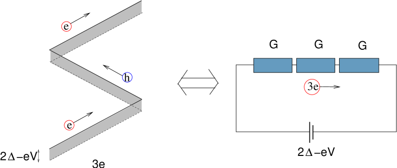
The “effective voltage” across the equivalent normal conductor is just the energy window available for the process (divided by ). Moreover, each of the two transport processes possible for a given voltage are independent. Consequently, the the total transport statistics is obtained by just summing up the contributions from the two processes. Importantly, since the FCS, or the transport statistics of diffusive conductors is known Lee , the above observation allows us to directly derive the FCS of the diffusive superconducting junction.
3 Cumulants of the current
Considering only positive voltages, we start with the average current. The current is the sum of the currents of two transport processes. For a voltage we have
| (4) | |||||
which is just Ohms law. Here, for clarity, we introduced the effective voltages for the two processes and . As is clear from Eq. (4), although the individual processes depend in a nontrivial way on the applied voltage via , the total current is just linear in voltage.
For the noise, the transport processes are associated with a certain noise power . For a diffusive conductor the noise power for conductors in series is , where the suppression factor comes from the diffusive nature of the transport BeenBut ; Nag2 . In addition, the noise is proportional to the effective charge squared. We can thus write the total noise
| (5) | |||||
which is the known result of Refs. LongTheoryNoise2 ; LongTheoryNoise3 . It is interesting to note that again the total noise shows no -dependence, it is a linear function of voltage, with a zero voltage offset. However, going to the third cumulant , the result does depend on , i.e. it displays a subharmonic gap structure in the form of kinks at voltages with . The expression for the third cumulant is given, along the same lines as for current and noise, by
| (6) |
In the same way we also get the fourth cumulant
| (7) |
The first four cumulants are plotted in fig. 3.
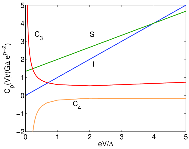
We see that, just as for a normal diffusive conductor, the first three cumulants are manifestly positive but the fourth cumulant is negative. In addition, while the first two cumulants are finite at low voltages, the third and fourth cumulants diverge for . Interestingly, in the experimental data Reulet the third cumulant shows a clear increase with decreasing voltage, down to a cut-off voltage. In this context we note that e.g. inelastic scattering, not accounted for in our model, will remove the low voltage divergences, similar to the situation for the noise CohTheoryNoise2 ; LongTheoryNoise2 ; LongTheoryNoise3 .
The subharmonic gap structure in the voltage dependence of the third and fourth cumulant is hardly visible in fig. 3. However turning to the differential cumulants, the derivatives of the cumulants with respect to the voltage, the subharmonic gap structure becomes apparent. The differential cumulants are shown in fig. 4.
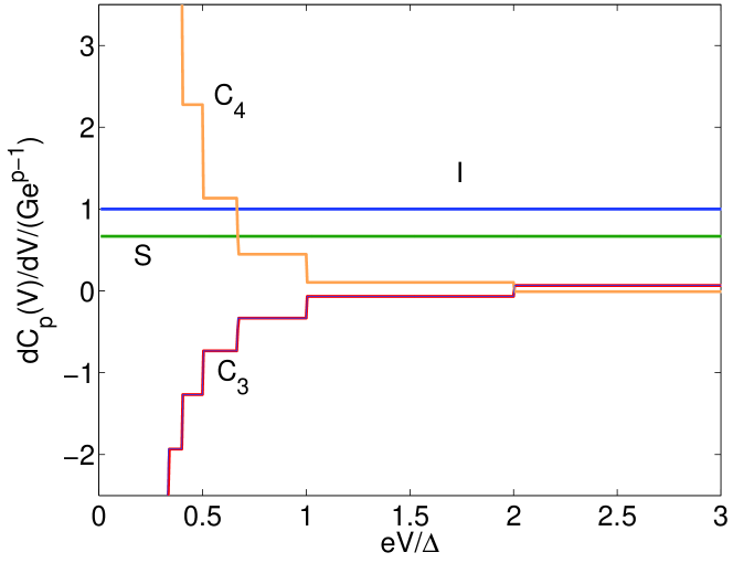
We note that the third and the fourth cumulants display a clear step structure. From Eqs. (6) and (7) we have
| (8) |
and
| (9) |
We point out that in contrast to the normalized cumulants in coherent single mode junctions in the tunneling regime CohTheoryNoise3 ; CohTheoryNoise4 ; Johansson03 ; Cuevas03 ; Cuevas04 , the height of the steps of the differential cumulants can not directly be related to an effective charge.
4 Full counting statistics
With the knowledge of the FCS of a normal diffusive conductor Lee , the scheme above can readily be extended to all higher cumulants. The cumulant generating function, from which the cumulants follow by successive derivatives with respect to the counting field , is then given by the sum of the generating functions for the two MAR-processes
| (10) | |||||
where is the measurement time. The current is , the noise , etc. We note that the distribution of transferred charge is given by a Fourier transform
| (11) |
Here we however do not further investigate the probability distribution, we instead turn to the low and high voltage limits of the cumulant generating function.
5 Voltage limits
5.1 Low voltage,
In the limit of low voltage, , we have and the cumulant generating function in Eq. (10) is given by
| (12) |
This is just the FCS for a normal diffusive conductor with an effective charge transferred. Importantly, as was found in Ref. PilPRL , this result (with different ) holds for an arbitrary incoherent superconducting junction. The origin of this universal behavior is that charge transport in incoherent superconducting junctions at low voltage bias can be described as diffusion in energy space. This energy diffusion was already noted for diffusive junctions, in the context of noise, in Refs. LongTheoryNoise2 ; LongTheoryNoise3 .
We note that the different cumulants behave as
| (13) |
This is different from the coherent (short) diffusive SNS-junctions investigated in Refs. Averin ; Johansson03 , where .
5.2 High voltage,
In the limit of high voltage, , giving in Eq. (1), the cumulant generating function in Eq. (10) is given by
| (14) |
The physical interpretation of this result follows directly from the model: the first term is due to single particle transport ( in the exponent) with an onset at while the second term is two-particle transport ( in the exponent). The “excess” fluctuations, the difference between the cumulant generating functions for the diffusive junction with the terminals in the superconducting and normal state respectively, is thus given by
| (15) |
We note that this result is independent on voltage. It gives the excess cumulants , , , etc.
6 Conclusions
In conclusion, we have investigated the full counting statistics of incoherent multiple Andreev reflections in diffusive SNS-junctions. An expression for the cumulant generating function has been derived. A careful analysis of the first four cumulants and the low and high voltage limits of the cumulant generating function has been presented. The results are valid under the assumptions of perfect voltage bias and the absence of inelastic scattering. To allow for a quantitative comparison with experiments for the full range of applied voltages, a theoretical model where these assumptions can be relaxed would be of great interest.
7 Acknowledgments
The author thanks Vitaly Shumeiko and Wolfgang Belzig for important comments on the manuscript. The work was supported by the Swedish VR.
8 Appendix
The cumulant generating function in Eq. (10) can be conveniently derived in a more formal way using the stochastic path integral approach SPI1 ; SPI2 applied to incoherent MAR PilPRL . We consider for simplicity a wire geometry, length , of the diffusive conductor (for a more general diffusive geometry, see Ref. SPI2 ). The starting point is to discretize the diffusive wire into nodes, contacted via quantum point contacts supporting transport modes with transparency . This discretization is shown in Fig. 5.
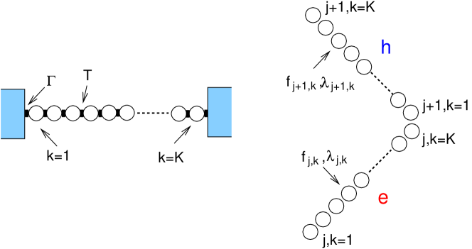
The transparency and the number of transport modes are chosen to give a conductance of the nodes in series equal to the conductance G of the wire.
The resulting node structure in energy space, along the MAR-ladder, is also shown in Fig. 5. Each node is characterized by a quasiparticle distribution function and a quasiparticle counting field , where is the number of the node and denotes the rung of the MAR-ladder. The :th rung goes between NS-interfaces at energies and where . We take for energies just below the gap , on the left side. The quasiparticles are thus electrons for rungs with odd and holes for even. Note also that is counted along the ladder, upwards in energy.
Following the scheme for FCS of incoherent MAR in Ref. PilPRL , we write the total generating function as a sum (energy integral) over the generating functions for different MAR-ladders, which contribute independently to the total generating function. This gives
| (16) |
where the generating function for a given MAR-ladder is a sum of the generating functions and along the ladder. Here
| (17) | |||||
is the generating function Levitov for the quantum point contact between nodes in the wire, with . The generating function describes the connection between nodes at the NS-interfaces Muzy ; Belzig . At energies inside the gap, , we have
| (18) | |||||
with the Andreev reflection probability and the normal reflection probability, where is the (normal) transparency of NS-interface. The counting field is taken equal to for odd and zero for even, i.e. the transferred charge is counted on the right side of the junction. It is important to note that counts electrical charge while counts quasiparticles.
Outside the gap, at , the Andreev reflection can effectively be neglected (as discussed above) and we can for simplicity consider a generating function for a perfect normal interface, i.e. a NS-interface with the superconductor taken in the normal state. This gives
| (19) | |||||
above the gap, and similarity below the gap. Here , with the quasipartice distribution function of the superconducting electrodes. For considered here, we have below the gap and above the gap.
To evaluate the generating functions for the ladders we first perform a transformation
| (20) |
[Under the stated conditions, only with are of interest]. This transformation removes the counting field from the generating functions of the NS-interfaces at energies inside the gap, in Eq. (18). In addition, the generating function for the NS-interface above the gap, Eq. (19) is modified as . This means that the counting field is transferred away from the interior of the ladder to the upper boundary.
Second, we the note that the structure of the generating functions for the quantum point contact between the nodes in the wire, Eq. (17), and for the NS-interface at energies inside the gap, Eq. (18), are formally identical when is transferred away (however with instead of ). The NS-interface thus effectively connects the end-nodes and of the two rungs and .
In addition, we emphasize that the boundary conditions (in the superconductors) for the distribution functions as well as the counting fields [after the transformation in Eq. (20)] are independent on the electron or hole character of the quasiparticles, they only depend on the energy . Consequently, the fact that distribution functions and counting fields describe electrons for odd and holes for even becomes irrelevant for the charge transfer and one thus only need to consider the position of the node in the MAR-ladder.
Taken together, the MAR ladder can thus be represented as a series of nodes, with equal to the number of rungs on the ladder, or equivalently the net number of absorbed energy quanta when traversing the junction. Note that since the resistance of the NS-interface is much smaller than the resistance of the diffusive wire, the details of the connection at the NS-interface ( instead of ) can be neglected. The only difference from a discretized normal diffusive wire of length is then the boundary condition for the counting field at the end of the wire, being instead of just for a normal wire.
Having performed this mapping to a discretized normal wire with renormalized boundary conditions we can continue with the standard procedure SPI2 to derive the total generating function in Eq. (16). We first denote the nodes with a single index running from to (dropping the rung index). In the limit the difference between distribution functions as well as counting fields of two neighboring nodes and is of the order and we can expand and . Inserting this expansion into the generating function in Eq. (17) we have to leading order in and
| (21) |
Taking the continuum limit and summing over all generating functions for different we get the generating function for a given energy as SPI2
| (22) |
where we have changed from summation over nodes to an integral over the dimensionless position along the wire, i.e and .
Second, this generating function is varied over all possible configurations of and . This results in a stochastic path integral formulation for the averaged generating function
| (23) |
Under the semiclassical conditions considered here, this path integral can be solved in the saddle point approximation. The saddle point equations are given by the functional derivatives
| (24) |
Solving these equations for and in terms of , inserting the solutions back into the generating function and performing the integration over then yields (see Ref. SPI2 for details)
| (25) |
describing the FCS of a diffusive wire with conductance and a renormalized charge . Finally, performing the integral over energy in Eq. (16), taking into account energy window for the two MAR-ladders, gives the generating function in Eq. (10). This concludes the formal derivation.
References
- (1) T. M. Klapwijk, G. E. Blonder, and M. Tinkham, Physica B+C 109-110, 1657 (1982).
- (2) M. Octavio, M. Tinkham, G. E. Blonder, and T. M. Klapwijk, Phys. Rev. B 27, 6739 (1983).
- (3) E.N. Bratus’, V.S. Shumeiko, and G. Wendin, Phys. Rev. Lett. 74, 2110 (1995).
- (4) D. Averin and A. Bardas, Phys. Rev. Lett. 75, 1831 (1995).
- (5) J.C. Cuevas, A. Martin-Rodero, and A. Levy-Yeyati, Phys. Rev. B 54, 7366 (1996).
- (6) N. van der Post, E. T. Peters, I. K. Yanson, and J. M. van Ruitenbeek, Phys. Rev. Lett. 73, 2611 (1994).
- (7) E. Scheer, P. Joyez, D. Esteve, C. Urbina, and M. H. Devoret E. Scheer, Phys. Rev. Lett.78, 3535 (1997).
- (8) E. Scheer, N. Agrait, J. C. Cuevas, A. Levy Yeyati, B. Ludoph, A. Mart n-Rodero, G. R. Bollinger, J. M. van Ruitenbeek, and C. Urbina, Nature 394, 154 (1998).
- (9) N. Agrait, A. Levy Yeyati, J. M. van Ruitenbeek, Phys. Rep. 377, 81 (2003).
- (10) Ya. M. Blanter and M. Büttiker, Phys. Rep. 336, 1 (2000).
- (11) J.P. Hessling, V. S. Shumeiko, Yu. M. Galperin and G. Wendin, Europhys. Lett. 34, 49 (1996).
- (12) D. Averin and H.T. Imam, Phys. Rev. Lett. 76, 3814 (1996)
- (13) J.C. Cuevas, A. Martin-Rodero, and A. Levy-Yeyati, Phys. Rev. Lett. 82, 4086 (1999).
- (14) Y. Naveh and D.V. Averin, Phys. Rev. Lett. 82, 4090 (1999).
- (15) P. Dieleman, H. G. Bukkems, T. M. Klapwijk,M. Schicke and K. H. Gundlach, Phys. Rev. Lett. 79, 3486 (1997).
- (16) R. Cron, M. F. Goffman, D. Esteve, and C. Urbina, Phys. Rev. Lett. 86, 4104 (2001).
- (17) F.E. Camino, V. V. Kuznetsov, E. E. Mendez, Th. Schp̈ers, V. A. Guzenko, and H. Hardtdegen, Phys. Rev. B 71, 020506(R) (2005).
- (18) See articles in Quantum Noise in Mesoscopic Physics, edited by Yu. V. Nazarov (Kluwer, Dordrecht, 2003).
- (19) G. Johansson, P. Samuelsson, Å. Ingerman, Phys. Rev. Lett. 91, 187002 (2003).
- (20) J. C. Cuevas and W. Belzig, Phys. Rev. Lett. 91, 187001 (2003).
- (21) J. C. Cuevas and W. Belzig, Phys. Rev. B 70, 214512 (2004).
- (22) E.V. Bezuglyi, E. N. Bratus, V. S. Shumeiko, G. Wendin, and H. Takayanagi, Phys. Rev. B 62, 14439 (2000).
- (23) E. V. Bezuglyi, E. N. Bratus, V. S. Shumeiko, and G. Wendin, Phys. Rev. Lett. 83, 2050 (1999).
- (24) K. E. Nagaev, Phys. Rev. Lett. 86, 3112 (2001).
- (25) E. V. Bezuglyi, E. N. Bratus, V. S. Shumeiko, and G. Wendin, Phys. Rev. B 63 100501 (2001).
- (26) X. Jehl, P. Payet-Burin, C. Baraduc, R. Calemczuk, and M. Sanquer, Phys. Rev. Lett. 83, 1660 (1999).
- (27) T. Hoss, C. Strunk, T. Nussbaumer, R. Huber, U. Staufer, and C. Schönenberger, Phys. Rev. B 62, 4079 (2000).
- (28) P. Roche, H. Perrin, D. C. Glattli, H. Takayanagi and T. Akazaki, Physica C 352, 73 (2001).
- (29) C. Hoffmann, F. Lefloch, and M. Sanquer, Euro. Phys. J B 29, 629 (2002).
- (30) B. Reulet, J. Senzier, D. Prober, L. Spietz, C. Wilson, and M. Shen, contribution to the summer school on “Nanoscopic Quantum Physics”, les Houches, 2004.
- (31) S. Pilgram and P. Samuelsson, Phys. Rev. Lett. 94, 086806 (2005).
- (32) S. Pilgram, A. N. Jordan, E. V. Sukhorukov, and M. Büttiker, Phys. Rev. Lett. 90, 206801 (2003).
- (33) A. N. Jordan, E. V. Sukhorukov, and S. Pilgram, J. Math. Phys. 45, 4386 (2004).
- (34) Incoherent MAR transport also occurs for an applied bias much larger than the Thouless energy of the normal conductor NagBut or for a time reversal symmetry breaking magnetic field in the normal conductor, as e.g. discussed in W. Belzig and P. Samuelsson, Europhys. Lett. 64, 253 (2003).
- (35) In the incoherent regime considered the proximity effect is completely suppressed. The effect of a finite proximity effect close to the NS-interfaces was investigated in Ref. Bez in the context of MAR.
- (36) K.E. Nagaev and M. Büttiker, Phys. Rev. B 63, 081301 (2001).
- (37) This can be understood as an analogy to the phenomena of reflectionless tunneling, B. J. van Wees, P. de Vries, P. Magn e, and T. M. Klapwijk, Phys. Rev. Lett 69, 510 (1992): E.g. an electron outside the gap, , incoming towards the NS-interface will either be transmitted (normal or Andreev) or reflected (normal or Andreev). If the particle is reflected it will, due to the diffusive transport in the wire, with large probability scatter back towards the NS-interface and ultimately be transmitted into the superconductor. Importantly, in this process, the net charge is transferred into the superconductor and the Andreev reflection can thus effectively be neglected. This scenario holds as long as the reistance of the NS-interface is much smaller than the resistance of the diffusive wire (see e.g. ref. Bez for a detailed discussion).
- (38) V.S. Shumeiko, E.N. Bratus and G. Wendin, Low. Temp. Phys. 23 181 (1997).
- (39) G. Johansson, K. N. Bratus, V. S. Shumeiko, and G. Wendin, Superlatt. and Microstr. 25, 905 (1999).
- (40) Note that in the scattering approach to superconducting systems Datta ; Shum electrons and holes, instead of spin up and spin down, are counted. As a consequence, the analogy between MAR-transport and normal transport gives the single spin transport statistics. A factor of two comes from counting also the right injected quasiparticles, as discussed in the text.
- (41) S. Datta, P. F. Bagwell and M.P. Anantram, Phys. Low-Dim. Struct. 3, 1 (1996).
- (42) H. Lee, L.S. Levitov, and A. Yu. Yakovets, Phys. Rev. B 51, 4079 (1996).
- (43) C.W.J. Beenakker, and M. Büttiker, Phys. Rev. B 46, 1889 (1992).
- (44) K.E. Nagaev, Phys. Lett. A 169, 103 (1992).
- (45) A. Bardas and D. V. Averin, Phys. Rev. B 56, R8518 (1997).
- (46) L.S. Levitov, H. Lee, and G.B. Lesovik, J. Math. Phys. (N.Y.) 37, 4845 (1996).
- (47) B.A. Muzykantskii and D.E. Khmelnitskii, Phys. Rev. B 50, 38982 (1994).
- (48) W. Belzig and Yu. V. Nazarov, Phys. Rev. Lett. 87, 197006 (2001).