Crossing paths in 2D Random Walks

Abstract

We investigate crossing path probabilities for two agents that move randomly in a bounded region of the plane or on a sphere (denoted $R$). At each discrete time-step the agents move, independently, fixed distances $d_{1}$ and $d_{2}$ at angles that are uniformly distributed in $(0,2\pi)$. If $R$ is large enough and the initial positions of the agents are uniformly distributed in $R$, then the probability of paths crossing at the first time-step is close to $2d_{1}d_{2}/(\pi A[R])$, where $A[R]$ is the area of $R$. Simulations suggest that the long-run rate at which paths cross is also close to $2d_{1}d_{2}/(\pi A[R])$ (despite marked departures from uniformity and independence conditions needed for such a conclusion).

1 Introduction

Random walks have been studied in abstract settings such as integer lattices $\mathbb{Z}^{d}$ or Riemannian manifolds ([4], [7], [10]). In applied settings there are many spatially explicit individual-based models (IBMs) in which the behavior of the system is determined by the meeting of randomly moving agents. The transmission of a pathogenic agent, the spread of a rumor, or the sharing of some property when randomly moving particles meet are examples that come to mind in biology, sociology, or physics ([3], [8], [6], [5], [2]). In many of these models the movement of agents is conceptualized as discrete transitions between square or hexagonal cells ([3]). However, such a stylized representation of individual movements may not always be entirely realistic.

Although IBMs are powerful tools for the description of complex systems, they suffer from a shortage of analytical results. For example, if a susceptible and an infective agent move randomly in some bounded space, what is the probability of them meeting, and hence of the transmission of the infection? What is the average time until the meeting takes place?

In the present paper we begin to answer these questions by considering a random walk in a bounded region of the plane or on the sphere, which we denote by $R$. The model evolves in discrete time. At each time-step an agent leaves its current position at a uniformly distributed angle in the $(0,2\pi)$ interval. On the plane the agent moves a fixed distance $d$ in a straight line. On a sphere the agent moves a fixed distance $d$ on a geodesic.

Here we will consider two such agents who move different distances $d_{1}$ and $d_{2}$ at each time-step. We assume that the agents’ initial positions are uniformly distributed in $R$. The paper’s central results concern the probability that the paths of the two agents cross during the first time-step. If $R$ is either a sufficiently large bounded region of the plane or a sphere, this ”first-step” probability of intersection is close to $2d_{1}d_{2}/(\pi A[R])$ where $A[R]$ is the area of $R$.

In applied settings we are often interested in the long-run average rate at which the paths cross. In order to extend results on the ”first-step” probability of intersection and apply the law of large numbers we would need the following assumptions:

• The positions of the two agents are uniformly distributed at every time step (which is the case on the sphere but not on the plane because of reflection problems at the boundary of $R$),

• The crossing-path events are independent over time (which is the case in neither setting because of the strong spatial dependence at consecutive time-steps).

Numerous simulations have shown that despite marked departures from these assumptions the long-run rate at which the paths cross is also close to $2d_{1}d_{2}/(\pi A[R])$.

Section 2 contains the results both for the plane and the sphere. Section 3 is devoted to the numerical simulations. Extensions are discussed in Section 4. Three technical appendices can be found in Section 5.

Fig. 1: Example of two trajectories ${V_{1}(k)}$ and ${V_{2}(k)}$ with paths that crossed synchronously at $m_{1}$ for $k=2$. (We are not interested in the asynchronous crossing at $m_{2}$ which took place at different times for the two agents).

2 Model

2.1 Geometric description in the plane and on the sphere

A bounded region of the plane is the most natural setting for agents moving in a 2D environment. However we then need to specify how agents are reflected when they hit the boundary of the region. There is no such problem on a sphere. In what follows $R$ is either a bounded region of the plane or a sphere.

The initial positions ${V_{1}(0)}$ and ${V_{2}(0)}$ of the two agents are assumed uniformly distributed in $R$. At each time-step the two agents move distances $d_{1}$ and $d_{2}$ (which are fixed positive parameters) in a straight line (or along a geodesic on a sphere). They depart at random angles $\alpha_{1}$ and $\alpha_{2}$ that are uniformly and independently distributed over $(0,2\pi)$. The endpoints after the $k-th$ time-step are $V_{1}(k)$ and $V_{2}(k)$ (Figure 1).

The definition of a meeting in such a model is tricky because the probability of the two agents being in exactly the same position at any given period is 0. There are however different ways of approximating such a meeting.

One could say that the agents meet if the distance between two points ${V_{1}(k)}$ and ${V_{2}(k)}$ is less than some $\epsilon$. In such a definition results would depend on $\epsilon$, which is undesirable. For this reason we choose to define a meeting during the $k-th$ time-step when paths cross between $k$ and $k+1$. This means that the segments (or the ”geodesic arcs”) $V_{1}(k)V_{1}(k+1)$ and $V_{2}(k)V_{2}(k+1)$ intersect. We recognize that ${V_{1}(k)}$ and ${V_{2}(k)}$ can then be close without the paths crossing, but at least the definition does not depend on some arbitrary $\epsilon$.

The point $m_{1}$ in Figure 1 is an example of such a synchronous crossing of paths. Of course the agents are not at $m_{1}$ at the same time. In the figure the paths cross asynchronously at $m_{2}$.

Much will depend on whether ${V_{1}(k)}$ and ${V_{2}(k)}$ are uniformly distributed on $R$ for every $k$. This will be the case if $R$ is a sphere because ${V_{1}(0)}$ and ${V_{2}(0)}$ are themselves uniformly distributed. If on the other hand $R$ is a bounded region of the plane, then the uniformity in the distributions of ${V_{1}(k)}$ and ${V_{2}(k)}$ is compromised for $k>0$ by the vexing problem of the behavior of the agents when they hit the boundary of $R$.

For this reason we focus on the probability of paths crossing at the first time-step only. We simplify notations by letting $V_{1}\overset{def.}{=}(x_{1},y_{1})$ and $V_{2}\overset{def.}{=}(x_{2},y_{2})$ be the initial positions of the two agents. The corresponding endpoints are denoted $W_{1}$ and $W_{2}$.

We next proceed with calculations when $R$ is a bounded region of the plane.

2.2 Crossing-path probability in a bounded region of the plane

In the plane the endpoints $W_{1}$ and $W_{2}$ are

$$W_{1}\overset{def.}{=}V_{1}+d_{1}(cos(\alpha_{1}),sin(\alpha_{1}))$$ (1)

$$W_{2}\overset{def.}{=}V_{2}+d_{2}(cos(\alpha_{2}),sin(\alpha_{2}))$$ (2)

where $\alpha_{1}$ and $\alpha_{2}$ are polar angles that are uniformly distributed in $(0,2\pi)$.

We will finesse the reflection problem at the boundary of $R$ by considering the possibility of intersection on the basis of Eqs. (1) - (2) even if $W_{1}$ or $W_{2}$ is outside $R$. In such a case we examine first whether the intersection has occurred. We then move, in some unspecified manner, the wayward point(s) back inside $R$.

We now define the feasible domain $FD(V_{1},\alpha_{1})$ as the set of points $V$ that are within $d_{2}$ of the segment $V_{1}W_{1}$:

$$FD(V_{1},\alpha_{1})\overset{def.}{=}\left\{V=(x,y)\mbox{ such that }d(V,(V_{1}W_{1}))\leq d_{2}\right\}$$ (3)

where $d(V,(V_{1}W_{1}))$ is the distance between a point $V$ and the segment $V_{1}W_{1}$.

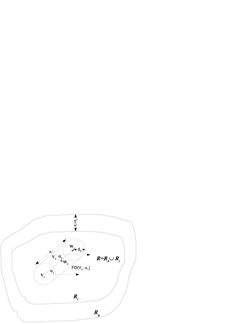
Fig. 2: Example of two intersecting segments $V_{1}W_{1}$ and $V_{2}W_{2}$ with feasible domain $FD(V_{1},\alpha_{1})$. Inner and border regions $R_{i}$ and $R_{b}$ are at distances to the outside world that are larger than and less than the sum $d_{1}+d_{2}$. (The distance $d_{1}+d_{2}$ between the two boundaries is not to scale).

The point $V_{2}$ must be in $FD(V_{1},\alpha_{1})$ in order for the segments $V_{1}W_{1}$ and $V_{2}W_{2}$ to intersect - although the condition is not sufficient. Figure 2 depicts a segment $V_{1}W_{1}$ and the corresponding feasible domain $FD(V_{1},\alpha_{1})$. This domain is bounded by dotted lines (a rectangle with sides $d_{1}$ and $2d_{2}$ with a half circle of radius $d_{2}$ at each end of the rectangle). In the figure a point $V_{2}$ is in the feasible domain and the two segments $V_{1}W_{1}$ and $V_{2}W_{2}$ intersect. Whether there is an intersection depends on the angle $\alpha_{2}$.

The region $R$ is partitioned into an inner region $R_{i}$ and a border region $R_{b}$ characterized by a distance to the outside world that is either larger (for $R_{i}$) or smaller (for $R_{b}$) than $d_{1}+d_{2}$. (The point is that $FD(V_{1},\alpha_{1})$ is entirely in $R$ if $V_{1}\in R_{i}$). We define$A[S]$ as the area of a bounded subset $S$ of $\mathbb{R}^{2}$.

With $V_{1}=(x_{1},y_{1})$ and $V_{2}=(x_{2},y_{2})$ uniformly and independently distributed on $R$, we will now calculate the probability that $V_{1}W_{1}$ and $V_{2}W_{2}$ intersect. This first-step probability of intersection depends only on $d_{1},d_{2}$ and $R$, and is noted $P_{p}(d_{1},d_{2},R)$. (The subscript $p$ indicates a probability in the plane).

We first need the probability $G_{p}(x_{1},y_{1},\alpha_{1})$ of the intersection conditionally on $V_{1}=(x_{1},y_{1})$ and $\alpha_{1}$; $G_{p}(x_{1},y_{1},\alpha_{1})$ is the probability (denoted by $p_{1}$ below) that $V_{2}$ falls in $FD((x_{1},y_{1}),\alpha_{1})\bigcap R$ multiplied by the probability (denoted by $p_{2}$ below) of the segments intersecting conditionally on $V_{2}$ falling in $FD((x_{1},y_{1}),\alpha_{1})\bigcap R$. (In the $FD$ function we have replaced $V_{1}$ by its coordinates $(x_{1},y_{1})$).

Given the uniformity assumption on $V_{2}$, the probability $p_{1}$ is then

$$p_{1}=\dfrac{A[FD((x_{1},y_{1}),\alpha_{1})\bigcap R]}{A[R]}.$$ (4)

In order to calculate $p_{2}$ we need to define the probability $f_{p}(x_{1},y_{1},\alpha_{1},x_{2},y_{2})$ that $V_{2}W_{2}$ intersects $V_{1}W_{1}$, conditionally on $V_{1}=(x_{1},y_{1}),V_{2}=(x_{2},y_{2})$ and the angle $\alpha_{1}$. (This probability, derived in Appendix A, is obtained by calculating the magnitude of the angle $\beta$ within which $\alpha_{2}$ must fall for the intersection to occur, and then dividing by $2\pi$). The conditional probability $p_{2}$ of the intersection is then

$$p_{2}=\dfrac{\iint_{(x_{2},y_{2})\in FD((x_{1},y_{1}),\alpha_{1})\bigcap R}f_{p}(x_{1},y_{1},\alpha_{1},x_{2},y_{2})dx_{2}dy_{2}}{A[FD((x_{1},y_{1}),\alpha_{1})\bigcap R]}.$$ (5)

The probability $G_{p}(x_{1},y_{1},\alpha_{1})$ is now the product $p_{1}p_{2}$ which simplifies to

$$G_{p}(x_{1},y_{1},\alpha_{1})=\dfrac{\iint_{(x_{2},y_{2})\in FD((x_{1},y_{1}),\alpha_{1})\bigcap R}f_{p}(x_{1},y_{1},\alpha_{1},x_{2},y_{2})dx_{2}dy_{2}}{A[R]}.$$ (6)

When $V_{1}=(x_{1},y_{1})$ is in $R_{i}$ (i.e. the feasible domain is entirely in $R$) then the double integral on the right-hand side of Eq. (6) is independent of $V_{1}$ and is noted $I_{p}(d_{1},d_{2})$, i.e.

$$I_{p}(d_{1},d_{2})\overset{def.}{=}\iint_{(x_{2},y_{2})\in FD((x_{1},y_{1}),\alpha_{1})}f_{p}(x_{1},y_{1},\alpha_{1},x_{2},y_{2})dx_{2}dy_{2}.$$ (7)

The quantity $I_{p}(d_{1},d_{2})$ is an upper bound for the double integral in Eq. (6) when $V_{1}=(x_{1},y_{1})$ is in the border region $R_{b}$ (because the integration is then over an area smaller than the feasible domain $FD(x_{1},y_{1})$).

We now have the following result on $I_{p}(d_{1},d_{2})$, $G_{p}(x_{1},y_{1},\alpha_{1})$, and $P_{p}(d_{1},d_{2},R)$.

Proposition 1.

We have

$$I_{p}(d_{1},d_{2})=2d_{1}d_{2}/\pi$$ (8)

and when $V_{1}=(x_{1},y_{1})$ is in $R_{i}$,

$$G_{p}(x_{1},y_{1},\alpha_{1})=\dfrac{2d_{1}d_{2}}{\pi A[R]}.$$ (9)

When $V_{1}=(x_{1},y_{1})$ is in $R_{b}$ then

$$G_{p}(x_{1},y_{1},\alpha_{1})\leq\dfrac{2d_{1}d_{2}}{\pi A[R]}.$$ (10)

The first-step probability of intersection $P_{p}(d_{1},d_{2},R)$ satisfies

$$p_{\ell o}\overset{def.}{=}\dfrac{2d_{1}d_{2}A[R_{i}]}{\pi A[R]^{2}}\leq P_{p}(d_{1},d_{2},R)\leq p_{hi}\overset{def.}{=}\dfrac{2d_{1}d_{2}}{\pi A[R]}$$ (11)

which leads to the mid-point approximation

$$P_{p}(d_{1},d_{2},R)\approxeq p^{*}\overset{def.}{=}d_{1}d_{2}\dfrac{A[R_{i}]+A[R]}{\pi A[R]^{2}}.$$ (12)

The absolute value of the maximum percentage error (AVMPE) made with the approximation of (12) is

$$AVMPE=100\dfrac{A[R]-A[R_{i}]}{A[R]+A[R_{i}]}.$$ (13)

Proof.

See Appendix A. ∎

Remark. The approximation of Eq. (12) is of interest and the error of Eq. (13) is small only if $A[R]$ is large enough in the sense that $A[R_{i}]$ is relatively close to $A[R]$. This means there is a large subset of $R$ within which the feasible domain $FD(V_{1},\alpha_{1})$ is entirely in $R$. Suppose for example that $R$ is a circle of radius $r>d_{1}+d_{2}$, then

$$AVMPE=100\dfrac{1-\left(1-\frac{d_{1}+d_{2}}{r}\right)^{2}}{1+\left(1-\frac{d_{1}+d_{2}}{r}\right)^{2}}$$ (14)

which is approximately $100(d_{1}+d_{2})/r$ when $d_{1}+d_{2}$ is much smaller than $r$. Therefore if $d_{1}+d_{2}$ is one percent of the radius then the maximum error made with the estimate of Eq. (12) is also approximately one percent.

We next turn our attention to the situation in which $R$ is a sphere.

2.3 Crossing-path probability on a sphere

When the domain $R$ is a sphere of radius $\rho$ we use the spherical system of coordinates where a point $V$ is defined by the triplet $(\rho,\theta,\phi)$ of radial, azimuthal, and zenithal coordinates.

Given initial points $V_{k}\overset{def.}{=}(\rho,\theta_{k},\phi_{k}),(k=1,2)$ each endpoint $W_{k}$ is on the circle at a geodesic distance $d_{k}$ from $V_{k}$. The position of $W_{k}$ on the circle is determined by an angle $\alpha_{k}$ uniformly distributed in $(0,2\pi)$. See Appendix B for the exact derivation of the endpoints $W_{k}$.

We let $P_{s}(d_{1},d_{2},R)$ be the probability that the arcs $V_{1}W_{1}$ and $V_{2}W_{2}$ intersect. Because the initial points $V_{k}$ are uniformly distributed, the endpoints will also be uniformly distributed on the sphere. Therefore $P_{s}(d_{1},d_{2},R)$ is the probability of paths crossing at every time-step.

In order to calculate $P_{s}(d_{1},d_{2},R)$ we proceed as before except that there is no border area and the double integrals are calculated in spherical coordinates. The feasible domain is denoted $FD(\theta_{1},\phi_{1})$ and is defined with geodesic distances. The differential area element is now $\rho^{2}sin(\phi)d\theta d\phi$.

We let $f_{s}(\theta_{1},\phi_{1},\alpha_{1},\theta_{2},\phi_{2})$ be the probability of intersection conditionally on the arc $V_{1}W_{1}$ (defined by $\theta_{1},\phi_{1}$ and $\alpha_{1}$) and on $V_{2}$ (defined by $\theta_{2}$ and $\phi_{2}$). We also define the double integral

$$I_{s}(d_{1},d_{2},\rho)\overset{def.}{=}\iint_{(\theta_{2},\phi_{2})\in FD((\theta_{1},\phi_{1}),\alpha_{1})}f_{s}(\theta_{1},\phi_{1},\alpha_{1},\theta_{2},\phi_{2})\rho^{2}sin(\phi_{2})d\theta_{2}d\phi_{2}.$$ (15)

The probability of the intersection conditionally on $V_{1}=(\rho,\theta_{1},\phi_{1})$ and $\alpha_{1}$ is independent of $\rho,\theta_{1},\phi_{1}$ and is denoted $G_{s}(d_{1},d_{2},\rho)$. We then have

$$G_{s}(d_{1},d_{2},\rho)=\dfrac{I_{s}(d_{1},d_{2},\rho)}{A[R]}$$ (16)

where the area $A[R]$ of the sphere appearing in the denominator is now $4\pi\rho^{2}$.

The probability of paths crossing at each time-step is then

$$P_{s}(d_{1},d_{2},R)=\dfrac{\iiint_{(\theta_{1},\phi_{1})\in R,\alpha_{1}\in(0,2\pi)}G_{s}(\theta_{1},\phi_{1},\alpha_{1})\rho^{2}sin(\phi_{1})d\theta_{1}d\phi_{1}d\alpha_{1}}{2\pi A[R]}$$

$$=\dfrac{I_{s}(d_{1},d_{2},\rho)}{A[R]}=\dfrac{I_{s}(d_{1},d_{2},\rho)}{4\pi\rho^{2}}.$$ (17)

When $\rho\rightarrow\infty$ the integral $I_{s}(d_{1},d_{2},\rho)$ on the sphere approaches the corresponding integral $I_{p}(d_{1},d_{2})=2d_{1}d_{2}/\pi$ on the plane (Eq. (8)).

In the next proposition we show numerically that $I_{s}(d_{1},d_{2},\rho)$ is extremely close to $2d_{1}d_{2}/\pi$ even when $\rho$ is not particularly large compared to $d_{1}$ and $d_{2}$. We will just assume that

$$\dfrac{d_{2}}{\rho}<\dfrac{\pi}{2},\dfrac{d_{1}}{2\rho}+\dfrac{d_{2}}{\rho}<\pi$$ (18)

which insures that the feasible domain does not ”wrap around” the sphere.

Proposition 2.

With (18) we have

$$I_{s}(d_{1},d_{2},\rho)\approxeq 2d_{1}d_{2}/\pi$$ (19)

and the probability of paths crossing at each time-step is

$$P_{s}(d_{1},d_{2},R)\approxeq\dfrac{2d_{1}d_{2}}{\pi A[R]}=\dfrac{d_{1}d_{2}}{2\pi^{2}\rho^{2}}.$$ (20)

The differences between both sides of (19) and (20) are so small that they are within the margins of error when calculating $I_{s}(d_{1},d_{2},\rho)$ (and $P_{s}(d_{1},d_{2},R)$) numerically.

Proof.

See Appendix C. ∎

The next section is devoted to simulations aimed at assessing the quality of the approximations derived above.

3 Simulations

We consider a region $R$ that is a circle of radius $r=10$. At each time-step the two agents move distances $d_{1}=1$ and $d_{2}=0.7$ respectively. If an agent moves outside the circle we first check whether paths have crossed. We then move the wayward agent to a point diametrically opposed to its current position, at a distance inside the circle equal to the distance between the circle and the current position. This algorithm could be considered a 2D version of the wrapping around that takes place on a sphere. The goal is to try to keep the distribution of the agents as uniform as possible. We need this in order for the crossing-path probability to remain as close as possible to the ”first-step” probability derived under the assumption that initial positions are uniformly distributed.

The bounds of (11) and the approximation of (12) are now used to calculate the low, high and mid-point approximations $p_{\ell o},p_{hi},p^{*}$ for the first-step probability of intersection $P_{s}(d_{1},d_{2},\rho)$:

$$p_{\ell o}=\dfrac{2d_{1}d_{2}A[R_{i}]}{\pi A[R]^{2}}=0.0009772,\vskip 12.0pt plus 4.0pt minus 4.0ptp_{hi}=\dfrac{2d_{1}d_{2}}{\pi A[R]}=0.001418,$$ (21)

$$p^{*}=d_{1}d_{2}\dfrac{A[R_{i}]+A[R_{b}]}{\pi A[R]^{2}}=0.001198$$ (22)

which translate into a maximum error $AVMPE$ on $p^{*}$ of 18.42% (Eq. (14)). This error is relatively large because the sum $d_{1}+d_{2}$ is 1.7, which is not particularly small compared to the radius 10 of the circle.

We let $F(k)$ be the random variable equal to the average crossing path frequency over the first $k$ time-steps. If the probability of paths crossing at every time-step were $p_{\ell o}$ (or $p_{hi}$) and if paths crossing were independent events (which they are not) then the Central Limit Theorem would insure that for large $k$ the corresponding ”hypothetical frequency” $F_{h}(k)$ would be approximately normally distributed with mean $p_{\ell o}$ (or $p_{hi}$) and standard deviation $\sqrt{p_{\ell o}(1-p_{\ell o})/k}$ (or $\sqrt{p_{hi}(1-p_{hi})/k}$).

Figure 3 depicts a simulated trajectory of the frequency $F(k)$. We also plotted the hypothetical low and high intervals within which each $F_{h}(k)$ would fall with probability $0.95$. These bands shed light on the expected fluctuations of the frequency, in the case of independent events taking place with probability $p_{\ell o}$ (or $p_{hi}$).

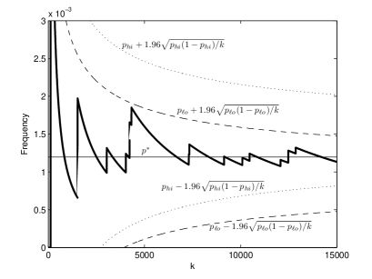
Fig. 3: Average crossing-path frequency $F(k)$ (over the first $k$ time-steps) for two random walks in a circle of radius $r=10$ with $d_{1}=1$ and $d_{2}=0.7$ (15,000 time-steps). At each time-step the intervals within which the ”hypothetical frequency” $F_{h}(k)$ falls with probability $0.95$ are given for the low and high approximations $p_{\ell o}$ and $p_{hi}$ of $P(d_{1},d_{2},\rho)$. The mid-point approximation $p^{*}$ is also plotted.

This and other simulations suggest that $p^{*}$ gives at least an idea of the (long-run) crossing-path probability.

There is less uncertainty on the sphere as we have shown that the one-step probability of intersection $P_{s}(d_{1},d_{2},R)$ is extremely close to $d_{1}d_{2}/(2\pi^{2}\rho^{2})$. Simulations performed on the sphere (not shown) yield long-run crossing-path rates that are close to $d_{1}d_{2}/(2\pi^{2}\rho^{2})$ even though the law of large numbers cannot be invoked because of spatial dependence over time.

4 Discussion

The expression of Eq. (12) for the crossing-path probability in the plane can be relatively crude. However it has the merit of simplicity and it improves if the area of the region $R$ increases.

On the sphere the crossing-path probability can be approximated very closely by the simple expression $d_{1}d_{2}/(2\pi^{2}\rho^{2})$. We derived this expression on the basis of an analytical result for the plane (Appendix A), expecting it to be a good approximation only for a sphere of infinitely large radius. It is of some interest to note that because of the complexity of the multiple integrals in spherical coordinates we saw now way of obtaining this approximation from the calculations performed directly on the sphere (Appendix C).

Because of marked departures from required assumptions the law of large numbers could be applied neither in the plane nor on the sphere. Despite that, the long-run average crossing-path probabilities appear to be close to the first-step probabilities. This suggests that a weaker version of the law of large numbers may be applicable. For example results on ”weakly dependent” random variables (i.e. variables that are ”m” (or ”$\varphi$”)-dependent ([9])) may provide more insights into the long-run behavior of the system.

We note some obvious and some less obvious extensions that can be of use to population biologists (and perhaps others):

• If the crossing of paths takes place between an infected and a susceptible agent, then the transmission of the infection may occur with only a probability $\tau$. In such a case the crossing-path probabilities found here need simply be multiplied by $\tau$ in order to obtain the probability of transmission at each time-step.

• An important extension would have $I$ such infectives and $S$ such susceptibles. Epidemiologists would be keenly interested in analytical results on the rate at which the infection would then spread.

• The assumption that an agent moves at an angle that is uniformly distributed in (0,2$\pi$) may not be realistic. For example animals may move only within a limited angle in the continuation of the previous direction. Preliminary investigations suggest that the results obtained here may still be applicable.

The results given in this paper are merely starting points for more in-depth theoretical investigations. They also provide practitioners with some answers concerning the dynamics of a process that depends on randomly moving agents meeting in a spatially explicit environment.

5 Appendices

5.1 Appendix A: Proof of Proposition 1

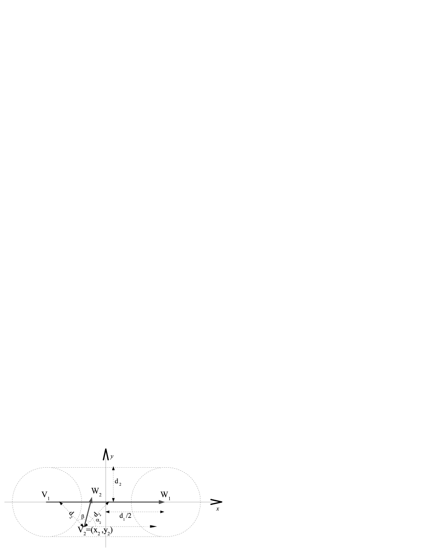
Fig. 4: Intersecting segments $V_{1}W_{1}$ and $V_{2}W_{2}$ in coordinate system in which $V_{1}W_{1}$ lies on the $x$-axis and the origin is at the middle of $V_{1}W_{1}$.

The double integral $I_{p}(d_{1},d_{2})$ in Eq. (6) is calculated in the orthonormal coordinate system $(x,y)$ for which the segment $V_{1}W_{1}$ lies on the $x$-axis and the origin is at the middle of the segment (Figure 4).

In the new coordinate system, the probability $f_{p}(x_{1},y_{1},\alpha_{1},x_{2},y_{2})$ that $V_{1}W_{1}$ and $V_{2}W_{2}$ intersect depends only on the components $(x_{2},y_{2})$ of $V_{2}$. If this probability is denoted $F_{p}(x_{2},y_{2})$, then $I_{p}(d_{1},d_{2})$ is

$$I_{p}(d_{1},d_{2})=\int_{y=-d_{2}}^{y=d_{2}}\int_{x=-d_{1}/2-\sqrt{d_{2}^{2}-y^{2}}}^{x=d_{1}/2+\sqrt{d_{2}^{2}-y^{2}}}F_{p}(x,y)dxdy.$$ (23)

The probability $F_{p}(x_{2},y_{2})$ is obtained by calculating the magnitude of the angle $\beta$ within which $V_{2}W_{2}$ (defined by the angle $\alpha_{2}$) must fall and then dividing by $2\pi$ (see Figure 4). In the Figure the point $V_{2}$ is in neither circle and the angle $\beta$ is the vertex angle in the isosceles triangle with apex $V_{2}$ and two sides of length $d_{2}$. Therefore, when $V_{2}$ is in neither circle the probability $F_{p}(x_{2},y_{2})$ of an intersection is given by the function

$$F_{p,1}(x_{2},y_{2})\overset{def.}{=}\dfrac{2\arccos\left(\dfrac{|y_{2}|}{d_{2}}\right)}{2\pi}.$$ (24)

Similar geometric considerations show that if the two circles overlap (i.e. $d_{1}/2<d_{2}$) then for a point $(x_{2},y_{2})$ in the intersection of the two circles, the probability of intersection $F(x_{2},y_{2})$ is given by the function

$$F_{p,2}(x_{2},y_{2})\overset{def.}{=}\dfrac{\arctan\left(\dfrac{x_{2}+d_{1}/2}{|y_{2}|}\right)-\arctan\left(\dfrac{x_{2}-d_{1}/2}{|y_{2}|}\right)}{2\pi}.$$ (25)

Finally, if $(x_{2},y_{2})$ is in only one of the circles, then one of the vertices of the triangle with apex $V_{2}$ will be the center $V_{1}$ or $W_{1}$ of that circle. The probability of intersection $F(x_{2},y_{2})$ is then

$$F_{p,3}(x_{2},y_{2})\overset{def.}{=}\dfrac{\arccos\left(\dfrac{|y_{2}|}{d_{2}}\right)-\arctan\left(\dfrac{x_{2}-d_{1}/2}{|y_{2}|}\right)}{2\pi}.$$ (26)

Long but elementary calculations show that the innermost integral in (23), considered a function $H(y)$ of $y$, is now equal to

$$H(y)\overset{def.}{=}\int_{x=-d_{1}/2-\sqrt{d_{2}^{2}-y^{2}}}^{x=d_{1}/2+\sqrt{d_{2}^{2}-y^{2}}}F_{p}(x,y)dx=\dfrac{d_{1}\times\arccos\left(\dfrac{|y|}{d_{2}}\right)}{\pi}.$$ (27)

We therefore have

$$I_{p}(d_{1},d_{2})=\int_{y=-d_{2}}^{y=d_{2}}H(y)dy=\dfrac{2d_{1}d_{2}}{\pi}$$ (28)

which is Eq. (8) and yields Eq. (9).

The inequality in (10) results from the fact that $I_{p}(d_{1},d_{2})$ is an upper bound for the double integral in Eq. (6) when $V_{1}=(x_{1},y_{1})$ is in the border region $R_{b}$.

With $V_{1}$ and $V_{2}$ uniformly distributed on $R$, the probability of intersection $P_{p}(d_{1},d_{2},R)$ is now obtained by integrating $G_{p}(x_{1},y_{1},\alpha_{1})$ over $(x_{1},y_{1})$ in $R=R_{i}\bigcup R_{b}$ and over $\alpha_{1}$ in $(0,2\pi)$, and then dividing by $2\pi A[R]$:

$$P_{p}(d_{1},d_{2},R)=\dfrac{\iiint_{(x_{1},y_{1})\in R,\alpha_{1}\in(0,2\pi)}G_{p}(x_{1},y_{1},\alpha_{1})dx_{1}dy_{1}d\alpha_{1}}{2\pi A[R]}$$

$$=\dfrac{\iiint_{(x_{1},y_{1})\in R_{i},\alpha_{1}\in(0,2\pi)}G_{p}(x_{1},y_{1},\alpha_{1})dx_{1}dy_{1}d\alpha_{1}}{2\pi A[R]}$$

$$+\dfrac{\iiint_{(x_{1},y_{1})\in R_{b},\alpha_{1}\in(0,2\pi)}G_{p}(x_{1},y_{1},\alpha_{1})dx_{1}dy_{1}d\alpha_{1}}{2\pi A[R]}$$

$$=\dfrac{2d_{1}d_{2}A[R_{i}]}{\pi A[R]^{2}}+\dfrac{\iiint_{(x_{1},y_{1})\in R_{b},\alpha_{1}\in(0,2\pi)}G_{p}(x_{1},y_{1},\alpha_{1})dx_{1}dy_{1}d\alpha_{1}}{2\pi A[R]}.$$ (29)

The first term is easily calculated while the second one is a complicated triple integral of a double integral that can only be calculated numerically. The inequality in (10) implies however that

$$\dfrac{2d_{1}d_{2}A[R_{i}]}{\pi A[R]^{2}}\leq P_{p}(d_{1},d_{2},R)\leq\dfrac{2d_{1}d_{2}(A[R_{i}]+A[R_{b}])}{\pi A[R]^{2}}=\dfrac{2d_{1}d_{2}}{\pi A[R]}.$$ (30)

which is (11). The approximation of (12) is simply the mid-point of the interval in (30). The error term of Eq. (14) is based on the low and high bounds of (30).

5.2 Appendix B: Derivation of $W_{1},W_{2}$

In order to find each endpoint $W_{k}$ ($k=1,2$) we will first determine a particular point $Q_{k}$ at a geodesic distance $d_{k}$ from $V_{k}$. Each $W_{k}$ is then obtained by rotating $Q_{k}$ by a uniformly distributed angle $\alpha_{k}$ about the $\overrightarrow{OV_{k}}$ axis.

Each $Q_{k}$ is defined as having the same azimuthal coordinate $\theta_{k}$ as $V_{k}=(\rho,\theta_{k},\phi_{k})$ and a zenithal coordinate $\phi$ that puts $Q_{k}$ at a geodesic distance $d_{k}$ from $V_{k}$. To calculate $Q_{k}$ we define the function

$$z(\phi,d)\overset{def.}{=}\left\{\begin{array}[]{ll}\phi+d/\rho&\mbox{if $\phi<\pi-d/\rho$};\\ \phi-d/\rho&\mbox{otherwise}.\end{array}\right.$$ (31)

Then

$$Q_{k}\overset{def.}{=}(\rho,\theta_{k},z(\phi_{k},d_{k})).$$ (32)

To obtain $W_{k}$ from $Q_{k}$ we define the normalized vectors $u_{k}\overset{def.}{=}\overrightarrow{OV_{k}}/\|\overrightarrow{OV_{k}}\|$ with Cartesian coordinates $u_{k,x},u_{k,y},u_{k,z}$. We next define the antisymmetric matrix

$$A_{k}\overset{def.}{=}\left(\begin{array}[]{ccc}0&-u_{k,z}&u_{k,y}\\ u_{k,z}&0&-u_{k,x}\\ -u_{k,y}&u_{k,x}&0\\ \end{array}\right).$$ (33)

We let $I_{3}$ denote the $3\times 3$ identity matrix. We will also need the $Cart(\rho,\theta,\phi)$ and $Sph(x,y,z)$ functions that transform spherical coordinates into Cartesian ones, and vice-versa, i.e.

$$Cart(\rho,\theta,\phi))=\rho\left(\cos(\theta)\sin(\phi),\sin(\theta)\sin(\phi),\cos(\phi)\right)$$ (34)

and

$$Sph(x,y,z)=\left(\sqrt{x^{2}+y^{2}+z^{2}},\theta(x,y,z),\arccos\left(\frac{z}{x^{2}+y^{2}+z^{2}}\right)\right)$$ (35)

where

$$\theta(x,y,z)\overset{def.}{=}\left\{\begin{array}[]{ll}\arcsin\frac{y}{\sqrt{x^{2}+y^{2}}}&\mbox{ if $0\leq x$}\\ \pi-\arcsin\frac{y}{\sqrt{x^{2}+y^{2}}}&\mbox{otherwise}.\end{array}\right.$$ (36)

Each $W_{k}$, expressed in spherical coordinates, is now obtained by using Rodrigues’ rotation formula, ([1]) i.e.

$$W_{k}\overset{def.}{=}Sph\left([I_{3}+A_{k}\sin(\alpha_{k})+A_{k}^{2}(1-cos(\alpha_{k}))]Cart(Q_{k})\right)$$ (37)

where the ${\alpha_{k}}^{\prime}s$ are uniformly distributed in $(0,2\pi)$.

5.3 Appendix C: Proof of Proposition 2

We will derive an expression for $I_{s}(d_{1},d_{2},\rho)$ in the spherical coordinate system in which the arc $V_{1}W_{1}$ lies on the equator and its middle is at the point $(\rho,0,\pi/2)$, i.e.

$$V_{1}=(\rho,-d_{1}/(2\rho),\pi/2),W_{1}=(\rho,d_{1}/(2\rho),\pi/2).$$ (38)

The feasible domain now consists of two areas on the surface of the sphere. First the ”spherical rectangle” centered on $(\rho,0,\pi/2)$ with sides of geodesic lengths $d_{1}$ and $2d_{2}$; and second at both ends of the rectangle the half-circles centered at $V_{1}$ and $W_{1}$ and of (geodesic) radius $d_{2}$ (Figure 5). The feasible domain now depends only on $d_{1},d_{2}$ and is denoted $FD(d_{1},d_{2})$.

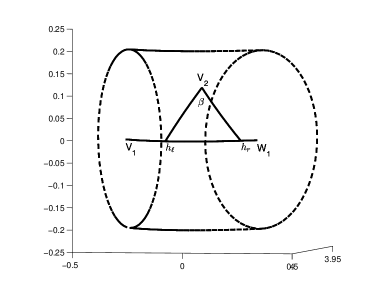
Fig. 5: Feasible domain on the sphere and angle $\beta$ within which $V_{2}W_{2}$ must fall for the arcs $V_{1}W_{1}$ and $V_{2}W_{2}$ to intersect. (When $V_{2}$ is in the right circle (resp. the left circle), $h_{r}$ (resp. $h_{\ell}$) will be at $W_{1}$ (resp. $V_{1}$).

We need several functions in order to calculate $G_{s}(\theta_{1},\phi_{1},\alpha_{1})$:

• The geodesic distance function between two points $P_{1}=(\rho,\theta_{1},\phi_{1})$ and $P_{2}=(\rho,\theta_{2},\phi_{2})$ on the sphere:

  $$gd(P_{1},P_{2})\overset{def.}{=}$$

  $$\rho\arccos[\sin(\phi_{1})\sin(\phi_{2})(\cos(\theta_{1})\cos(\theta_{2})+\sin(\theta_{1})\sin(\theta_{2}))+\cos(\phi_{1})\ cos(\phi_{2})].$$ (39)

• If $X$ and $Y$ are two vectors (in Cartesian coordinates) on the sphere of radius $\rho$, then the normed tangent vector at $X$ to the geodesic line between $X$ and $Y$:

  $$\tau(X,Y)\overset{def.}{=}\dfrac{Y-\frac{X^{T}Y}{\|X\|^{2}}X}{\|Y-\frac{X^{T}Y}{\|X\|^{2}}X\|}$$ (40)

• The $Cart(\rho,\theta,\phi)$ function that transforms spherical coordinates into Cartesian ones (Eq. (34)).

Given $V_{2}=(\rho,\theta_{2},\phi_{2})$ in the feasible domain $FD(d_{1},d_{2})$, we let $h_{r}$ and $h_{\ell}$ be the two points on the equator (on the right and on the left of $V_{2}$) that determine the magnitude of the angle $\beta$ within which $V_{2}W_{2}$ must fall for the intersection to occur (Figure 5).

Bearing in mind $V_{1}$ and $W_{1}$ of Eq. (38), the Cartesian coordinates of $h_{r}$ and $h_{\ell}$, considered functions of $V_{2}=(\theta_{2},\phi_{2})$, are

$$h_{r}(\theta_{2},\phi_{2})\overset{def.}{=}$$

$$\left\{\begin{array}[]{ll}Cart(W_{1})\mbox{ if $gd(V_{2},W_{1})<d_{2}$}\\ \rho\left(\cos\left(\theta_{2}+\arccos\frac{\cos(d_{2}/\rho)}{\sin(\phi_{2})}\right),\sin\left(\theta_{2}+\arccos\frac{\cos(d_{2}/\rho)}{\sin(\phi_{2})}\right),0\right)\mbox{otherwise}.\end{array}\right.$$ (41)

$$h_{\ell}(\theta_{2},\phi_{2})\overset{def.}{=}$$

$$\left\{\begin{array}[]{ll}Cart(V_{1})\mbox{ if $gd(V_{2},V_{1})<d_{2}$}\\ \rho\left(\cos\left(\theta_{2}-\arccos\frac{\cos(d_{2}/\rho)}{\sin(\phi_{2})}\right),\sin\left(\theta_{2}-\arccos\frac{\cos(d_{2}/\rho)}{\sin(\phi_{2})}\right),0\right)\mbox{otherwise}.\end{array}\right.$$ (42)

In the new coordinate system, the probability of intersection $f_{s}(\theta_{1},\phi_{1},\alpha_{1},\theta_{2},\phi_{2})$ conditionally on the arc $V_{1}W_{1}$ and on $V_{2}$ depends only on the components $(\rho,\theta_{2},\phi_{2})$ of $V_{2}$ and is denoted $F_{s}(\theta_{2},\phi_{2})$. Given the uniformity assumption for the angle $\alpha_{2}$ at which the second agent leaves $V_{2}$ to go to $W_{2}$, the probability is equal to the magnitude of the angle $\beta$ within which the arc $V_{2}W_{2}$ must fall for the intersection to occur, divided by $2\pi$. The angle $\beta$ is the angle between the tangent vectors at $V_{2}$ in the directions of $h_{\ell}(\theta_{2},\phi_{2})$ and $h_{r}(\theta_{2},\phi_{2})$. The probability of intersection $F_{s}(\theta_{2},\phi_{2})$ is therefore

$$F_{s}(\theta_{2},\phi_{2})=\dfrac{\arccos\left(\tau[Cart(\rho,\theta_{2},\phi_{2}),h_{r}(\theta_{2},\phi_{2})]^{T}\tau[Cart(\rho,\theta_{2},\phi_{2}),h_{\ell}(\theta_{2},\phi_{2})]\right)}{2\pi}$$ (43)

Table 1: Percentage error $100\times\left(\frac{2d_{1}d_{2}/\pi}{I_{s}(d_{1},d_{2},\rho)}-1\right)$ when approximating $I_{s}(d_{1},d_{2},\rho)$ as $2d_{1}d_{2}/\pi$, with $d_{1}=3$ and an illustrative range of values for $d_{2}$ and $\rho$.

$d_{2}\downarrow;\rho\rightarrow$	2	3	4	5
1	$4.866\times 10^{-4}$	$-1.68\times 10^{-4}$	$-2.527\times 10^{-4}$	$-8.471\times 10^{-4}$
2	$1.288\times 10^{-3}$	$5.595\times 10^{-4}$	$9.269\times 10^{-4}$	$6.658\times 10^{-4}$
3	$-1.506\times 10^{-5}$	$7.529\times 10^{-4}$	$9.412\times 10^{-5}$	$8.954\times 10^{-4}$

The double integral $I_{s}(d_{1},d_{2},\rho)$ is now calculated in the new coordinate system by integrating $F_{s}(\theta_{2},\phi_{2})$ over the feasible domain $FD(d_{1},d_{2})$. Because of symmetries the integral $I_{s}(d_{1},d_{2},\rho)$ is the sum of four times the integral over the upper right quarter of the rectangular area of $FD(d_{1},d_{2})$ and of four times the integral over the upper half of the right circle. We thus have

$$I_{s}(d_{1},d_{2},\rho)=4\rho^{2}\int_{\theta_{2}=0}^{d_{1}/(2\rho)}\int_{\phi_{2}=\pi/2-d_{2}/\rho}^{\pi/2}F_{s}(\theta_{2},\phi_{2})sin(\phi_{2})d\theta_{2}d\phi_{2}+$$

$$4\rho^{2}\int_{\theta_{2}=d_{1}/(2\rho)}^{d_{1}/(2\rho)+d_{2}/\rho}\int_{\phi_{2}=\phi(\theta_{2})}^{\pi/2}F_{s}(\theta_{2},\phi_{2})sin(\phi_{2})d\theta_{2}d\phi_{2}$$ (44)

where

$$\phi(\theta_{2})\overset{def.}{=}\arcsin\left(\dfrac{\cos\frac{d_{2}}{\rho}}{\cos\left(\theta_{2}-\frac{d_{1}}{2\rho}\right)}\right)$$ (45)

is the lower value of $\phi_{2}$ when integrating in the right half circle.

Over a wide range of values for $d_{1},d_{2}$ and $\rho$ we found that the relative error made when approximating $I_{s}(d_{1},d_{2},\rho)$ of Eq. (44) as $2d_{1}d_{2}/\pi$ was of the order of $10^{-3}$ to $10^{-5}$ percent. See Table 1 for an example of this relative error for a range of values of $d_{2}$ and $\rho$. In fact the error is so small that it is within the margin of error when calculating $I_{s}(d_{1},d_{2},\rho)$ numerically. The fact that $I_{s}(d_{1},d_{2},\rho)\approxeq 2d_{1}d_{2}/\pi$ combined with Eq. (17) yields the result of (20).

References

- [1] S. Belongie, Rodrigues’ Rotation Formula. From MathWorld, A Wolfram Web Resource, created by Eric W. Weisstein. http://mathworld.wolfram.com/RodriguesRotationFormula.html
- [2] H.C. Berg, Random Walks in Biology, Princeton University Press, Princeton, 1993.
- [3] E.P. Holland, J.N. Aegerter, C. Dytham, G.C. Smith, Landscape as a Model: The Importance of Geometry. PLoS Comput Biol 3(10), (2007), e200.
- [4] G.F. Lawler, Intersections of random walks. Birkhuser, Boston, 1996.
- [5] Y.M. Park, Direct estimates on intersection probabilities of random walks, J. Stat. Physics, 57 (2005), pp. 319-331.
- [6] Y. Peres, Intersection-Equivalence of Brownian Paths and Certain Branching Processes, Comm. in Math. Physics, 177 (1996), pp. 417-434.
- [7] P.H. Roberts, and H.D. Ursell, Random walks on a sphere and on a Riemannian manifold. Phil. Trans. Royal Soc. London, Series A, 252 (1960), pp. 317-356.
- [8] M. Stefanak, T. Kiss, I. Jex, B. Mohring, The meeting problem in the quantum walk, J. Phys. A: Math. Gen. 39 (2006) 14965-14983.
- [9] J. Sunklodas, On the law of large numbers for weakly dependent random variables, Lithuanian Mathematical Journal, Vol. 44, No. 3, (2004), pp. 285-295.
- [10] A. Telcs, The Art of Random Walks, Springer-Verlag, Berlin, 2006.