Population stratification using
a statistical model on hypergraphs

Abstract

Population stratification is a problem encountered in several areas of biology and public health. We tackle this problem by mapping a population and its elements attributes into a hypergraph, a natural extension of the concept of graph or network to encode associations among any number of elements. On this hypergraph, we construct a statistical model reflecting our intuition about how the elements attributes can emerge from a postulated population structure. Finally, we introduce the concept of stratification representativeness as a mean to identify the simplest stratification already containing most of the information about the population structure. We demonstrate the power of this framework stratifying an animal and a human population based on phenotypic and genotypic properties, respectively.

I Introduction

A population stratification problem consist of uncovering the structure of a population of individuals, samples or elements given a list of attributes characterizing them. For example, the design of a zoo require us to understand what is the best way to allocate different animals in different zoo locations depending on their habitat, behavior, and other properties. The traditional approach to tackle this problem is based on a mapping into a network problem blatt96 ; maclachlan00 ; fred03 ; newman07 ; frey07 , where nodes or vertices represent the population elements, the links or edges represent pairwise relations between the elements, and the edge weights account for the degree of similarity or dissimilarity between the corresponding elements.

In several population stratification problems it is clear, however, that the system under consideration is characterized by relationships involving more than two elements. For example the property - mammal - divides the animal population into two groups: non-mammals and mammals, each containing several elements. Hypergraphs can be used to represent associations beyond pairwise relations. A hypergraph is an intuitive extension of the concept of graph or network where the edges are sets of any number of elements. For example, in an animal population, an edge can represent an association between all animals with a given property, all airborne animals for example.

We consider hypergraphs as a suitable mathematical structure to represent a population of elements and their attributes. We introduce a statistical model on the population attributes hypergraph as a mean to solve the inverse problem, finding the population stratification given the population elements and their associations according to certain attributes. We go over technical issues associated with the framework and its application to real examples as well.

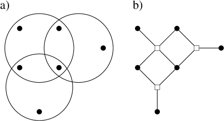
Figure 1: Hypergraph: a) A hypergraph with three edges. Each edge is represented by a circle and its composed by the nodes within the circle. b) Bipartite graph representation of the hypergraph in a), the squares representing the hypergraph edges.

Figure 2: Stratification according to phenotypic attributes: a) A list of animals is given together with certain attributes characterizing them. The complete dataset is available from asuncion07 . Except for the attribute - legs - one and zero indicate possession or not, respectively, of the corresponding attribute. The problem consist on determining the optimal stratification of the animal population based on the provided attributes. b) Hypergraph representing the zoo data. Each line corresponds with an edge, whose elements are specified within the right column. c) ML stratification for the case of eight groups.

Figure 3: Mapping genotypic information into a hypergraph: a) A population of individuals, labeled by 1,2,3…, is given together with their genotype for specific DNA positions within. These positions have been selected because they exhibit significant variation across the human population, referred as single nucleotide polymorphisms (SNPs), and are labeled using the standard SNP notation: rsNUMBER. The letters A, C, G and T represent nucleotides and two letters are reported because each DNA position appear in two different chromosome copies. b) Hypergraph representing the genotypic data. Each line corresponds with an edge, whose elements are specified within the right column.

II Hypergraph representation

A hypergraph is an intuitive extension of the concept of a graph or network where the nodes represent the systems elements and the edges (also called hyperedges) are sets of any number of elements (Fig. 1a). This mathematical construction is very useful to represent a population of elements and their attributes. For example, consider the animal population in Fig. 2a together with their attributes: habitat, nutrition behavior, etc. In this case the hypergraph nodes represent animals. Furthermore, we can use an edge to represent the association between all animals with a given attribute: edge1, all non-airborne animals; edge2, all airborne animals, and so on (Fig. 2b).

This mapping is applicable when the attributes are given by genetic information as well. For example, consider a human population for which we know which nucleotides (represented by the letters A, C, G and T) are present at specific chromosomes and chromosomes positions. Since humans have two copies of each gene, we have two letters for each position. A scenario could be the presence of one of the letters A or G at a given position, resulting in the combinations AA, AG and GG. When these combinations appear in a significant frequency in the population they are referred as a single nucleotide polymorphism (SNP). This genetic information can be mapped into a hypergraph. The vertices in the hypergraph represent individuals and the edges now represent groups of individuals with the same genetic information at a given position: edge1, all individuals with call AA for SNP1; edge2, all individuals with call AG for SNP1; and so on (Fig. 3).

III Statistical model

After identifying hypergraphs as a suitable mathematical structure to represent a population and their attributes we focus on determining how to use this information to solve the inverse problem, finding the population stratification given the population elements and their associations according to certain attributes. Our working hypothesis is that i) the population is divided in groups and (ii) the elements of each group are characterized by a different combination of attributes. The later do not exclude the possibility that two groups exhibit one same attribute, being different according to others. These hypotheses are the basics for the following statistical model on hypergraphs:

Data: Consider a population of $n$ individuals and a hypergraph with $m$ edges characterizing the relationships among them. The hypergraph can be specified, for example, using the adjacency matrix $a$, where $a_{ij}=1$ if element $i$ belongs to edge $j$ and it is zero otherwise.

Model: The population is divided into $n_{g}$ groups and let $g_{i}$, $i=1,\ldots,n$, denote the group to which node $i$ belongs. With probability $\theta_{ij}$ an element of group $i$ belongs to edge $j$.

Likelihood: The likelihood to observe the data given this model is

$$P(a|g,\theta)=\prod_{i=1}^{n}\prod_{j=1}^{m}\theta_{g_{i}j}^{a_{ij}}\left(1-\theta_{g_{i}j}\right)^{1-a_{ij}}\ .$$ (1)

In essence the likelihood (1) is a mathematical representation of our intuition about the observation of the hypergraph given a population stratification, i.e. elements of the same group have the same probability to exhibit certain attribute and thus to belong to the edge representing that attribute. In the following we discuss how to determine the best choice of model parameters ($g,\theta$) and $n_{g}$.

The likelihood (1) resembles that introduced in newman07 in the context of finding communities on graphs. Despite the similarity and being a source of inspiration, they are quite different in their interpretation. A hypergraph can be indeed represented by a bipartite graph, with one type of nodes corresponding to the hypergraph nodes and another representing the hypergraph edges (Fig. 1b). In this work we focus, however, on clustering the original hypergraph nodes alone. Therefore, the likelihood in (1) represents a statistical model on a hypergraph. In contrast, a true statistical model on a bipartite graph should attend to cluster both types of nodes, the original hypergraph nodes and the attribute nodes. There are other technical differences. Here we model the stratification encoded in $g$ as parameters, while they were modeled as hidden variables in newman07 . Hence, although similar in form, the likelihood in (1) is different from that in newman07 .

IV Maximum likelihood stratification

The model defined above belongs to the class of finite mixture models maclachlan00 . Thus, we can obtain the optimal stratification using techniques applicable to finite mixture models in general. In particular, we use the well established Expectation Maximization (EM) algorithm dempster77 to determine the maximum likelihood (ML) stratification given a fixed number of groups.

ML stratification: First, we compute the expectation of the log-likelihood ${\cal L}=\log P(a|g,\theta)$ with respect to the probability $q_{ir}$ that element $i$ belongs to group $r$, obtaining

$$E[{\cal L}]=\sum_{i=1}^{n}\sum_{r=1}^{n_{g}}\sum_{j=1}^{m}q_{ir}\left[a_{ij}\log\theta_{rj}+(1-a_{ij})\log(1-\theta_{rj})\right]\ .$$ (2)

Second, we compute the parameters $\theta$ that maximize (2), resulting in

$$\theta_{rj}=\frac{\sum_{i=1}^{n}q_{ir}a_{ij}}{\sum_{i=1}^{n}q_{ir}}\ .$$ (3)

Finally, $q$ is estimated using

$$q_{ir}=\frac{P(a|g,g_{i}=r,\theta)}{\sum_{s=1}^{n_{g}}P(a|g,g_{i}=s,\theta)}\ .$$ (4)

Starting from an initial condition we iterate the equations (3) and (4) until the change of all $q$ elements is smaller than a predefined precision. The EM algorithm always converge to a local maximum of the likelihood, which may o may not coincide with the global maximum. One approach to explore different local maxima, in case they exist, consist on generating different initial conditions maclachlan00 . Here we explore different initial conditions by assigning to the $q$ elements the random initial values

$$q_{ir}=\frac{x_{ir}}{\sum_{s=1}^{n_{g}}x_{is}}\ ,$$ (5)

where $x_{ir}$ is a random number between zero an one. Putting all together, starting from each initial condition, we iterated equations (3) and (4) until the change of all $q$ elements is smaller than $10^{-6}$.

V Best choice of $n_{g}$

A more subtle issue is to determine the optimal number of groups. The standard approach to solve this problem is based on the Occam’s razor principle: provided different models describing the reality with similar accuracies we should select the simplest. In other words, we accept an increase in model complexity only provided we obtain a signifficantly better description accuracy or predictive power. We use the Akaike Information Theoretical Criterion (AIC) akaike74 to quantify model complexity. According to this criterion, the complexity of a model is determined by the number of independent parameters and the best choice of $n_{g}$ is the one minimizing

$$AIC(ng)=-\max_{\{g,\theta\}}{\cal L}+(n+m)*(n_{g}-1)\ ,$$ (6)

where $(n+m)*(n_{g}-1)$ is the number of independent parameters in our statistical model. The first term in the right hand side of (6) quantifies the goodness of the fit and it decreases with increasing $n_{g}$. On the other hand, the second term in the right hand quantifies the model complexity and increases with increasing $n_{g}$. The optimal choice of $n_{g}$ results from the balance between these two opposite contributions.

It becomes clear below that the AIC criterion can result in too conservative estimates of $n_{g}$, forcing us to consider a different approach. Instead of focusing on model complexity we ask the question: given the ensemble of all models with different $n_{g}$ which is the most representative among them? To be more precise we need a measure to compare the degree of similarity between two different population stratifications $S_{i}$ and $S_{j}$, corresponding to models with $i$ and $j$ groups, respectively. We consider the normalized mutual information fred03

$$I(S_{i},S_{j})=\frac{-2\sum_{k=1}^{n^{(i)}_{g}}\sum_{l=1}^{n^{(j)}_{g}}\rho^{(i,j)}_{kl}\log\rho^{(i,j)}_{kl}/\rho^{(i)}_{k}\rho^{(j)}_{l}}{\sum_{k=1}^{n^{(i)}_{g}}\rho^{(i)}_{k}\log\rho^{(i)}_{k}+\sum_{l=1}^{n^{(j)}_{g}}\rho^{(j)}_{l}\log\rho^{(j)}_{l}}\ ,$$ (7)

where

$$\rho^{(i,j)}_{kl}=\frac{1}{n}\sum_{s=1}^{n}q^{(i)}_{sk}q^{(j)}_{sl}$$ (8)

$$\rho^{(i)}_{k}=\frac{1}{n}\sum_{s=1}^{n}q^{(i)}_{sk}\ .$$ (9)

The normalized mutual information equals zero when the stratification $S_{i}$ does not contain any information about the stratification $S_{j}$, becomes one when the two stratifications are identical, and interpolates between zero and one for intermediate scenarios.

For each stratification $S_{i}$ we define stratification representativeness

$$R(S_{i})=\frac{\sum_{j}I(S_{i},S_{j})}{\sum_{j}1}\ ,$$ (10)

the average of the normalized mutual information of all stratifications $S_{j}$ with respect to a given stratification $S_{i}$. The larger is $R(S_{i})$ the more the stratification $S_{i}$ represent the stratification ensemble and thus the name of representativeness. Furthermore, we define the most representative stratification among an ensemble of stratifications as the stratification maximizing $R$. In case there are more than one stratification satisfying this criteria we invoke the Occam’s razor principle and select the one with the lowest number of groups.

Figure 4: Test example: The best choice of $n_{g}$ and normalized mutual information $I$ between the predicted population optimal stratification and the original stratification as a function of the degree $K$. These results are obtained computing the optimal stratification for $n_{g}=1,\ldots,20$ using the EM algorithm with one initial condition. The optimal $n_{g}$ was obtained using the AIC (solid circles), the representativeness criterion (empty squares) and assuming it equal to four (solid triangles). In a) and b) the case study hypergraphs have $n=100$ nodes and $m=10$ edges, while in c) and d) the number of edges is doubled to $m=20$.

VI Test examples

To test the population stratification framework introduced above we need hypergraph examples for which the stratification is already known. The statistical model defined by (1) provides us a straightforward method to generate an ensemble of hypergraphs. Indeed, provided $g$ and $\theta$ we can generate realizations of the hypergraph adjacency matrix using (1). We consider the following ensemble of hypergraphs with $n$ nodes and $m$ edges: (i) The population is divided in $n_{g}$ groups of equal size. (ii) All nodes have the same degree $K$, where the degree is the number of edges to which a node belongs to. (iii) The edges to which the elements of a given group belong to are selected at random among the $m$ edges, controlling that every pair of groups differ in at least one edge. Provided $m>n_{g}$ the later is possible only for $1\leq K\leq m-1$, defining our working range for $K$.

Using this hypergraph ensemble we generate hypergraphs with $n$ nodes, $m$ edges and degree $K$. For each hypergraph we determine the best choice of $n_{g}$ and the corresponding population stratification, using both the AIC and representativeness criteria. To compare the predicted optimal stratification and the original subdivision of the population we use the normalized mutual information (7) fred03 . Finally, the results are averaged over 100 hypergraps for each set of ($n,m,m$).

Figure 5: Representativeness plot: Representativeness as a function of the number of groups for the zoo a) and MDM4 b) problems. Different symbols indicate different numerical accuracies of the numerical algorithm to find the ML stratification. The arrow indicates the number of groups maximizing the representativeness. The different symbols indicate different number of initial conditions for the EM algorithm, from 100 (open symbols) to 10,000 (filled symbols).

Figure 4 show the results for $n=100$, $m=10$ and $m=20$ as a function of the degree $K$. When we fix, a priori, the number of groups to four, the stratification method based on (1) is almost finding the right subdivision. Indeed, the normalized mutual information between the predicted stratification in four groups and the original subdivision is very close to one, indicating that most nodes have been allocated to their original groups (solid triangles in Fig. 4b and 4d). While these observation does not exclude the existence of hypergraph instances where the method can fail, it supports its use in real cases.

Next we test the best choice of $n_{g}$ when it is not known a priori. For $m=10$ edges the AIC underestimates $n_{g}$, particularly for small $K$ (Fig. 4a). Consequently, the normalized mutual information between the predicted and original subdivision of the population is quite small (Fig. 4b). This disagreement persist for $m=20$ and small values of $K$, but gets signifficantly improved for $K$ larger than four (Fig. 4c,d). In contrast, the representativenes criterion performs quite well for all the tested parameter combinations. In average it predicts the right number of groups, four, (Fig. 4a) and the normalized mutual information is very close to one (Fig. 4b). Taken together these results indicate that the representativeness criterion performs as well if not better that the AIC. Hence, in the following we restrict to the former approach to select the best choice of $n_{g}$.

VII Real examples

Now we proceed to apply the population stratification framework to real examples. The first example is the zoo problem (Fig. 2a), requiring us to group different animals according to their habitat, nutrition behavior, and other properties (Fig. 2a). In this case the hypergraph nodes represent animals and each edge represents an association between animals exhibiting a given phenotypic attribute (e.g. edge1, all non-airborne animals; edge2, all airborne animals, Fig. 2b).

Figure 2c shows the animal stratification for the zoo problem for the case of eight groups. A quick inspection shows that elements within the same group have indeed a sense of a group. The first three groups contain all mammals subdivided by their habitat and feeding behavior. The remaining groups represent birds, fishes, amphibia-reptiles, terrestrial arthropods and aquatic arthropods (except the scorpion), in that order. A similar stratification is obtained for the case of seven groups, except for groups 1 and 3 that are merged into one group. On the other hand, a stratification into nine groups further split the birds into two groups.

Figure 5a shows the representativeness as a function of the number of groups for the zoo problem. For a small number of groups $R$ increases monotonically with increasing the number of groups, saturating to an approximate plateau at large group numbers. In the later region, there are small variations determined by the numerical accuracy of the algorithm computing the ML stratification for a fixed number of groups. A model with eight groups provide the highest degree of representativeness (Fig. 2c). Once again, a quick inspection is sufficient to realize that, indeed, this represent a natural subdivision of the animal population.

The second real example concerns stratification according to genetic information. It consists of a population of ninety caucasians and the genotype at different SNPs within the MDM4 gene, as reported by the HapMap project hapmap03 . The MDM4 gene plays a key role in the p53 stress response pathway and genetic variations within this gene could potentially result in different predispositions to cancer and/or response to cancer drugs therapy harris05 . Focusing on SNPs with variation among this particular subpopulation we stratify its elements using the method described above. Figure 5b shows the representativeness of the ML stratification as a function of the number of groups. As for the zoo problem, the representativeness increases monotonically for a small number of groups and saturates to a plateau with some variations determined by the numerical accuracy. At five groups we already observe a high degree of representation and eight groups represent the best choice of $n_{g}$ according to the representativeness criterion.

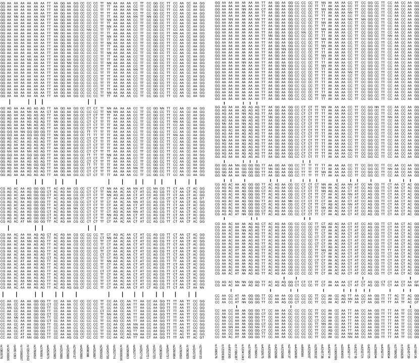
Figure 6: Stratification according to genotypic attributes: A population of ninety caucasians is studied, focusing on SNPs within the MDM4 gene, as reported by the HapMap project hapmap03 . SNPs with no variation within this particular subpopulation have been excluded. A, C, G and T represent the different nucleotides and NN represents data that is not available. The specific SNPs under consideration are indicated by the bottom labels, using the standard SNP notation. The figure shows the ML stratification for the case of five (left) and eight (right) groups, the later corresponding with the best choice of $n_{g}$ according to the representativeness criterion ( Fig. 5b). The vertical lines in between indicate the SNPs at which the adjacent groups differ significantly.

The genetic information for all individuals is shown in Fig. 6 stratified into five and eight groups, the later corresponding with the highest representativeness stratification. The top and bottom groups are almost entirely homozygous (same letter) at every position. In contrast, all the intermediate groups are heterozygous (different letter) at several positions, which do not overlap between them in at least one position. A visual inspection of both stratifications indicates that they are very similar, as anticipated by the close values of representativiness between five and eight groups (Fig. 5b).

VIII Discussion

The mapping of either phenotypic or genetic information into a hypergraph offers significant advantages over the current reductionist mapping of the stratification problem into a network problem. First, the hypergraph contains all the information provided by the original data. Second, it allow us to introduce an intuitive statistical model for the observed phenotypic/genotypic variations based on a postulated population stratification and the tendency of individuals within a group to exhibit certain phenotypic/genotypic feature. Finally, the generalization to problems dealing with both phenotypic and genotypic variation is straightforward, after introducing a hypergraph with two edge types.

The representativeness measure introduced here can be used as an alternative to model complexity when selecting the optimal number of groups given the available information. It is based on the interpretation of statistical significance in terms of information content, a philosophy with increasing recognition among the statistical modeling community fred03 ; slonim05 . This measure allow us to focus our analysis on a stratification obtained for a characteristic number of groups, with a high information content about stratifications with a different number of groups.

Hypergraph partitioning has been already studied with applications to numerical linear algebra and logic circuit design papa07 . The focus has been, however, on balance clustering which aims stratifications on groups of similar size. In contrast, the framework developed here is more suitable to determine a natural partition of the population (or the hypergraph representing it), potentially resulting in clusters of different sizes (see Fig. 1c, for example). It is worth noticing that our framework can be adapted to balance clustering as well, after adding the constraint that all groups have the same size to the starting statistical model.

References

- (1) Blatt M, Wiseman S, Domany E: Super-paramagnetic clustering of data. Phys. Rev. Lett. 1996, 76:3251–3254.
- (2) McLachlan G, Peel D: Finite Mixture Models. John Wiley & Sons, Inc., New York 2000.
- (3) Fred A, Jain A: Robust data clustering. In Proc. IEEE Computer Society Conference on Computer Vision and Pattern Recognition, CVPR, USA, Volume II 2003:128–133.
- (4) Newman M, Leicht E: Mixture models and exploratory analysis in networks. Proc. Natl. Acad. Sci. USA 2007, 104:564–9569.
- (5) Frey B, Dueck D: Clustering by passing messages between data points. Science 2007, 315:972–976.
- (6) Asuncion A, Newman D: UCI Machine Learning Repository 2007, [http://www.ics.uci.edu/~mlearn/MLRepository.html].
- (7) Dempster A, Laird N, Rubin D: Maximum Likelihood from Incomplete Data via the EM Algorithm. J R Statisti Soc B 1977, 39:1–38.
- (8) Akaike H: A new look at the statistical model identification. IEEE Trans. Aut. Control 1974, 19:716–723.
- (9) The International HapMap Consortium: The International HapMap Project. Nature 2003, 426:798–796.
- (10) Harris SL, Levine AJ: The p53 pathway: positive and negative feedback loops. Oncogene 2005, 24:2899–2908.
- (11) Slonim N, Atwal G, Tkacik G, Bialek W: Information based clustering. Proc. Natl. Acad. Sci. USA 2005, 102:18297–18302.
- (12) Papa D, Markov I: Hypergraph Partitioning and Clustering. In Approximation Algorithms and Metaheuristics, CRC Press 2007:61–1–61–19.