Cavity BPM System Tests for the ILC Energy Spectrometer

Abstract

The main physics programme of the International Linear Collider (ILC) requires a measurement of the beam energy at the interaction point with an accuracy of $10^{-4}$ or better. To achieve this goal a magnetic spectrometer using high resolution beam position monitors (BPMs) has been proposed. This paper reports on the cavity BPM system that was deployed to test this proposal. We demonstrate sub-micron resolution and micron level stability over 20 hours for a $1~{}\rm{m}$ long BPM triplet. We find micron-level stability over 1 hour for 3 BPM stations distributed over a $30~{}\rm{m}$ long baseline. The understanding of the behaviour and response of the BPMs gained from this work has allowed full spectrometer tests to be carried out.

1 Introduction

The physics potential of the International Linear Collider (ILC) depends greatly on precise energy measurements of the electron and positron beams at the interaction point (IP). Two types of analysis are particularly sensitive to the collision energy: threshold cross-section measurement and reconstruction of particle resonances [1]. The required accuracy for the mass measurements dictate that the fractional error on the determination of the incoming beam energy must be better than $10^{-4}$. To measure the energy to this level and to minimise the disruption of the beam, a magnetic spectrometer has been proposed.

When passing through a magnetic field, a particle with an electric charge $q$ is deflected by an angle $\theta$ which is inversely proportional to its energy $E$:

$$\theta=\frac{c~{}q}{E}\int{{\it B}\cdot{\rm d}\ell}$$ (1)

where $c$ is the speed of light, ${\it B}$ is the magnetic field and ${\rm d}\ell$ is the path segment along which the particle travels. The initial ILC spectrometer proposal [2] suggested using a single bend and, with careful characterisation of the bending magnets and an accurate measurement of the bend angle $\theta$, the energy of the beam could then be reconstructed.

The performance of a similar spectrometer has already been demonstrated during the second phase of the Large Electron Positron (LEP2) collider at CERN [3]. The magnetic spectrometer installed at LEP2 achieved an accuracy of $1.7\times 10^{-4}$ by measuring the change in bend angle as the beam passed through a single steel dipole magnet. To obtain the high accuracy required, a relative energy measurement was made with the spectrometer calibrated at the $Z^{0}$ resonance using the resonant depolarisation method, thus removing the need for an absolute angle measurement. In order to further improve the accuracy of the measurement, an average was taken over many bunches and many revolutions of the beam around the accelerator. This allowed the requirements on the BPM resolution to be relatively loose.

As the ILC is a linear machine, resonant depolarisation is not an option for the beam energy measurement and in order to limit low energy operation, the ILC spectrometer will have to provide an absolute energy measurement. In addition, a bunch-by-bunch energy measurement is highly desirable to remove some of the dependence on the stability of the machine during physics data taking. These constraints, in addition to the required resolution of the energy measurement ($10^{-4}$), force the performance of the combined BPM and electronics to be considerably higher than the system used at LEP2. In order to achieve this level of performance, high resolution cavity BPMs will need to be used. However, as cavity BPMs are sensitive to the beam slope as well as the beam offset, we are focusing our studies on a different approach to the energy measurement problem from the single bend method initially proposed. Two identical magnets with opposite fields allow the beam energy to be measured as a function of the induced horizontal displacement $x$ given by

$$E=\frac{c~{}q~{}d}{x}\int{{\it B}~{}{\rm d}\ell}.$$ (2)

where $d$ is the total bend length and the deflection angle $\theta$ is small (fig. 1). The inclination of the beam trajectory through the BPMs is then minimised and, by mounting the mid-chicane BPMs on high precision movers, they could be translated to the beam location in the case of large induced offsets.

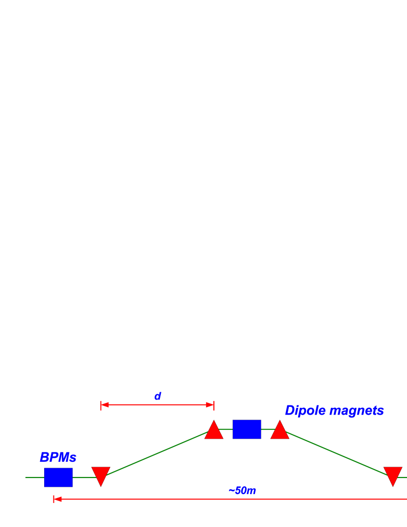
Figure 1: Schematic of the current baseline design for the ILC spectrometer.

The precision and accuracy of the measured offset $x$ contributes directly to the uncertainty of the final energy measurement. The current baseline spectrometer design [4] implements a $5~{}\rm{mm}$ deflection. An offset measurement to better than $500~{}\rm{nm}$ is therefore required to achieve the necessary energy resolution. However, a BPM system with better performance would allow a smaller deflection and, therefore, reduce the emittance growth due to synchrotron radiation. In addition, the system has to be stable to the level of $500~{}\rm{nm}$ over multiple hours to avoid extensive recalibration and consequent loss of luminosity.

The operation and stability of a long baseline BPM system in the proposed spectrometer is of interest in several other fields. For example, the beam position in the ILC linacs must be measured with a resolution of $1~{}\rm{\mu m}$ for the orbit correction and emittance preservation. High resolution BPMs are also required throughout the beam delivery system (BDS). Current test facilities and modern linac based light sources are also demanding significantly better performance from their BPM systems. Most notably, the ATF2 [5] facility at KEK, designed to test the final focus optics for the ILC, not only requires resolutions of $\sim 100~{}\rm{nm}$ for the extraction line BPMs but good stability and ease of use of the entire monitoring system.

In the framework of the T-474 test beam experiment [6] in End Station A (ESA) at the Stanford Linear Accelerator Center (SLAC), we installed several BPM stations in the $40~{}\rm{m}$ available drift space. The aim of three running periods in 2006 was to commission and optimise these BPMs and study their resolution and stability. The principal results of these runs are discussed below.

2 ESA beam and hardware configuration

2.1 Beam delivery to End Station A

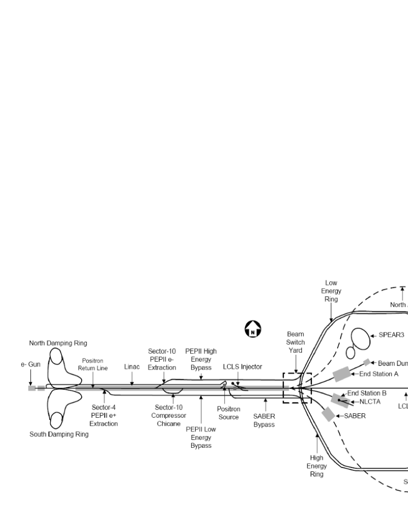
Figure 2: Schematic of the SLAC beam lines that provide a high energy electron beam from the 2-mile SLAC linac, through the Beam Switch Yard to the A-line leading to End Station A.

SLAC’s accelerator and beam transport system for delivering high energy electron beams are depicted in Figure 2. A high intensity electron beam is produced by a thermionic gun, bunched and pre-accelerated in the first sections of the linac to $1.19~{}\rm{GeV}$. The bunches are then kicked by a pulsed magnet into the Linac-to-Ring transfer line and then transported to the electron North Damping Ring (DR), where they are stored for $8~{}\rm{ms}$ to reduce the beam emittance. The Ring-to-Linac transfer line transports the bunches back from the DR and a pulsed magnet kicks them into the linac at Sector 2. The beam is subsequently accelerated to $28.5~{}\rm{GeV}$. At the end of the linac it is then transported from the Beam Switch Yard (BSY) through a $24.5^{\circ}$ bending section into the A-line on its way to End Station A. ESA test beams operate with single bunches at $10~{}\rm{Hz}$ parasitically to PEP-II operation. The ESA is currently the highest energy test beam facility available, with its other beam parameters, listed in Table 1, similar to those for the ILC.

Table 1: Beam parameters at ESA and as proposed for the ILC [7].

Parameter	SLAC ESA	ILC-500
Repetition rate	$10~{}\rm{Hz}$	$5~{}\rm{Hz}$
Energy	$28.5~{}\rm{GeV}$	$250~{}\rm{GeV}$
Train length	up to $400~{}\rm{ns}$	$1~{}\rm{ms}$
Micro bunch spacing	$20-400~{}\rm{ns}$	$337~{}\rm{ns}$
Bunches per train	1 or 2	2820
Bunch charge	$1.6\times 10^{10}$	$2.0\times 10^{10}$
Bunch length	$500~{}\rm{\mu m}$	$300~{}\rm{\mu m}$
Energy spread	$0.15\%$	$0.1\%$

The A-line leading from the BSY to ESA is about $300~{}\rm{m}$ long (see Figure 3). Two BSY dipoles, B1 and B2, just upstream of the D-10 beam dump at the start of the A-line bend the beam through an initial angle of $0.5^{\circ}$, and are followed by a string of 12 dipoles which deflect the beam further by $24^{\circ}$. The quadrupole lattice in the A-line consists of a doublet, Q10 and Q11, at the start of the A-line which brings the beam to a horizontal waist at the dispersion matching quadrupoles, Q19 and Q20. These are located at the high dispersion point (see Figure 4) in the middle of the A-line to correct first- and second-order horizontal dispersion in ESA. Four additional quadrupoles (Q27, Q28, Q30, Q38) near the end of the A-line control the transversal beam size in ESA. The beta functions and horizontal dispersion through the A-line and ESA are shown in Figure 4. Vertical and horizontal corrector dipole pairs, A28/A29 and A32/A33 are used to set the beam trajectory in ESA. They are used in the SLAC Control Program (SCP) feedback to stabilise the beam position at BPM 31 at the end of the A-line and BPM 1 in ESA. SL-10 is a high power momentum slit located at the A-line bend mid-point where the dispersion is at maximum. The maximum momentum acceptance is $2\%$. A SCP energy feedback system uses a stripline BPM, BPM17, at a high dispersion point near SL-10 to stabilise the beam energy.

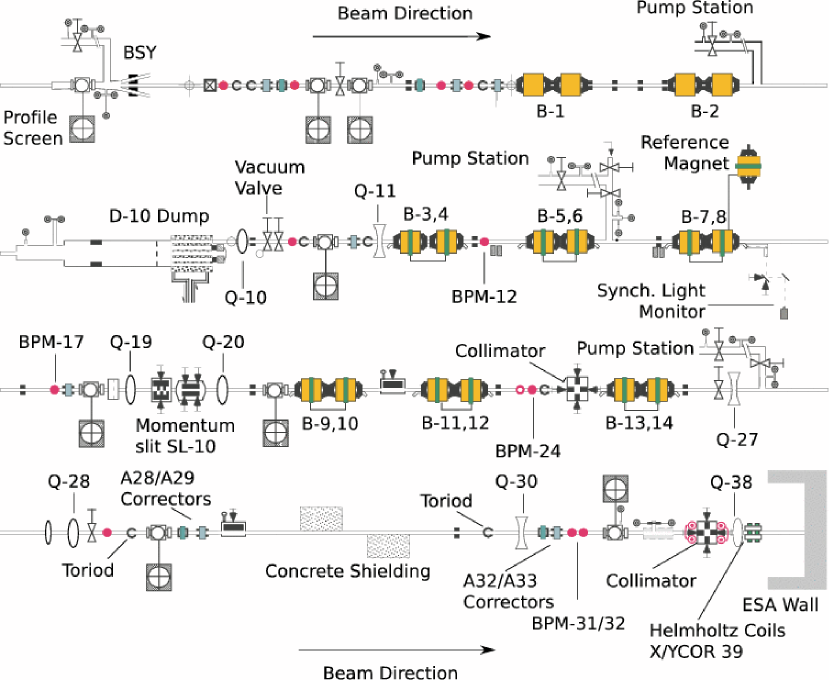
Figure 3: The beam line configuration for the A-line. The beam goes from left to right, top to bottom.

A-line beam diagnostics include RF cavity BPMs, charge-sensitive toroids, a synchrotron light monitor, retractable profile screens, and high frequency diodes. The synchrotron light monitor is positioned upstream of the mid-bend region, and is used to monitor beam energy spread and provide a diagnostic for minimising it. High frequency diodes are installed in ESA for monitoring and tuning the bunch length [8].

Figure 4: The beta functions ($\beta_{x}$, $\beta_{y}$) and horizontal dispersion ($D_{x}$) in the A-line and ESA. The origin is the swivel point in the BSY. The maximum dispersion is at the SL-19 momentum slits in the Aline, as well as the horizontal waist.

2.2 ESA beam line and experimental equipment

The configuration of beam line components, beam diagnostics and experimental equipment at the end of the A-line and in ESA is shown in Figure 5. Two protection collimators are located in ESA; 3C1 ($19~{}\rm{mm}$ aperture radius) is at the entrance to ESA in front of BPM 1 and 3C2 ($8~{}\rm{mm}$ aperture radius) is located in front of BPM 3. There are two beam profile monitors, one upstream of the T480 collimator wakefield experiment (PR2) and one just beyond the east wall of ESA (PR4). These are aluminium oxide screens that can be inserted into the beampipe. Two wire scanners, WS1 and WS2, are approximately $20~{}\rm{m}$ apart and are used to perform transverse beam size measurements. $75~{}\rm{\mu m}$ tungsten wires are scanned across the beam, creating low energy electrons that are detected by photomultiplier tubes at $90^{\circ}$. Several beam loss monitors along the beam line in ESA are interlocked to the machine and radiation protection systems.

Our experimental equipment includes a BPM doublet (BPMs 1,2) and two BPM triplets (BPMs 3-5 and 9-11) and an interferometer system monitoring horizontal motion of the BPM 3-5 triplet. These systems are described in more detail below. Among other experimental setups, a collimator wakefield experiment is located downstream of the BPM 1 and 2 doublet and uses the BPM system for measuring wakefield kick angles [9].

We measured the beam jitter at various BPM stations along the beam line. The typical values for the data discussed in this paper are detailed in Table 2.

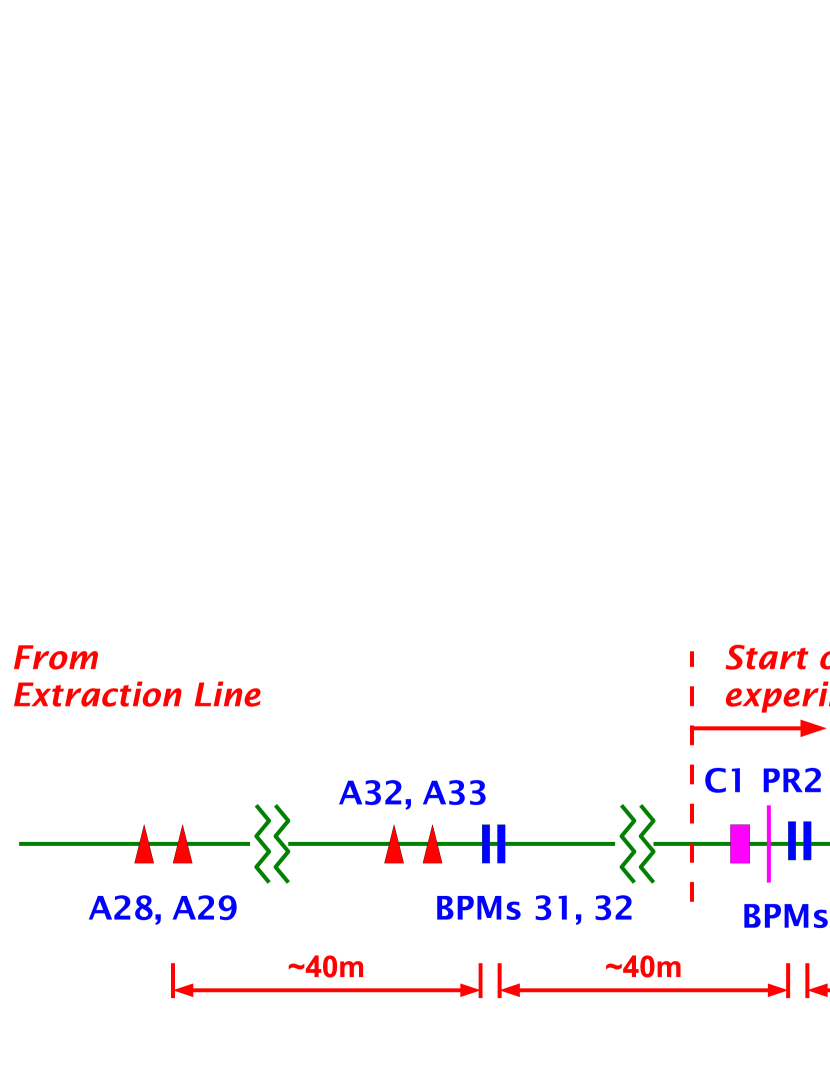
Figure 5: Schematic of the principal beam line components at the end of the A-line and in ESA.

Table 2: The typical beam jitter as recorded at the BPM stations for the data considered in this paper. The error indicates the variation seen over a one hour run.

BPMs	Jitter $x$ ($~{}\rm{\mu m}$)	Jitter $y$ ($~{}\rm{\mu m}$)
1-2	$110\pm 17$	$14\pm 11$
3-5	$157\pm 15$	$40\pm 19$
9-11	$173\pm 16$	$66\pm 22$

2.3 Cavity BPMs

A microwave or Radio Frequency (RF) cavity BPM is a discontinuity in the beam line which, through the excitation of different oscillating electromagnetic field configurations (cavity modes), can be used to measure the position of the transiting bunch. It can be shown that the amplitude of the excited dipole field, providing the bunch is not far from the centre of the BPM, is not only proportional to the charge, but also related to the beam offset $x$ from the centre, the slope $\theta$ of the beam trajectory and the tilt $\alpha$ of the bunch with respect to the cavity [10, 11]:

$$V_{x}\propto xe^{-\Gamma t}\sin{\omega t}$$

$$V_{\alpha}\propto-\alpha e^{-\Gamma t}\cos{\omega t}$$ (3)

$$V_{\theta}\propto\theta e^{-\Gamma t}\cos{\omega t}$$

where the $V$s are contributions to the induced voltage, and $\omega$ and $\Gamma$ are the frequency and the decay constant of the dipole mode. The combined cavity output is given by:

$$V(t) = V_{x}+V_{\alpha}+V_{\theta}$$

$$= e^{-\Gamma t}\left[A_{x}x\sin(\omega t)+(A_{\theta}\theta+A_{\alpha}\alpha)\cos(\omega t)\right],$$

Therefore the position component is always in quadrature with the combined slope and tilt signal and consequently, the angle and position components can be separated providing the beam arrival time is known. For that purpose and also as a bunch charge reference we use additional smaller cavities operating with the monopole mode at the same frequency as the dipole mode in the position cavities. Their signals follow the same processing path as the BPM signals in order to preserve the phase relation.

We used two types of cavity BPMs in our studies: rectangular and cylindrical, all of which have a similar dipole mode frequency. The loaded quality factor $Q_{L}$, which defines the signal decay constant $\Gamma$ via

$$\Gamma=\frac{\omega}{2Q_{L}}$$ (5)

is also similar for all the cavities except for 3, 4 and 5. The general cavity parameters are summarised in Table 3.

Table 3: Parameters of the various BPMs along the ESA beam line. The distances in brackets given for the location are measured relative to the entrance of the experimental hall.

BPM number	Location	Resonant freq.	Loaded $Q_{L}$	Aperture
		(MHz)		(mm)
31, 32	A-Line	$2856$	$\sim 3000$	$51$
1, 2	ESA ($\sim 10~{}\rm{m}$)	$2856$	$\sim 3000$	$51$(1) and $38$(2)
3, 4, 5	ESA ($\sim 25~{}\rm{m}$)	$2859$	$\sim 500$	$36$
9, 10, 11	ESA ($\sim 40~{}\rm{m}$)	$2856$	$\sim 3000$	$20$

Seven rectangular cavity BPMs are available: two in the A-line (BPMs 31 and 32) and five in the End Station (BPMs 1, 2, 9-11). BPMs 9, 10 and 11 were originally designed for use in the main SLAC linac whereas BPMs 31, 32, 1 and 2 were built for the A-Line. Each BPM consists of three separate cavities (see Figure 6a): one cylindrical reference cavity and two rectangular cavities delivering $x$ and $y$ position dependent signals. The rectangular shape of the position cavities helps reduce the effects of coupling between the $x$ and $y$ orientations. We tuned all the rectangular BPMs (including their monopole cavities) to a nominal frequency of $2.856~{}\rm{GHz}$ using external tuners. These BPMs were initially installed for the SLAC E158 experiment [12]. During this installation, BPM 1 suffered significant mechanical damage and as a consequence, both the $x$ and $y$ cavity signals had strong coupling with other modes resulting in worse resolution and stability.

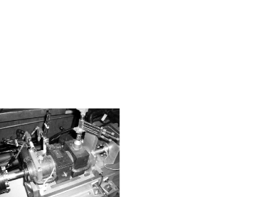
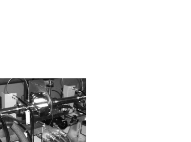
Figure 6: a) An example of the rectangular cavities used for BPMs 31, 32, 1, 2, 9, 10 and 11 showing $x$, $y$ and reference channels and b) the central BPM of the prototype ILC linac BPMs triplet.

The central BPM station (BPMs 3-5) consists of three cylindrical cavities designed for use in the cryogenic regions of the ILC linac (see Figure 6b) [13]. In these BPMs, a single cavity is used to provide both $x$ and $y$ signals. A combination of slots and waveguide couplers provides very good suppression of the unwanted monopole modes. These cavities have a lower $Q$-value and therefore a shorter decay time of the dipole mode signal to provide bunch-to-bunch position measurements in the ILC without the need to exclude the contamination from the previous bunches. We used the reference cavity of BPM 9 to provide the phase and charge information for BPMs 3-5; it was therefore tuned to $2.859~{}\rm{GHz}$.

2.4 DAQ and signal processing electronics

The signal processing electronics that convert the $2.9~{}\rm{GHz}$ signals coupled out of the cavities to low frequency signals prior to digitisation consist of a single stage down-mixing circuit (see Figure 7). The amplitude of the input signal can be adjusted manually with variable attenuators and phase adjustment is also possible. The signal is filtered at the front end with a narrow $20~{}\rm{MHz}$ band-pass filter centred at $2856~{}\rm{MHz}$ to suppress the noise and unwanted modes. No amplification is applied at this stage in order to use the full dynamic range of the mixers. The filtered signal is then mixed with a local oscillator (LO) signal operating at $2939~{}\rm{MHz}$ to produce a low frequency waveform at $\sim 83~{}\rm{MHz}$. An image reject mixer scheme is used to reduce the impact of the unwanted noise and cavity modes around the image frequency. The down-mixed signal is then passed through $20~{}\rm{dB}$ of amplification and an additional $20~{}\rm{MHz}$ bandpass filter.

The electronics for BPMs 3-5 and 9-11 are located close to the beam line, about $20~{}\rm{m}$ from the BPM stations in the experimental hall. The electronics for BPMs 31, 32, 1 and 2 are in a different area (“Counting House”), with an additional $\sim 30~{}\rm{m}$ of cabling required to transfer the high frequency cavity signals to the electronics racks. Also, the signals from BPMs 31, 1 and 2 are split to provide input for the SLAC Control Program (SCP) running the position feedback, adding $6~{}\rm{dB}$ attenuation to these channels.

Digitisation is carried out by four VME Struck SIS330x digitisers, two 12 bit (BPMs 31, 32, 1 and 2) and two 14 bit (BPMs 3-5 and 9-11), with $\pm$2.5 V input range and 50 $\Omega$ input impedance. An external $119~{}\rm{MHz}$ clock signal derived from the linac RF system is used for all the modules. Consequently, the digitiser under-samples the signals, producing a waveform aliased to $\sim 36~{}\rm{MHz}$. Under-sampling is employed in order to widen the gap between the signal peak and image sideband, thus simplifying the hardware filtering at the front end. The digitisers are triggered using a pulse synchronous to the bunch arrival time, which is generated by the linac control system.

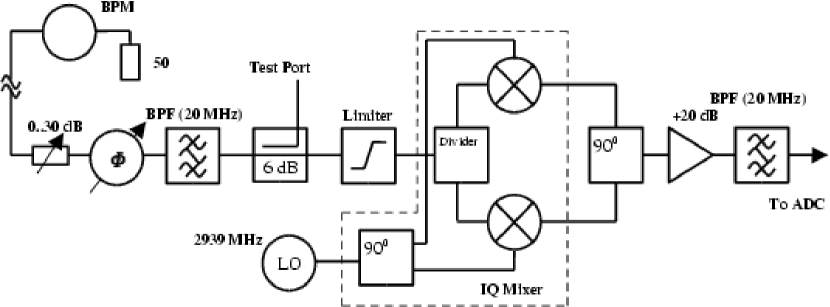
Figure 7: Schematic view of the signal processing electronics. The components within the dashed lines are contained in a single mixer module

The data from the SIS digitisers, as well as that from additional gated Analog-to-Digital Converters (ADCs), VME Smart Analog Monitor (VSAM) and Computer Automated Machine and Control (CAMAC) modules are captured by a Windows XP PC running Labview DAQ programme . In addition to the waveform data, some environmental data are also available such as information on the linac status from the SCP, temperature data from thermocouples placed on the BPMs and electronics, interferometer data (see Section 2.6), stray magnetic field data measured with the flux gate probe and high voltage data for the wire scanners and other experiments. Data are stored at varying rates depending on the source: the waveform data are recorded on a per event basis ($10~{}\rm{Hz}$) with each event corresponding to one bunch being delivered from the linac, but data provided by the SCP and other additional modules are recorded at a significantly slower rate ($\sim 0.1~{}\rm{Hz}$).

2.5 Digital signal processing

The voltage at the front-end of the analogue electronics given by Equation (2.3) can be re-written as:

$$V(t) = Ae^{-\Gamma t}\sin(\omega t+\phi)$$ (6)

where $A=\sqrt{(A_{x}x)^{2}+(A_{\theta}\theta+A_{\alpha}\alpha)^{2}}$ is the amplitude of the waveform and $\phi=\tan^{-1}\left(\frac{A_{\theta}\theta+A_{\alpha}\alpha}{A_{x}x}\right)$ is the phase.

For simplicity, we can assume that the analogue electronics are ideal and only convert the frequency of the waveforms to the first intermediate frequency $\sim 83~{}\rm{MHz}$ so that for both the position and reference cavities we have:

$$V(t) = ae^{-\gamma t}\sin(\omega_{IF1}t+\phi)$$ (7)

$$V_{\rm ref}(t) = a_{\rm ref}e^{-\gamma t}\sin(\omega_{IF1}t+\phi_{\rm ref})$$ (8)

where we neglect the differences of the resonant frequencies and decay constants between the cavities. Note that the decay constant of the signals is changed by the band pass filters.

The waveforms described by Equations (7) and (8) are what appears at the front-end of the digitisers. Due to under-sampling, the frequency of the waveform experiences another conversion to $f_{IF2}=f_{s}-f_{IF1}$, where $f_{s}$ is the sampling frequency of the digitisers ($119~{}\rm{MHz}$ as mentioned above). The amplitude of the resulting waveform remains the same.

In order to extract the amplitude and phase information necessary to recover the position, this waveform is down-converted again in software by multiplying by a complex LO signal at the same frequency as the waveform. This process is called digital down-conversion (DDC). It results in a signal describing the envelope of the initial waveform:

$$V_{\rm DDC}(t) = ae^{-\gamma t}\sin{(\omega_{IF2}t+\phi)}e^{-i\omega_{IF2}t}$$

$$= \frac{a}{2}e^{-\gamma t}\left[-e^{i(\phi+\frac{\pi}{2})}+e^{i(2\omega_{IF2}t+\phi-\frac{\pi}{2})}\right]$$

The mixing process also produces the up-converted component with twice the initial frequency. In order to remove this component and further suppress out-of-band noise, a digital filter is applied. We chose a Gaussian filter as it is easy to implement and has a good phase response within the pass band. Filtering is done in the time domain. As we are interested in the amplitude of the waveform at only one sample point, we reduce the computation time by restricting the filtering to one summation out of the whole convolution:

$$V^{\prime}_{\rm DDC}(t_{0})=\sum_{n=-k}^{n=+k}V_{\rm DDC}(t_{n})\cdot F(t_{n}-t_{0})$$ (10)

where $V^{\prime}_{\rm DDC}$ is the filtered voltage response after down-conversion at the time $t_{0}$, $k$ defines the window of the filter, outside which the contribution is neglected (we set the limit to 0.1% of the maximum filter response), and the filter function is given by:

$$F(t)=\frac{\sqrt{2\pi}\Delta f}{f_{s}}{\rm exp}\left(\frac{-t^{2}(2\pi\Delta f)^{2}}{2f_{s}^{2}}\right)$$ (11)

where $\Delta f$ is the bandwidth of the filter and $f_{s}$ is the sampling frequency.

Applying the filter across all samples we can compute the envelope of the amplitude and the phase for the whole waveform (see Figure 8). A smooth envelope with no oscillations and a flat phase response in the region corresponding to large beam power are an indication of a good frequency determination and low contamination of the waveform with any unwanted signals. The phase variation seen prior to this region is a consequence of the broad-band components of the initial beam excitation.

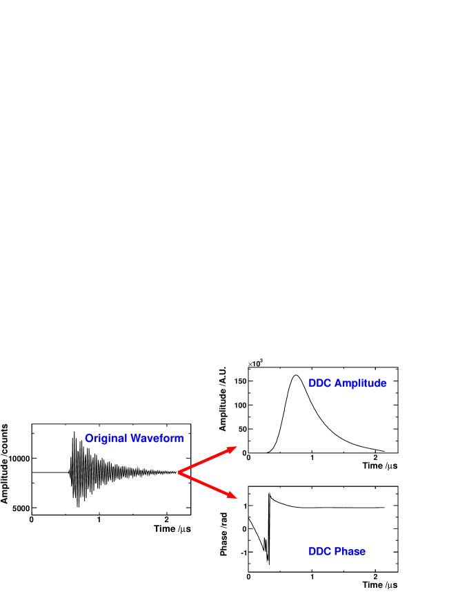
Figure 8: A down-converted waveform as recorded at the digitiser as well as the amplitude and phase response of the DDC algorithm for a whole waveform.

The filtered DDC response depends on the amplitude $a$ and phase $\phi$ of the original digitised waveform:

$$V^{\prime}_{\rm DDC}(t_{0})\propto ae^{i\phi^{\prime}}$$ (12)

$$V^{\prime}_{\rm DDC,ref}(t_{0})\propto a_{\rm ref}e^{i\phi^{\prime}_{\rm ref}}$$ (13)

where $\phi^{\prime}$ includes any phase delays occurring. As mentioned above, the position can be extracted with the help of a reference signal. Normalising the complex amplitude from the position channel with that from the reference channel, we exclude the charge dependence of the position signal:

$$\frac{V^{\prime}_{\rm DDC}(t_{0})}{V^{\prime}_{DDC,ref}(t_{0})}=\frac{a}{a_{\rm ref}}e^{i(\phi^{\prime}-\phi^{\prime}_{\rm ref})}=\frac{a}{a_{\rm ref}}e^{i\Delta\phi}$$ (14)

where the phase offset $\Delta\phi$ between the position and the reference signals at the time $t_{0}$ does not change unless some changes occur in the processing chain.

In order to recover the position information, we need to calibrate the BPMs applying a known offset either to the beam or the BPM. From this we measure the scale $S$ (which is the sensitivity of the term $\frac{a}{a_{\rm ref}}$ to the beam offset) and the phase $\Phi_{IQ}$ (IQ - in-phase/quadrature rotation) of all the points with a positive offset. The position is then given by:

$$x=S~{}{\rm Re}\left[\frac{a}{a_{\rm ref}}~{}e^{i(\Delta\phi-\Phi_{IQ})}\right]$$ (15)

Thus, with an accurate calibration the beam position can be found from the amplitude and phase of a chosen sample of the waveform. The calibration coefficients $S$ and $\Phi_{IQ}$ will only stay accurate for a limited period of time due to gain and phase drifts in the processing electronics and cables, frequency changes of the cavities and other environmental factors. We therefore took calibration data several times during the running period.

In order to optimise the performance of the BPMs and electronics, both the attenuation and alignment offsets of the BPMs needed to be minimised. Initially, with the attenuation set close to maximum to avoid saturation of the waveforms, we measured the relative misalignment of the BPMs from the nominal beam trajectory. Using these data we realigned the BPMs, enabling us to reduce the attenuation. We then repeated this process several times to optimise the sensitivity and dynamic range. The final offset values of the BPMs relative to the mean straight line orbit are shown in Table 4.

Table 4: The relative misalignment of the BPMs with respect to the mean straight line orbit where the error quoted is the error on the mean. The alignment of BPM 4 was optimised continually through the run as it was mounted on the mover system.

BPM	Offset $x$ ($\mu m$)	Offset $y$ ($\mu m$)
1	$-133\pm 3$	$168\pm 0$
2	$-90\pm 3$	$-94\pm 0$
3	$-128\pm 4$	$-193\pm 1$
5	$-134\pm 5$	$10\pm 1$
9	$59\pm 6$	$-60\pm 2$
10	$125\pm 6$	$29\pm 2$
11	$302\pm 6$	$140\pm 2$

2.6 Mover system and interferometer

The middle BPM of the central triplet (BPM 4) is mounted on a dual axis mover system that allows travel in $x$ and $y$ directions. The stages each have a $2~{}\rm{mm}$ pitch lead screw driven by a 200 steps per revolution stepper motor. This gives a resolution of $10~{}\rm{\mu m}$ per step for the BPM moves. The motion system additionally features an LVDT position readout with an accuracy of $\sim 6~{}\rm{\mu m}$. The maximum allowed travel range of the both stages is limited to about $\pm 6~{}\rm{mm}$ for radiation and machine protection reasons. For calibration, a travel distance of $\pm 500~{}\rm{\mu m}$ is used, thus giving a contribution of $\sim 1\%$ to the uncertainty on the calibration scale.

To provide information on the exact $x$ position of BPM 4 and hence allow corrections to the calibration and mechanical position of the assembly, we used a set of three single-pass linear interferometers [14] manufactured by Zygo. Each interferometer measures the relative horizontal displacement of the BPM with respect to interferometer heads on an aluminium table (see Figure 9). A single heterodyne helium-neon laser supplies all three interferometers with polarised light. The interferometer heads are polarised beam splitters that provide the reference and target arms of each of the interferometers with one of the two laser frequencies. Photo-detectors on a Zygo 4004 VME measurement board extract the phase and amplitude of the optical beat frequency present in the recombined light path, allowing a measurement of the relative velocity of the BPMs. The measurement board provides a single bit position resolution of approximately $0.3~{}\rm{nm}$.

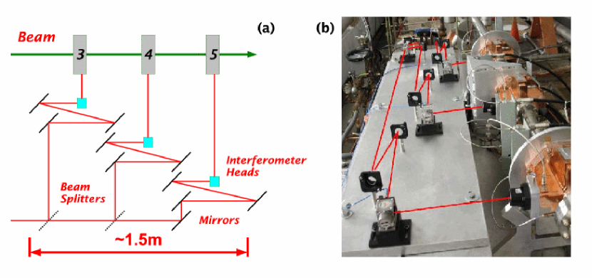
Figure 9: The interferometer system in ESA. a) A schematic of the laser path in the interferometer relative to BPMs 3-5 and the beam line. b) The interferometer elements mounted on the optical table with BPMs 3-5 on the right. The laser path is indicated schematically.

Using the interferometer we measured the vibrational motion of BPMs 3-5. This not only includes the rigid motion of the entire system, but also the non-rigid body motion (i.e. the deviation of each of the individual BPM positions from a straight line) which contributes directly to the measured resolution of the BPMs. The amount of motion recorded at each BPM as well as the non-rigid body motion as extracted from the interferometer data using an SVD method (described in Section 4.1) are listed in Table 5. As BPM 4 is mounted on a non-rigid support, this shows significantly higher vibrational motion than the other two BPMs.

Table 5: Total motion and non-rigid body (NRB) motion measured over 30 minutes in the $x$ direction of BPMs 3-5. The errors quoted are the spread of the RMS.

BPM	RMS (Total)	RMS (NRB)
3	$170\pm 4~{}\rm{nm}$	$94\pm 1~{}\rm{nm}$
4	$680\pm 37~{}\rm{nm}$	$620\pm 10~{}\rm{nm}$
5	$130\pm 3~{}\rm{nm}$	$72\pm 1~{}\rm{nm}$

3 Commissioning of the BPMs

Section 4 will be devoted to the system’s performance during an 18 hour long continuous data taking period which took place at the end of the 2006 running, while in this section we will first report on our studies of the methodology of dealing with BPM signals. More specifically, we will discuss the extraction of the calibration coefficients described in Section 2.5, namely the BPM frequency $\omega$, the phase difference between position and reference signals $\Phi_{IQ}$ and the scale $S$, as well as the optimisation of the DDC algorithm in order to obtain the best resolution and stability of the BPMs.

For the discussion here and the rest of the analysis results we excluded BPM pulses that were saturating the digitisers due to inaccuracies in determining the extrapolation factor.

3.1 BPM frequency and sampling point

The frequency of the digitised BPM signal needs to be measured to a considerable degree of accuracy in order to ensure phase stability when performing the DDC (see Section 2.5). To determine the optimum frequency for each cavity, we fitted the waveforms to an exponentially decaying sine wave using MINUIT [15]. To avoid low amplitude effects, this fit was only performed on events where the beam was driven to large offsets ($\sim 0.5~{}\rm{mm}$, which corresponds to waveforms of approximately half the dynamic range of the digitiser). We combined the fits from all such events over an 18 hour period and took the median in order to get an accurate estimation of the frequency for each BPM throughout the run. The uncertainties associated with these measurements are entirely systematic, due to either physical drift and/or systematic errors associated with the fitting method. We therefore defined the uncertainty on the frequency as the RMS of its distribution. The frequencies determined in this way are listed in Table 6.

Table 6: The frequencies that were used throughout the 18 hour run. The BPMs with errors of zero had a negligible systematic error. The frequency for BPM $11x$ is for the first 8 hours only.

BPM	$f_{x}$ (MHz)	$f_{y}$ (MHz)	$f_{Q}$ (MHz)
1	$36.10\pm 0.06$	$39.47\pm 0.03$	$36.70\pm 0.02$
2	$36.66\pm 0.01$	$36.83\pm 0.01$	as q1
3	$38.46\pm 0.03$	$37.73\pm 0.08$	$39.16\pm 0.01$
4	$39.38\pm 0.07$	$38.85\pm 0.04$	as q3
5	$38.94\pm 0.15$	$39.10\pm 0.04$	as q3
9	$36.53\pm 0.01$	$36.65\pm 0.01$	as q10
10	$36.65\pm 0.01$	$37.29\pm 0.00$	$37.05\pm 0.00$
11	$36.46\pm 0.00$	$36.84\pm 0.01$	as q10

The variation in frequencies seen over the 18 hour period was caused by two different effects. BPMs 3-5 had significantly larger variation than the majority of the remaining BPMs due to systematic effects in fitting waveforms with a short decay time. The number of samples that could be included in the fit was significantly lower than for the other BPMs, thus leading to a larger error. The variation seen in BPMs 9-11 was consistent with being caused by thermal expansion of the cavities. The frequency of a cavity BPM is roughly linearly dependent on the size of the cavity. Assuming a thermal expansion coefficient for copper of $1.7\times 10^{-5}$ per ${}^{\circ}{\rm C}$, a change in temperature of $\sim 0.1^{\circ}{\rm C}$ leads to an expansion of $1.7\times 10^{-6}$, equivalent to $\sim 5~{}\rm{kHz}$ at S-band. Typical frequency variation over the 18 hour period is shown in Figure 10a. The BPM frequency showed a correlation with temperature (see Figure 10b) which is in reasonable agreement with this prediction. Despite having a similar decay time, the variation for BPM 1 was significantly higher than BPMs 9-11 and 2. This was found to be due to interference between different cavity modes as a result of the mechanical damage to the cavity.

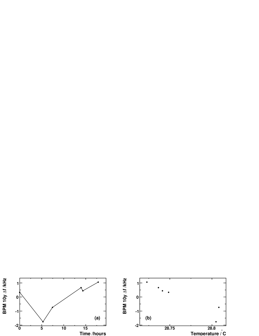
Figure 10: a) The median frequency determined from large offset ($\sim 0.5~{}\rm{mm}$) events over the 18 hour running period for BPM $10y$. b) The fitted frequency versus BPM temperature.

Variations in frequency compromise the calibration and produce an apparent drift and a reduction in resolution if not re-calibrated. Our studies have shown however that induced drifts and resolution deterioration due to frequency changes are small compared to those introduced by other effects (see Section 4).

During the 18 hour period, there was a significant change in the frequency of BPM $11x$ from $36.46~{}\rm{MHz}$ to $36.55~{}\rm{MHz}$. This change occurred during a short access to the experimental hall, so it seems most likely that this was caused by a mechanical disturbance of the cavity or the associated tuner. During the remainder of the 18 hour running, the altered frequency was applied where appropriate.

After we determined the frequency, we could then find the sampling point ($t_{0}$ in Equation 10). This point is defined as the location in the down-converted waveform where we sample the phase and amplitude for the BPM considered. For obvious reasons, the Gaussian filter window is centred around this sample. There is a number of considerations when choosing the optimal sampling point for the analysis including the maximisation of the signal-to-noise ratio, ensuring the sampling point is away from any monopole contamination at the beginning of the waveform and also the phase being constant around the selected sample. We decided to pick a point $10\%$ down from the peak of the filtered waveform (see Figure 8), as a trade-off between the criteria mentioned above. We found the optimum sampling point for each BPM analysing the data containing a large range of the offsets and taking the mean of the resultant sampling point distribution.

Variation of the time difference between the digitiser trigger and the beam arrival time would cause several systematic errors. Firstly, any difference in frequency between the position and reference cavities would make the relative phase sensitive to trigger time variation, thus changing the $IQ$ phase. Though we had attempted to minimise this effect by tuning both the reference and position cavities to the same frequency, differences were still present. Secondly, the trigger time variation would change the relative position of the fixed sampling point with respect to the waveform. This would cause variations in both the recorded amplitude as well as the phase (if the phase was not stable around the chosen sampling point) that would produce apparent changes in scale and $IQ$ phase. As the digitiser was triggered by signals synchronised with the linac timing system, its variation was negligibly small. We determined such variation to be less than a fraction of the digitiser sample by measuring the timing jitter of a reference cavity waveform rectified with a crystal detector.

The only remaining parameter to optimise was the bandwidth of the Gaussian filter used in the DDC algorithm ($\Delta f$ in Equation 11). To determine the optimal value for the filter bandwidth, we calibrated the BPMs and calculated the resolution (as defined in Section 4.1) for a range of bandwidth values. For each BPM station, we used the bandwidth that gave the best resolution for the remainder of the tests (see Table 7). Note that the optimal filter bandwidth scales with the inverse of the cavity fill time, as expected.

Table 7: The filter bandwidth used in the DDC analysis for each set of BPMs.

BPM	Bandwidth ($~{}\rm{MHz}$)
1-2	1.3
3-5	3.8
9-11	1.3
$Q$ cavities	2.8

3.2 Calibration

To measure the remaining calibration coefficients, $S$ and $\Phi_{IQ}$ in Equation 15, we induced a known change in the recorded beam position either through movement of the beam or the BPM. The magnitude of these moves is restricted by the dynamic range of the BPM on the one hand and the beam jitter and short time scale drift on the other hand. We chose typical ranges of $\pm 500~{}\rm{\mu m}$.

3.2.1 BPM calibration with mechanical movers

The most accurate method of calibration available was by means of the mover system on which BPM 4 is mounted. By moving this central BPM of the triplet and using data from the two surrounding BPMs, it is possible to remove the beam jitter and drift from the calibration scan in the central BPM to first order. These three BPMs are also instrumented in the $x$ direction with an interferometer which allowed accurate calibration of the mover system in this axis. As the accuracy of the interferometer is $\sim 5~{}\rm{nm}$, the large moves of $\pm 500~{}\rm{\mu m}$ could be established with a negligible error.

The method used to calibrate BPM 4 with such data was developed by the NanoBPM collaboration [11]. The beam orbit through the three BPMs (3-5) can be considered a straight line in both $xz$ and $yz$ planes. The position in the central BPM can then be predicted from a linear combination of the outer BPM coordinates:

$$x_{k}=\delta_{k}+\sum_{i\neq k}(\alpha_{i}x_{i}+\beta_{i}y_{i}+\rho_{i}x^{\prime}_{i}+\sigma_{i}y^{\prime}_{i})$$ (16)

where $x_{i}$ and $y_{i}$ are the positions recorded in BPM $i$ with the primed coordinates indicating the beam slope values and $\alpha$, $\beta$, $\rho$, $\sigma$ and $\delta$ are constants that encode the relative rotations, offsets, scales and $IQ$ phase differences between the BPMs. As these should not change over short time periods, the same constants can be used to predict the position for many events. Consequently, this relationship can be rewritten in terms of a matrix multiplication:

$$\left(\begin{array}[]{c}x_{k1}\\ x_{k2}\\ \vdots\\ x_{kj}\end{array}\right)=\left(\begin{array}[]{cccccc}1&x_{i1}&y_{i1}&x^{\prime}_{i1}&y^{\prime}_{i1}&\cdots\\ 1&x_{i2}&y_{i2}&x^{\prime}_{i2}&y^{\prime}_{i2}&\cdots\\ \vdots&\vdots&\vdots&\vdots&\vdots&\\ 1&x_{ij}&y_{ij}&x^{\prime}_{ij}&y^{\prime}_{ij}&\cdots\end{array}\right)\cdot\left(\begin{array}[]{c}\delta_{k}\\ \alpha_{i}\\ \beta_{i}\\ \rho_{i}\\ \sigma_{i}\\ \vdots\end{array}\right),\;\mbox{or}\quad{\bf x_{k}}={\bf M}\cdot{\bf K_{k}}$$ (17)

where the $i$ sub-index denotes BPMs 3 and 5 and the $j$ sub-index denotes event number. Thus, to find the constants $\alpha$, $\beta$, $\rho$, $\sigma$ and $\delta$, the matrix of positions above must be inverted:

$${\bf K_{k}}={\bf M^{-1}}\cdot{\bf x_{k}}$$ (18)

To perform the inversion, we employed the method of Singular Value Decomposition (SVD). This involved decomposing the (possibly singular) $M\times N$ matrix into the product of an $M\times N$ column-orthogonal matrix, an $N\times N$ diagonal matrix with positive or zero elements (the singular values) and the transpose of an $N\times N$ orthogonal matrix which could then be trivially inverted. The benefit of this method is that, as no exact solution to Equation 18 is possible due to its over-constrained nature, the least squares minimisation of the equation is found instead. Thus, this method can be used to minimise the BPM residuals by finding the best set of coefficients that can predict the position in the central BPM from the surrounding BPMs.

This method can also provide predictions for the in-phase ($I$) and quadrature ($Q$) components of the signal. First, the positions and slopes of the outer BPMs must be replaced with their measured $I$s and $Q$s in Equation 18. Then the deconvolution and inversion must be carried out twice: once with the position vector (${\bf x_{k}}$) replaced by a vector of the measured in-phase values of the central BPM and the second time with the position vector being replaced by a vector of measured quadrature values.

Assuming the BPM response is linear, the prediction from the outer BPMs to the central BPM is independent of any beam motion that is seen by all BPMs. This includes both beam jitter and beam drift. However, if the central BPM is shifted from its position relative to the outer BPMs, the coefficients would still predict the position at the central BPMs original location. Thus, by comparing the measured and predicted $I$s and $Q$s, the consequence of this move can be seen.

To perform a BPM calibration using this method, we moved the central BPM from $-0.5~{}\rm{mm}$ to $+0.5~{}\rm{mm}$ in 5 steps monitoring the $x$-moves with the interferometer. We then determined the optimum set of coefficients to predict the $I$s and $Q$s at the central BPM using data from the middle step in the calibration (i.e. at zero relative offset). From these coefficients we predicted the $I$s and $Q$s for the rest of the calibration. The mean values for $I$ and $Q$ at each mover position in the calibration were found by fitting the $I$ and $Q$ distributions with a Gaussian function. In the $IQ$ plane these points form a straight line (see Figure 11). As the source of the movement was known to be produced by a position change, this line therefore describes the position axis and consequently, its angle of inclination is equal to the $IQ$ phase ($\Phi_{IQ}$). The resulting predicted position in BPM 4 can then be easily calibrated against the known mover positions, yielding the scale $S$. In order to avoid saturation at the extreme mover positions, we only used the central three steps of the five step mover scan to determine the calibration constants.

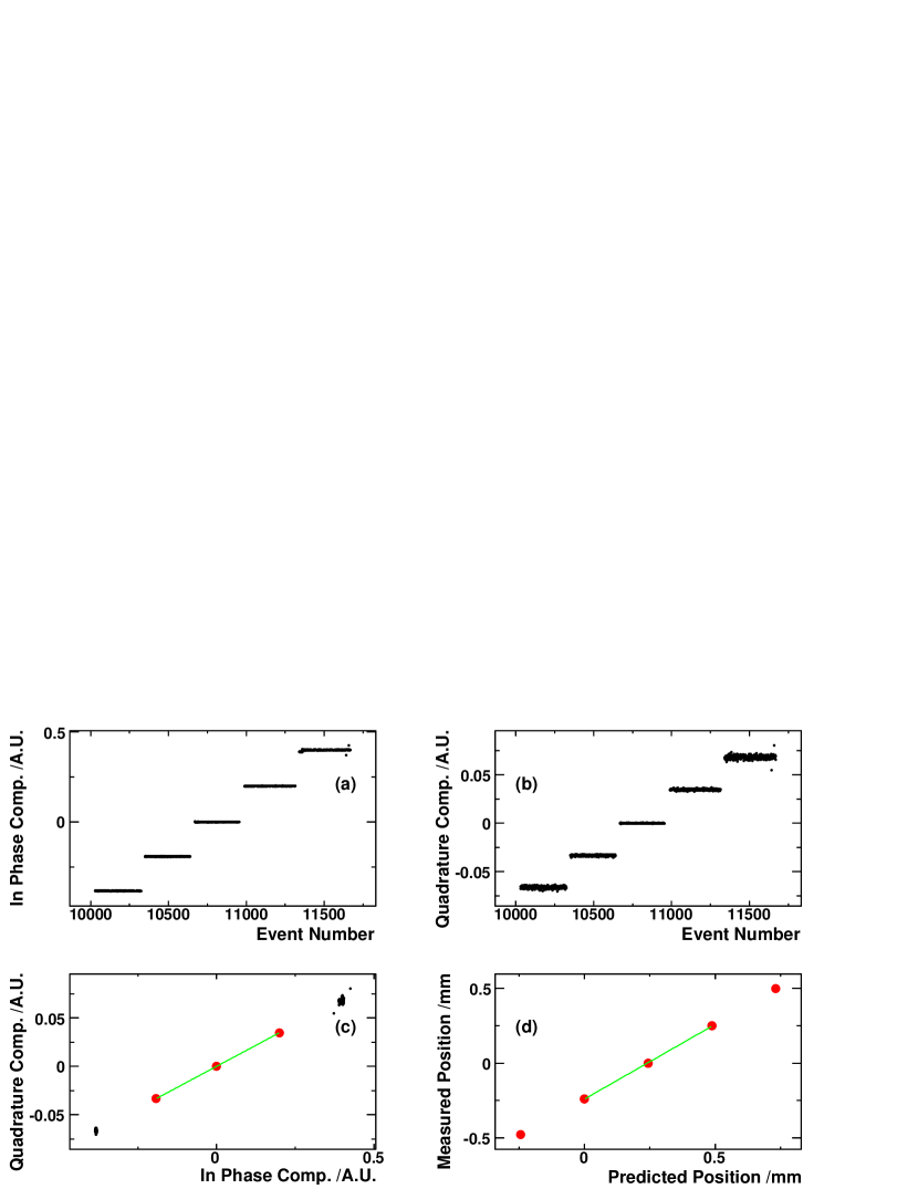
Figure 11: A typical mover calibration. The change of a) the In-Phase ($I$) and b) the Quadrature ($Q$) components against the event number and c) against each other. d) The predicted position against measured position after the calibration.

3.2.2 Corrector scan

To calibrate the remaining BPMs, we varied the integrated field in the correctors A32 and A33 (see Figure 3) from $-0.01{\rm~{}kGm}$ to $+0.01{\rm~{}kGm}$ in five steps. This induced a change of between $\pm 0.5~{}\rm{mm}$ and $\pm 1~{}\rm{mm}$ at the downstream ESA BPMs. We took 60-70 events per step and, for each of these, computed the $I$s and $Q$s. Using the change in $I$ and $Q$ for the various steps, we calculated the $IQ$ phase ($\Phi_{IQ}$) and scale ($S$) as for the mover calibration. Again, only the central three steps were used to avoid saturation.

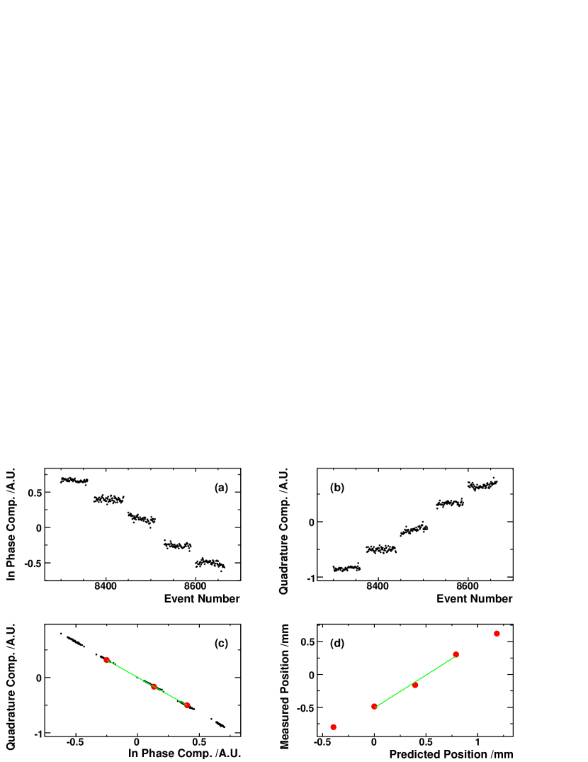
Figure 12: A corrector scan calibration for BPM $10x$. a) The In-Phase ($I$) and b) the Quadrature ($Q$) components against event number, and c) against each other. d) The predicted position against measured position after the calibration.

A significant drawback of this calibration method is that the beam jitter and drift can not be removed by using outer BPMs to predict the position of a central BPM. Though this has little impact on the $IQ$ phase determination, the scale determination is very sensitive to beam drifts, which alter the assumed relationship between the true beam position and the magnetic field in the corrector magnets. In addition, the accuracy of the predicted beam positions was not known as the magnetic field in the corrector magnets was not continuously monitored. The actual changes in beam position could not therefore be determined with sufficient accuracy and this directly contributed to the uncertainty on the scale.

To estimate the improvement in scale determination when using the movers as well as estimate the non-linearities involved, we fitted the predicted versus measured position distribution (see Figure 11d and Figure 12d) with a straight line and found the maximum deviation from the fit. This gave a residual of $\sim 5\%$ for the corrector scan and $\sim 0.5\%$ for the mover scan.

In order to minimise the uncertainty on the scale from drifts during the scan, the more accurate scale for BPM 4 as found from a mover scan was used to correct the BPM scales found from the corrector scan:

$$S^{\prime}_{i}=S_{i}\times\frac{S_{\rm 4,mover}}{S_{4}}$$ (19)

where $S_{i}$ is the scale for BPM $i$ computed using a corrector scan, $S_{\rm 4,mover}$ is the scale for BPM 4 found using a mover scan and $S^{\prime}_{i}$ is the corrected scale. The typical correction factor was of order $15\%$.

4 Experimental results

Having described the methodology of our experiment in the previous sections, we will here report on resolution and stability measurements over short and long periods of operation for the separate BPM stations as well as the complete eight-BPM system over a baseline of 32 m.

4.1 BPM resolution

To measure the resolution of a BPM, we again used the SVD method described in Section 3.2.1 in order to minimise the effect of any calibration inaccuracy on the measurement. The width of the distribution of residuals however contains contributions from all BPMs considered. Considering Equation 16 and making the assumption that the contributions from both the slope and the offset in the orthogonal axis are small we write the width as:

$$\sigma_{k}=\sqrt{R_{k}^{2}-\sum_{i\neq k}\alpha_{i}^{2}R_{i}^{2}}$$ (20)

where $R_{k}$ is the resolution of BPM $k$.

With the further assumption that the predicted position in the residual calculation is defined purely by geometry, the resolutions of all BPMs are the same and the BPMs are equidistantly spaced, Equation 20 reduces to $R_{k}=\sqrt{2/3}\,\sigma_{k}$ for a triplet and $R_{k}=\sqrt{1/2}\,\sigma_{k}$ for a doublet. This correction was applied in the calculation of the individual BPM resolution inside a BPM station. More BPMs can be included, up to the entire set, and the resolution of the reconstructed orbit can be determined. As some of the assumptions above are not valid in this case, we quote the width of the distribution of residuals ”as is” without any corrections and refer to it as the “linked” system resolution. In the energy spectrometer, the precision of the orbit reconstruction in the middle of the chicane directly contributes to the energy measurement. We therefore calculated the residual for BPM 3 in the middle of the baseline versus the rest of the system. The resolutions as recorded during a typical run are shown in Table 8 and an example of a residual distribution is shown in Figure 13.

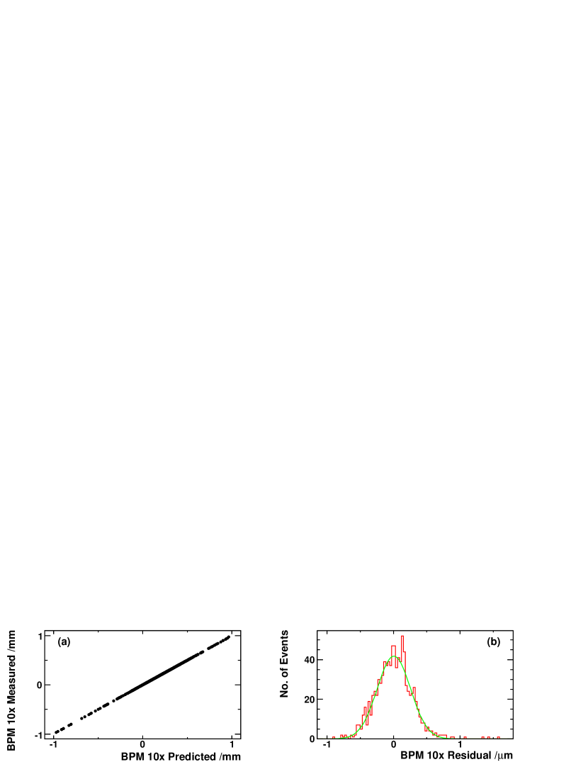
Figure 13: a) The predicted position versus measured position for BPM 10$x$ and b) the residual distribution for the same data.

Table 8: The measured and predicted resolutions of the BPMs in the ESA beam line.

BPM	Measured $x$	Predicted $x$	Measured $y$	Predicted $y$
	($\mu m$)	($\mu m$)	($\mu m$)	($\mu m$)
1, 2	$1.1\pm 0.1$	$1.3\pm 0.7$	$2.2\pm 0.3$	$1.4\pm 0.8$
3, 4, 5	$0.53\pm 0.05$	$0.2\pm 0.1$	$0.46\pm 0.02$	$0.3\pm 0.2$
9, 10, 11	$0.19\pm 0.01$	$0.1\pm 0.1$	$0.17\pm 0.01$	$0.2\pm 0.1$
Linked	$0.82\pm 0.14$		$1.19\pm 0.35$

The main factors contributing to the resolution are electronic noise, digitiser errors and mechanical motion. To estimate the combined RF electronics and digitiser contributions, we ran the DDC algorithm over waveforms that did not contain beam data (i.e. that contained only noise). Dividing the mean of these results by the mean reference amplitude for each BPM and then multiplying by the calibration scale, gave us the predicted resolutions also shown in Table 8.

The measured resolutions for BPMs 1-2 and 9-11 are in reasonable agreement with those predicted indicating that the performance of these BPMs is limited by the combined electronic and digitisation errors. The resolution for BPMs 3-5 is significantly worse than what is predicted but is in reasonable agreement with the amount of vibration recorded by the interferometer (see Table 5) thus indicating that the resolution of these BPMs is limited by mechanical motion. In order to remove this effect, we included the interferometer data in the matrix analysis as additional variables in Equation 16. This addition improved the resolution measurement from $0.53~{}\rm{\mu m}$ to $0.45~{}\rm{\mu m}$ (taking into account the geometric factor), which is equivalent to the removal of $0.35~{}\rm{\mu m}$ of mechanical vibration. This is only half of the non-rigid body motion recorded by the interferometer. High rate ($1~{}\rm{kHz}$) interferometer data indicated that the horizontal vibrational power spectrum peaked between $20-40~{}\rm{Hz}$ (see Figure 14). The latency between interferometer and BPM data arrival acquisition time is of the same order so not all of the mechanical motion could be removed. We plan to remedy this deficiency in future runs.

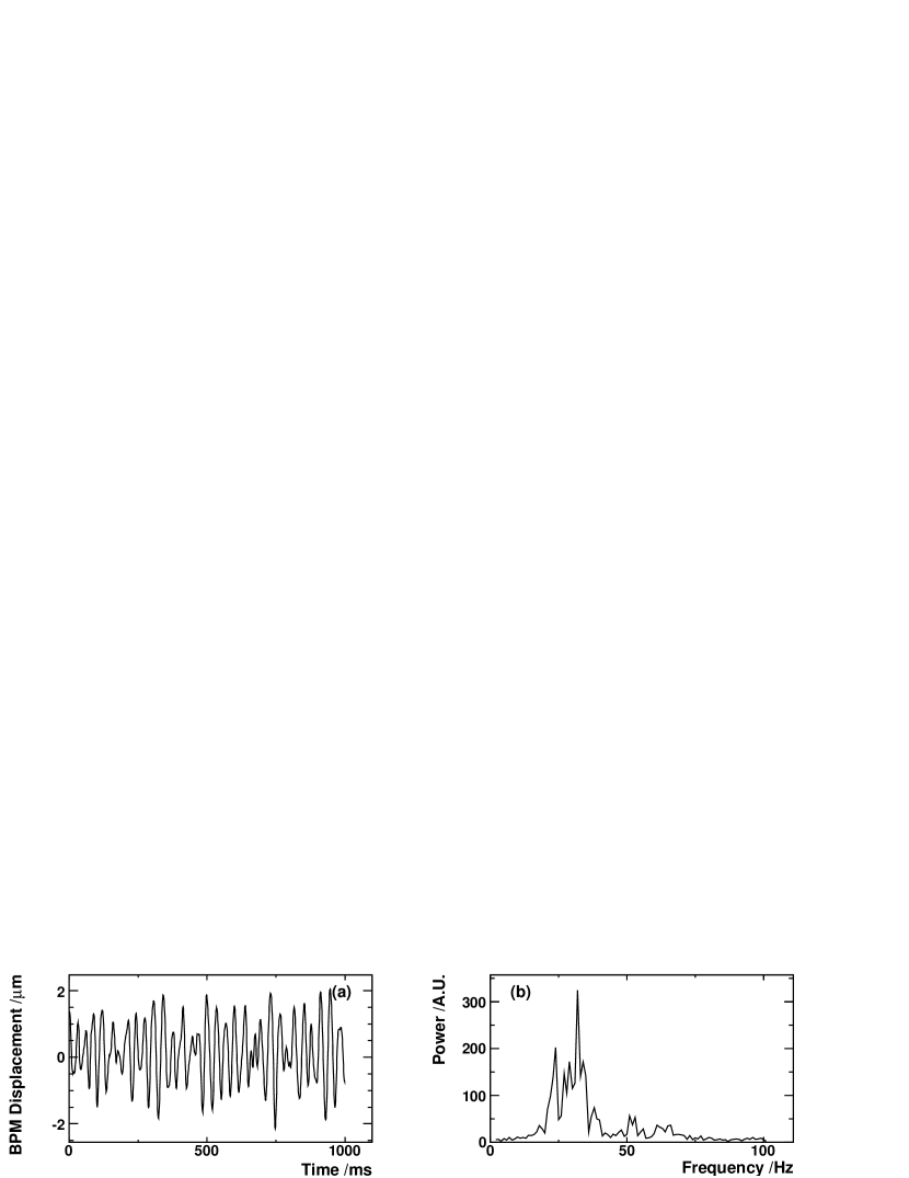
Figure 14: a) The displacement of BPM 4$x$ and b) the power spectrum of the vibrational motion as recorded by the interferometer running at $1~{}\rm{kHz}$.

4.2 Calibration stability

We took several corrector and mover calibration scans over the course of the dedicated 18 hours of operation in order to study the stability of the calibration coefficients. As the parameters of the system vary over time, these coefficients maintain their validity only for a limited period, after which a recalibration is necessary. Understanding of these effects is important for long term stable operation of the BPM system in the spectrometer.

The variation of the calibration constants over the 18 hour running period is shown in Figures 15 and 16. The $IQ$ phase variation is small in all the BPMs except for $1x$ and $11x$. The large phase change in BPM $1x$ was due to a small change in the digitiser trigger time relative to the beam arrival time. Other BPMs are less less sensitive to trigger fluctuations. As mentioned in Section 2.3 however, BPM $1x$ had significant cross-coupling from the vertical mode which resulted in the measured phase being time-dependent. This sensitivity produced a large change in $IQ$ phase during the first calibration run and so this calibration for BPM $1x$ was not used. The large changes in both $IQ$ phase and scale for BPM $11x$ are the result of the perturbation already discussed in Section 3.1. Though a new frequency was used for this section of the run, there is still some residual change. Consequently, we used a separate calibration (frequencies, $IQ$ phase and scale) for this BPM from the time of the perturbation onwards.

Figure 15: Variation of IQ rotation observed over 18 hours of operation.

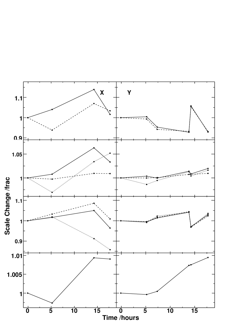
Figure 16: Variation of scale observed over 18 hours of operation.

Apart from those exceptions noted above, the $IQ$ phase for most BPMs indicated a drift of about $20~{}\rm{mrad}$ with no significant difference between the mover and corrector calibration. The scale variation for the BPMs calibrated using the correctors was large despite the corrections of Equation 19. In the $x$ direction, these variations were consistent with the statistical error (about $\pm 4\%$). In the $y$ direction the variation was larger than could be accounted for from beam jitter alone. The scale variations were anti-correlated for the first and third stations which suggested there was a angular variation during the corrector scans with the pivot point somewhere between these BPM stations. Since only BPM 4 was equipped with a mover system, it was only possible to remove offset drifts, not angle drifts, using Equation 19. To measure the slope drift during a calibration run, we used the measured $y$ positions of BPMs 9-11 and BPMs 1 and 2 to calculate the overall slope of the beam and found changes of up to $\sim 3~{}\mu\rm{rad}$. Over the $\sim 20~{}\rm{m}$ of beam line between the central BPM station (3-5) and the outer BPM stations, this leads to a change of $\sim 60~{}\rm{\mu m}$ during a calibration step, introducing a change in scale of $\sim 10-15\%$. This is in good agreement with the $y$ scale variation observed.

The $\mathcal{O}(1\%)$ scale variations observed in the mover calibrations appear to be correlated to the temperature of the electronics racks (see Figure 17). To further test whether environmental effects were behind the gain variations in the electronics, we applied a constant CW tone to the electronics for both the dipole and reference cavities and tracked drifts in relative amplitudes over the course of several hours. A variation of similar magnitude was found from these tests.

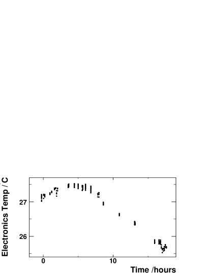
Figure 17: The temperature at the electronics racks in the experimental hall during the 18 hour run.

As the variation in $IQ$ phase was small and the large scale changes seen in the corrector calibrations seem to be caused by the beam drifts rather than electronics drifts, we averaged the coefficients obtained from the separate calibrations and used the mean values for the entire 18 hour run. The only exceptions to this were BPM $1x$ in which the first calibration was removed from the average and BPM $11x$ where two calibrations were used, one computed from calibrations before the mechanical perturbation and the other from after it.

4.3 Stability of BPM offsets and resolution

We investigated the stability of the BPM system over both short and long periods of operation. In both cases the calibration was refined using the SVD over the first 1000-event block of the data. The 1 hour data shown in Figure 18 is a zoom into the last hour of the 18 hour run (Figure 19) after recomputing the SVD coefficients. We had to select the periods of stable data-taking excluding the data taken during the machine tuning, big energy jumps due to klystron failure etc. as well as the calibration data. In addition, due to the perturbation of BPM $11x$, the SVD coefficients for BPMs 9-11 were recomputed.

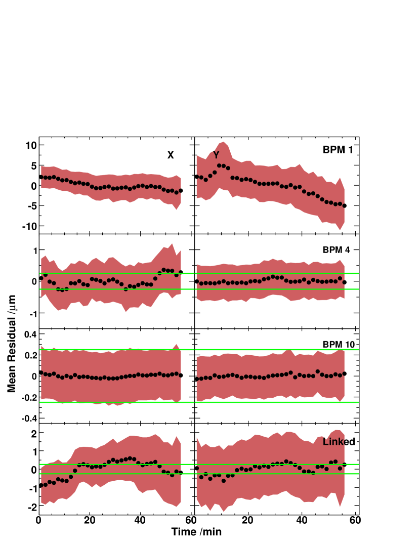
Figure 18: The RMS and mean residual measured in different BPM stations and for the whole system over 1 hour of operation. Each point corresponds to 1000 events.

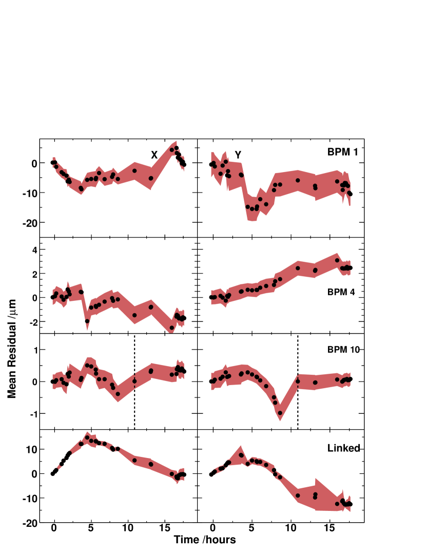
Figure 19: The RMS and mean residual measured in different BPM stations and for the whole system over 18 hours of operation. Each point corresponds to 1000 events. The dotted line indicates where the SVD coefficients were recomputed due to the perturbation of BPM $11x$.

A 100 nm stability of BPMs 9-11, 500 nm of BPMs 3-5 and micron stability of the full system are observed over one hour of operation. The limiting factor for the system’s stability is the stability of BPMs 1 and 2, the electronics for which was exposed to large temperature variations.

For all the BPM stations, the RMS of the residual does not show any significant change with time over the course of the 18 hour run. In contrast, the mean residual experiences large variations, especially for BPMs 1 and 2, and therefore for the linked system as well. We considered the most likely source of these drifts to be gain variations in the electronics. This is supported by Figure 20 where we show the BPM 4 mean residual versus electronics temperature for events in which the beam position in BPM 4 was within $\pm 25~{}\rm{\mu m}$ from the mean position over the course of the 18 hour run. Though there is a change in behaviour at temperatures above $27^{\circ}$C, below this value a significant correlation is seen.

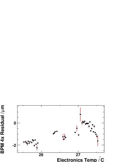
Figure 20: Residual of BPM $4x$ against electronics temperature. Events within $\pm 25~{}\rm{\mu m}$ of the mean position over 18 hours of operation are shown.

To estimate the behaviour of a triplet of BPMs when subject to changes in scale, we simulated three BPMs with offsets typical in our system and a beam orbit experiencing typical beam jitter and drifts. A scale simulated scale drift of $1\%$ was implemented, similar in size to the effects seen in the experiment. We looked at two scenarios: only the central BPM’s scale drifting only (see Figure 21a) and all three BPM scales drifting by the same amount and in the same direction (see Figure 21b). In the first case, both the RMS value and the mean of the apparent beam residual increased gradually, while in the second simulation the RMS value remained almost the same, while the offset increased gradually. The second case is consistent with the effects observed in our system: the physical offsets of the BPMs with respect to each other reconstructed by temperature-dependent gains, resulting in observed changes in the reconstructed offsets.

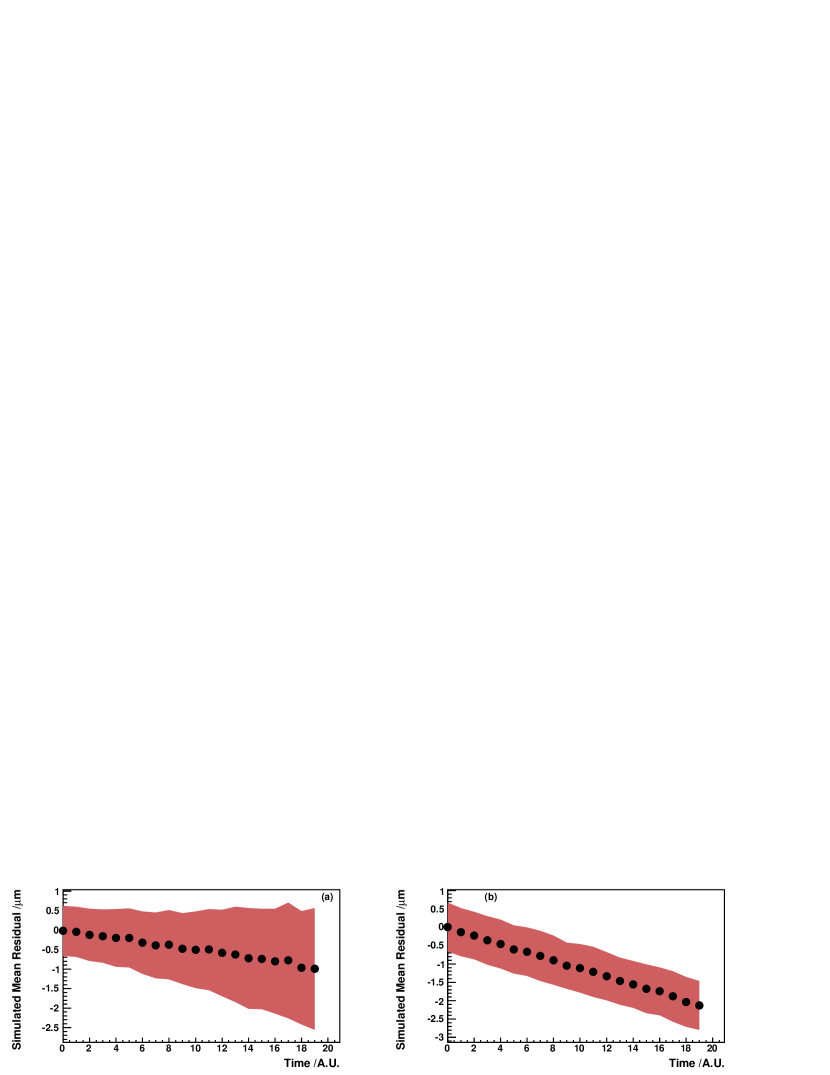
Figure 21: Mean residuals from a simulated BPM triplet experiencing a $1\%$ scale change in a) the central BPM, b) all three BPMs.

We tried improving our stability studies for the central BPM station including the interferometer data into SVD computations. Unfortunately this effort failed as the drifts over long periods of time observed in the interferometer seem to be caused by the thermal expansion of the supporting aluminium table and the change of the refractive index of the air rather than the actual mechanical motion.

We noticed that the residual shows some correlation with the position for low amplitude signals when the beam is close to the cavity centre (see Figure 22), which can be caused by contributions from other cavity modes. This effect is small, but may contribute to the observed main residual variation.

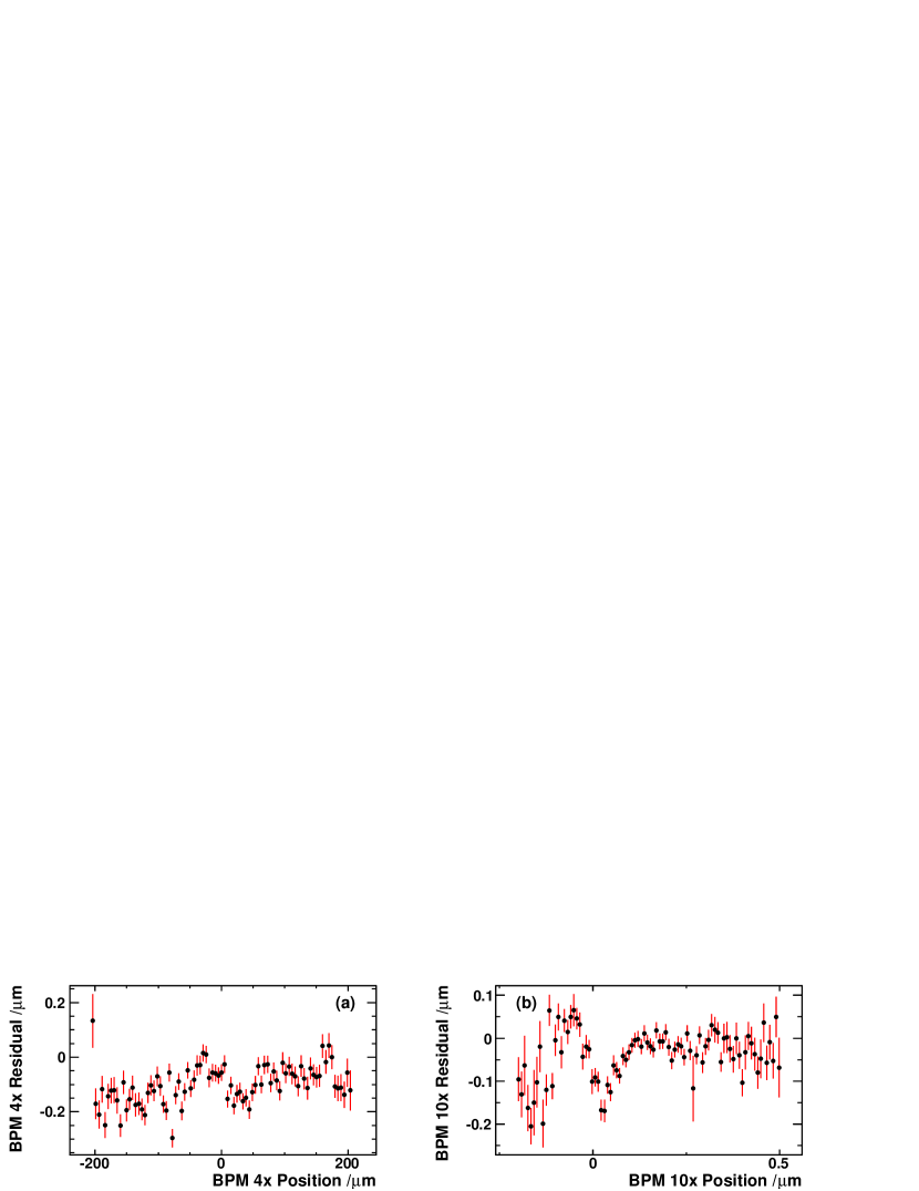
Figure 22: a) The residual between the BPM 4$x$ position measured and predicted with BPMs 3 and 5 over the course of 1 hour against BPM 4$x$ position. b) The residual between the BPM 10$x$ position measured and predicted from BPMs 9 and 11 over the course of 1 hour against BPM 10$x$ position.

The drifts seen in the linked system seemed to be dominated by the scale changes. However, over the long baseline, it is possible that variations in energy combined with the Earth’s Magnetic Field produce a similar effect. To check this the energy of the beam was changed from $-150~{}\rm{MeV}$ to $+250~{}\rm{MeV}$ in five steps. This scan was tracked by the system as a change of the linked system mean residual (Figure 23).

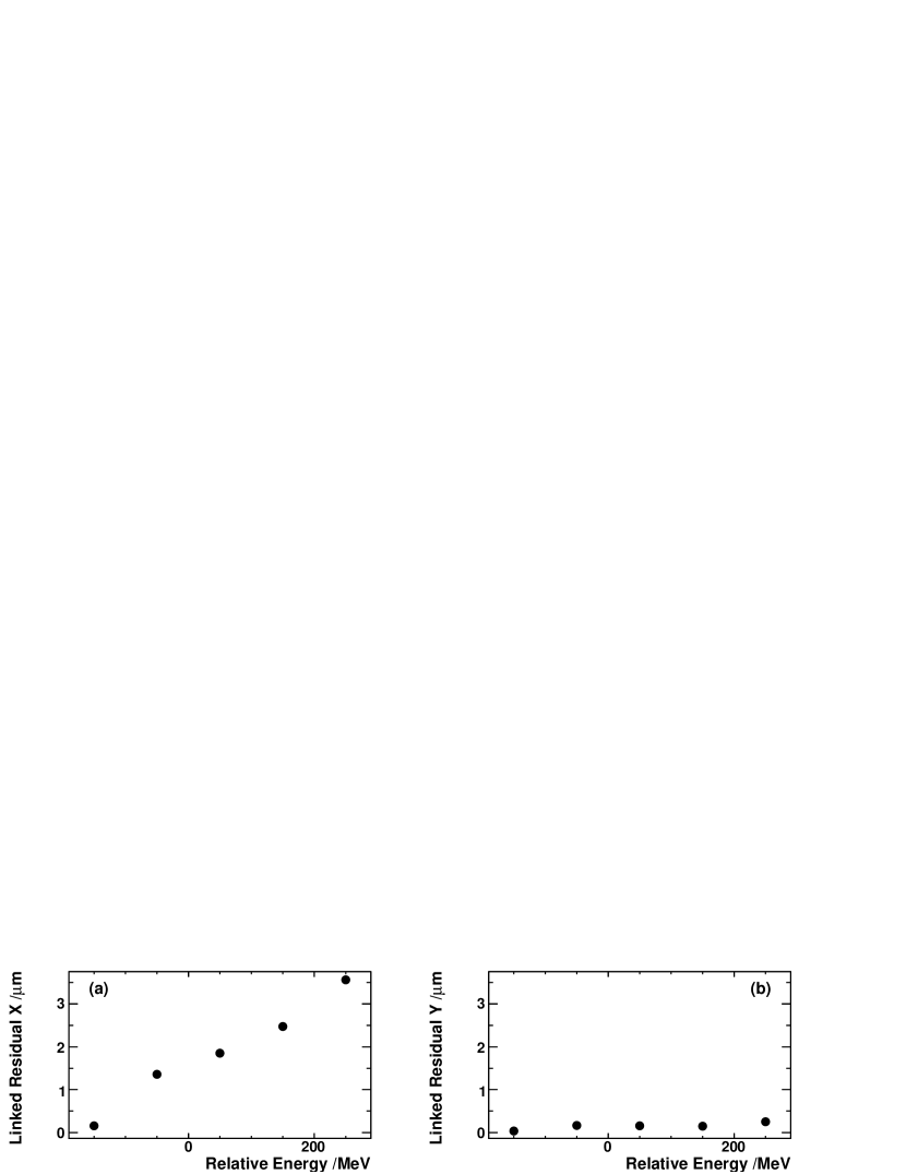
Figure 23: The residual distribution of the linked system at various beam energies.

Using a set of flux gate magnetometers, we measured the stray magnetic fields present around the beam line. Using the measured fields, a change in position of $3.1~{}\rm{\mu m}$ in $x$ and $0.1~{}\rm{\mu m}$ in $y$ is predicted for the $400~{}\rm{MeV}$ energy change. We measured a change of $\sim 3.5~{}\rm{\mu m}$ in $x$ with no significant change in $y$ observed (see Figure 23) which is in good agreement with the prediction. The energy variation over the 18 hour run was $\sim\pm 100~{}\rm{MeV}$ and so the drifts seen over this time period were not consistent with a change in energy.

5 Conclusions

We have successfully commissioned eight cavity BPMs of differing designs and properties divided into three BPM stations in the End Station A beamline at SLAC. The first BPM station consisted of two rectangular cavity BPMs originally designed for use in the A-line. They demonstrated resolutions in $x$ and $y$ of $1.1~{}\rm{\mu m}$ and $2.2~{}\rm{\mu m}$ respectively and were stable to $\pm 5~{}\rm{\mu m}$ over one hour while drifting by $\pm 10~{}\rm{\mu m}$ over 18 hours of operation. The resolution was limited by digitiser errors and noise. The drifts can be explained by the changes of electronics gains.

The second BPM station consisted of three prototype ILC linac cylindrical BPMs with the central BPM mounted on a dual-axis mover. These demonstrated resolutions of $0.53~{}\rm{\mu m}$ in $x$ and $0.46~{}\rm{\mu m}$ in $y$. Mechanical motion was found to dominate the resolution. These BPMs were stable to $\pm 0.25~{}\rm{\mu m}$ over a period of 1 hour and $\pm 1~{}\rm{\mu m}$ over a period of 18 hours. The stability was influenced by low amplitude effects and mechanical vibration on short time scales and scale changes of $\sim 1\%$ magnitude over long time scales.

The final BPM station in the beamline consisted of three rectangular cavity BPMs, originally designed for use in the SLAC linac. They demonstrated resolutions of $0.19~{}\rm{\mu m}$ in $x$ and $0.17~{}\rm{\mu m}$ in $y$ with a stability of $\pm 50~{}\rm{nm}$ over the one hour period. Long term stability of this station could only be measured over 10 hours due to a perturbation that altered the calibration of BPM $11x$. However, over these 10 hours, the triplet achieved a stability of $\pm 500~{}\rm{nm}$ in $x$ and $\pm 750~{}\rm{nm}$ in $y$. As with BPMs 3-5, we think the stability was limited by low amplitude effects and scale drifts, but there was no information on the mechanical motion available for this triplet.

When combining all the BPM stations to measure the precision of the orbit reconstruction over the whole baseline, a resolution of $0.82~{}\rm{\mu m}$ in $x$ and $1.19~{}\rm{\mu m}$ in $y$ was achieved. The system was stable at the micron level over the course of one hour. The long term stability was affected by relative scale drifts across all the BPMs therefore drifts of the order of $\pm 10~{}\rm{\mu m}$ were observed over 18 hours of operation.

In order to improve the system we had in 2006 and be able to perform full tests of a magnetic spectrometer prototype, we have added several upgrades to the beamline and BPM systems. Four steel core dipole magnets have been installed to form the magnetic chicane with BPMs 3 and 5 now measuring the incoming beam position, BPMs 9-11 measuring the outgoing beam position and BPM 4 having been moved to measure the beam position at the mid-chicane location. To improve the stability of the BPMs, we have added a periodic sine wave calibration tone. This is applied through the BPM electronics at a rate of $\sim 0.1~{}\rm{Hz}$ and allows continuous gain and phase monitoring. This should allow us to track calibration changes online and correct for any variation. The interferometer has been extended to measure mechanical drifts between the new incoming BPM station (BPMs 3 and 5) and the mid-chicane BPM. Helmholtz coils have been installed to quickly dither the beam and therefore reduce the dependence of the calibration procedure on beam drifts. We have commissioned these upgrades during 2007 and are planning to continue in 2008, so we will report on the results in our next publication.

6 Acknowledgements

We wish to thank the SLAC accelerator and End Station A operations and support staff. Our work has been supported by the U.S. Department of Energy under contract numbers DE-AC02-76SF00515 (SLAC) and DE-FG02-03ER41279 (UC Berkeley), by the EC under FP6 “Research Infrastructure Action - Structuring the European Research Area” EuroTev DS Project under contract number RIDS-011899 and by the Science and Technology Facilities Council (STFC).

References

- [1] P. Garcia, W. Lohmann, A. Rasperezea, Measurement of the Higgs boson mass and cross section with a linear e+ e- collider, 2nd ECFA/DESY Study 1998-2001 2227–2235, LC-PHSM-2001-054.
- [2] V. N. Duginov, et al., The beam energy spectrometer at the International Linear Collider, DESY LC Notes, LC-DET-2004-031.
- [3] R. Assmann, et al., Calibration of centre-of-mass energies at LEP2 for a precise measurement of the W boson mass, Eur. Phys. J. C39 (2005) 253–292.
-
[4]
ILC Reference Design Report, Volume 3: Accelerator,
URL http://ilcdoc.linearcollider.org/cms/?pid=1000025 (2007). -
[5]
B. I. Grishanov, et al., ATF2 proposal,
URL http://atf.kek.jp/collab/md/projects/project_atf2.php (2006). -
[6]
M. Hildreth, et al., Linear Collider - BPM-based energy spectrometer,
URL http://www-project.slac.stanford.edu/ilc/testfac/ESA/
projects/T-474.html (2004). - [7] M. Woods, et al., Test Beam Studies at SLAC End Station A for the International Linear Collider, European Particle Accelerator Conference (EPAC 06), Edinburgh, Scotland, 26-30 Jun 2006 (2006) 700–702.
- [8] S. Molloy, et al., Picosecond bunch length and energy-z correlation measurements at SLAC’s A-line and End Station A, Particle Accelerator Conference (PAC 07), Albuquerque, New Mexico, 25-29 Jun 2007 4201–4206.
- [9] S. Molloy, et al., Measurements of the transverse wakefields due to varying collimator characteristics, Particle Accelerator Conference (PAC 07), Albuquerque, New Mexico, 25-29 Jun 2007 4207–4212.
- [10] D. H. Whittum, Y. Kolomensky, Analysis of an asymmetric resonant cavity as a beam monitor, Rev. Sci. Instrum. 70 (1999) 2300–2313.
- [11] S. Walston, et al., Performance of a High Resolution Cavity Beam Position Monitor System, Nucl. Instrum. Meth. A578 (2007) 1–22.
- [12] P. L. Anthony, et al., Observation of parity nonconservation in moeller scattering, Phys. Rev. Lett. 92 (2004) 181602.
- [13] C. Adolphsen, ILC linac R&D at SLAC, European Particle Accelerator Conference (EPAC 06), Edinburgh, Scotland, 26-30 Jun 2006 (2006) 822–824.
- [14] F. C. Demerest, High-Resolution, High-Speed, Low Data Age Uncertainty Heterodyne Displacement Measuring Interferometer Electronics, Meas. Sci. Technol. 9 (1998) 1024–1030.
- [15] F. James, M. Roos, Minuit: A System for Function Minimization and analysis of the parameter errors and correlations, Comput. Phys. Commun. 10 (1975) 343–367.