On the Subpulse Modulation, Polarization and Subbeam Carousel Configuration of Pulsar B1857–26

Abstract

New GMRT observations of the five-component pulsar B1857–26 provide detailed insight into its pulse-sequence modulation phenomena for the first time. The outer conal components exhibit a 7.4-rotation-period, longitude-stationary modulation. Several lines of evidence indicate a carousel circulation time ${\mathaccent 94{P}}_{3}$ of about 147 stellar rotations, characteristic of a pattern with 20 beamlets. The pulsar nulls some 20% of the time, usually for only a single pulse, and these nulls show no discernible order or periodicity. Finally, the pulsar’s polarization-angle traverse raises interesting issues: if most of its emission is comprised of a single polarization mode, the full traverse exceeds 180°; or if both polarization modes are present, then the leading and the trailing halves of the profiles exhibit two different modes. In either case the rotating vector model fails to fit the polarization-angle traverse of the core component.

I. Introduction

Pulsar B1857–26, though discovered early (Vaughn & Large 1970), has heretofore been studied almost entirely by average methods. One of the small group of pulsars with five-component (M) profiles, its aggregate polarization has been investigated over a broad frequency band (Hamilton et al 1977; McCulloch et al 1978; Manchester et al 1980; Morris et al 1980; van Ommen et al 1997; & Gould & Lyne 1998), and no effort to interpret the form of pulsar beams fails to mention it (Backer 1976; Lyne & Manchester 1988; Rankin 1983a, 1986, 1990, 1993a,b; Mitra & Deshpande 1999). Little has been learned, however, regarding its pulse-sequence (hereafter PS) behaviour. Apart from one historical effort to determine its null fraction (Ritchings 1976), only recently did the fluctuation-spectral analyses of Weltevrede et al (2006, 2007; hereafter WES, WSE) identify its 7-rotation-period (hereafter $P_{1}$) modulation. PSR B1857–26 is often compared with other prominent M pulsars, but it is not yet known whether it exhibits profile moding like B1237+25 (e.g., Srostlik & Rankin 2005) or core-component phenomena such as those seen in B0329+54 (Mitra et al 2007).

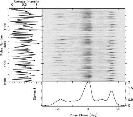
Figure 1: A 200-pulse Stokes-$I$ pulse sequence from pulsar B1857–26 (central panel). The average profile and integrated intensity are given in the bottom and side panels, respectively. Note that the trailing component exhibits a regular 7-rotation-period, longitude-stationary modulation that is also perceptible in the leading component. The intensity scale in this and subsequent figures in arbitrary.

We have carried out a sensitive new 325-MHz polarimetric observation of B1857–26 using the Giant Metre-Wave Radio Telescope (hereafter GMRT) in Maharashtra, and a typical 200-pulse segment is given in Figure 1. Already we see evidence of interesting subpulse modulation. In the remainder of this paper, we describe the results of a series of PS analyses designed to address a number of these questions remaining about this star’s individual pulse behaviour. To our surprise we found that we were able to identify and measure a long period cycle which almost certainly can be interpreted as the rotation interval of an emission-beam carousel in the manner of that found earlier for B0943+10 (Deshpande & Rankin 1999, 2001; hereafter DR99, DR01). Such cycles are thought to be driven by ${\bf E}$$\times$${\bf B}$ forces within a pulsar’s polar flux tube along the lines of the Ruderman & Sutherland (1975; hereafter R&S) theory; however, all those so far determined or reliably estimated are longer or much longer than predicted by the theory. §II describes the GMRT observations, and §III our efforts to measure and model its polarisation-angle traverse, so as to better determine the emission geometry. In §IV we analyse the properties of the nulls, and in §V we outline the dynamics of its core component. §VI gives a discussion the fluctuation-spectral analyses, and §VII the evidence for a tertiary modulation cycle. §VIII then discusses the configuration of the pulsar’s subbeam carousel, and §IX gives a brief discussion and summary of the results.

II. Observations

Pulse-sequence polarisation observations of pulsar B1857–26 were acquired using the Giant Meterwave Radio Telescope (GMRT) north of Pune, India at 325 MHz on 2004 August 27. The GMRT is a multi-element aperture-synthesis telescope consisting of 30 antennas which can be configured as a single dish. The polarimetry discussed here combined the array signals coherently in the upper of the two 16-MHz ‘sidebands’ in a manner identical to that described for pulsar B0329+54 in Mitra et al (2007). The pulsar back-end computed both the auto- and cross-polarized power levels, which were then recorded at a sampling interval of 0.512 msec. A suitable calibration procedure as described in Mitra et al (2005) was applied to the recorded observations to recover the calibrated Stokes parameters $I$, $Q$, $U$ and $V$. The duration of the PS is 19.4 minutes or 1945 pulses. In addition, a total-power observation at 610 MHz with the same bandwidth, sampling time and duration was carried out on 2007 February 4.

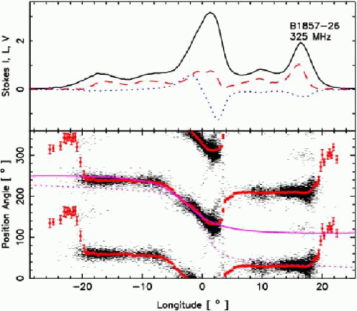
Figure 2: PA histograms for the entire 325-MHz PS. The upper panels show the aggregate total power, total linear and circular polarisation (LH-RH), and the lower panel gives the polarization-angle (hereafter PA) density. The PA values are plotted twice for clarity, and the two curves indicate negative-going RVM fits to the PA traverse. One RVM fit (dotted curve) assumes that both sides of the profile represent the PPM and, clearly, it fails to describe the $>$180°extent of this apparent PA rotation. A second RVM fit assumes that different OPMs predominate in the leading and trailing parts of the profile. The longitude origin is taken near the zero-crossing point of the antisymmetric Stokes $V$ signature.

III. Emission Geometry

A histogram of the polarisation-angle (hereafter PA) behaviour of the 325-MHz observation is given in Figure 2. The upper panel shows the star’s five components in total intensity (Stokes $I$), the total linear polarisation (Stokes $L$ [=$\sqrt{Q^{2}+U^{2}}$]) and the circular polarization (Stokes $V$ [=LH–RH]); whereas the lower panel gives the PA density twice for clarity. Several aspects of this diagram deserve close discussion.

First, the very flat PA curves under the wings of the profile appear compatible with a positive (equatorward) sense of the sightline impact angle $\beta$ as our attempts to fit a rotating-vector model (hereafter RVM: Radhakrishnan & Cooke 1969; Komesaroff 1970) to the traverse bear out. Gould & Lyne’s (1998) polarimetry confirms this aspect of the pulsar’s PA traverse at meter wavelengths. At 1.4 GHz, however, the traverse under the wings of the profile is not at all flat and even shows different slopes on the leading and trailing sides of the profile (see also Johnston et al 2005). Clearly, such behaviour is difficult or impossible to reconcile with the RVM.

Second, no sensible RVM fit could be obtained to the PA traverse under the assumption that most of the star’s emission, throughout the profile, stems from a single orthogonal polarisation mode (hereafter OPM)—here the putative primary polarization mode (hereafter PPM). All the published observations seem to confirm that the PA traverse rotates negatively (clockwise) in the center of the profile, but if most of the emission reflects the PPM, then the full PA traverse significantly exceeds 180° both at meter and centimeter wavelengths. While the RVM PA excursion can exceed 180°for inner (poleward) sightline traverses, it cannot do so for outer ones, thus some different interpretation is needed. This difficulty is illustrated by the fit (dotted curve) in the bottom panel of Fig. 2.

Figure 3: Longitude-resolved fluctuation spectra for pulsar B1857–26 at 325 (top left and right) and 610 (bottom left) MHz. The full spectra are shown in the main panels, the integral spectra (for the outer components only) in the lower ones, and the side panels give the average profiles (along with the dashed boundaries for computing the integral spectra). Most intervals of the PSs exhibit a bright narrow feature (top left, full 1900 PS) at 0.14 c/$P_{1}$ or a $P_{3}$ value of some 7.4 $P_{1}$, whereas others show disorderly, weaker responses (right, pulses 1-600) which include the 0.14 c/$P_{1}$ feature. The first 600 pulses of the 610-MHz PS (bottom left) exhibit a strong low frequency periodicity as well as ‘sidebands’ adjacent to the primary modulation feature. Here overlapping ffts of length 256 were used.

We also tried to fit B1857–26’s PA trajectory making the somewhat unsavory assumption that different OPMs are dominant in the leading and trailing wings of the pulse profile (as we know of no excellent example of this configuration in other pulsars). This RVM fit is indicated by the thinner full curve in Fig. 2, and note that it is hardly excellent. It results in a large (some 3°) displacement between the PA inflection point and the zero-crossing longitude of the circular polarization.

One characteristic of the profile possibly supporting this interpretation is the deep minimum in the total linear polarization just following the core component, which is prominent in every published observation. This latter fit results in values for the magnetic latitude $\alpha$ and sightline-impact angle $\beta$ of 155 and –1.8°, respectively (using the Everett & Weisberg [2001] convention)—or equivalently an outer traverse with $\alpha$, $\beta$ some 25, +1.8°.

Finally, B1857–26’s absolute fiducial PA orientation was determined by Johnston et al (2005) and also discussed by Rankin (2007), so it is important to understand the geometry of the pulsar’s OPM emission. The two RVM fits (as well as the further conjecture) above make very different assumptions about this geometry, and they result in different offsets between the centres of the linear and circular polarisation. Further study at multiple frequencies is needed to resolve these issues; but, fortunately, we need not settle them fully for our present purpose.

IV. Nulling Behaviour

B1857–26 exhibits some 20$\pm$3% null pulses, substantially more than the 10$\pm$2.5% indicated by Ritchings’ (1976) very old analysis. We computed null histograms for the observations similar to Redman et al’s fig. 12. In both, the pulsar maintains a relatively constant brightness (so scintillation effects are minimal) and the noise level is such that about 0.3 $<$$I$$>$ provides a plausible threshold for null identification. The intensity distributions of the pulsar signal and noise overlap so that weak pulses cannot be reliably distinguished from nulls. Nonetheless, we see that the pulsar’s nulls are very short, with a strong propensity for 1 $P_{1}$ duration, and a maximum length in our observations of 4 $P_{1}$. Its bursts are also short, many having only a single period, and a mean burst length of only 5 $P_{1}$. We find little evidence that the nulls are non-random or even weakly periodic (using the methods of Herfindal & Rankin 2007). However, the average profile of the putative nulls (not shown) does indicate significant power at the longitude of the central component, whereas the partial profiles of pulses just before and just after nulls show no significant difference in form from the total average profile.

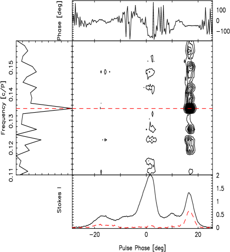
Figure 4: Modulation amplitude (bottom panel dashed curve) and phase (top panel) for the pulse 1101-1612 sub-PS in Fig. 3 (top left), shown as a function of the average-profile power (solid curve bottom panel). The central panel shows the contour levels for the lrf (zoomed in between 0.08 to 0.2 c/$P_{1}$) and the left panel shows the longitude-averaged fluctuation spectrum. Note that virtually all of the fluctuating power here falls under the outer conal component pair (I & V)—and primarily V.

V. Core Dynamics

The PS properties of core-component emission have not been well studied, and B1857–26 provides a further important opportunity to examine its characteristics. This pulsar’s core tends to be quite regular in intensity, as is suggested by Fig. 1 and further indicated by its rather small modulation indices at both 92 and 21 cms (WES, WSE). The core feature is not at all symmetrical (or of Gaussian form) with its slow rise and steeper fall, and its constituent subpulses exhibit neither the intensity-dependent form nor the longitude shift seen in pulsar B0329+54 (e.g., Mitra et al 2007). Even its antisymmetric circular polarisation is rather consistent, showing very nearly the same phase in every pulse. Interestingly, the strongest single pulses seem always to fall near the core peak and are highly left-hand circularly polarised; whereas the leading right-hand circular is somewhat weaker and steadier (see also WSE’s asymmetric variance profile). Also, we see a slight change in the total linear polarisation from a double form at low intensities to an emphasis on the trailing lobe in the strongest pulses. Again, the circularly polarised core signature in B1857–26 bears careful examination as it fails to be fully antisymmetric in just the same manner as the Stokes $I$ profile fails to be symmetric. Nonetheless, its zero-crossing point falls very close to the center of the conal profile.

VI. Fluctuation-Spectral Analyses

Figure 3 gives longitude-resolved fluctuation (hereafter lrf) spectra for three different segments of the two PSs. As expected from Fig. 1 periodic modulation is seen in the outer conal components (I and V, and its contribution is shown in the integrated fluctuation spectra in the bottom panels) which often exhibits a strong feature near 0.14 cycle/$P_{1}$ (hereafter c/$P_{1}$). The 325-MHz lrf (top left) shows that this narrow feature dominates throughout the entire PS. Atop the broader response, its power falls in a single bin of a 512-length FFT (not shown) with a frequency of 0.135$\pm$0.001 c/$P_{1}$ or 7.41$\pm$0.06 $P_{1}$. The corresponding harmonic-resolved fluctuation spectrum (hereafter hrf, see DR01 for details; also not shown) indicates that the respective positive and negative responses represent mostly amplitude modulation as expected. Figure 4 shows the modulation amplitude and phase for the interval 1101–1612 PS. Virtually all the power with this periodicity falls under the outer conal components (not the inner pair), and the flat phase gradient in this region indicates a longitude-stationary modulation—just as expected for a highly central sightline traverse.

Other sections of the 325-MHz PS, however, show less regularity. The right-hand lrf plot of Fig. 3 gives a representative example. Here, the fluctuations produce several broad features around the primary one. We emphasize that the 7-$P_{1}$ modulation is associated with the outer conal components and primarily the trailing one; it cannot even be detected in the inner conal region of the profile. The fluctuation spectra of the outer components is conflated in the integral spectra, but separate analyses (not shown) of the conal and core parts of the profile show that the core contributes little (even noise power) to the integral spectra. In summary, only the outer cone fluctuates significantly at the roughly 7-$P_{1}$ cycle.

The bottom lrf of Fig. 3 was computed from the first 600 pulses of the 610-MHz observation (using overlapping 256-length ffts). It shows both a low frequency feature and two ‘sidelobes’ adjacent to the primary modulation feature, possibly indicating a tertiary modulation as in B0943+10 (see DR01). The primary modulation has a period of some 7.11$\pm$0.01 $P_{1}$, whereas the entire PS gives 7.34$\pm$0.01 $P_{1}$, suggesting that the primary modulation frequency is somewhat variable. The low frequency feature can be measured over an interval of up to 1000 pulses, and the hrf (not shown) indicates that it represents a mixture of amplitude and phase modulation with a period of about 145 $P_{1}$. The two ‘sidebands’ are not equally spaced, but the average interval is about 0.013 c/$P_{1}$.

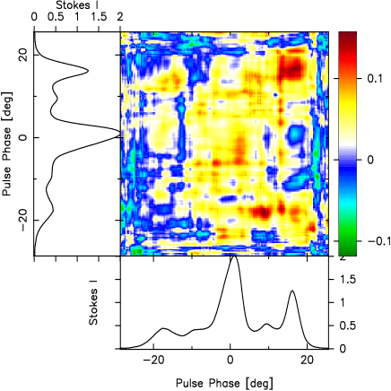
Figure 5: The top plot shows the correlation coefficient of pulses 800-1100 of the 325-MHz PS in Figs. 3 & 4 using only the trailing longitude regions. The bottom display gives the longitude-longitude correlation for a delay of 147 $P_{1}$ over a longer PS of 800-1700. The main panel gives the correlation according to the color bar on the right, and the average profiles are plotted on both axes for reference. The ordinate has been delayed with respect to the abscissa. The 7-$P_{1}$ cycle is clearly seen in top plot. Note, however, the extraordinary peak at 147 $P_{1}$ which shows some 30% correlation in the top plot and is clearly seen in the trailing component in the bottom display.

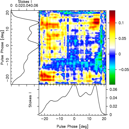
Figure 6: Correlation plots as in Fig. 5 of pulses 800-1900 of the 610-MHz PS using both the leading and trailing components. Note the peak at 147 $P_{1}$. High correlation regions associated with both of these components are clearly visible in the bottom display at a delay of 147 $P_{1}$ (see text for details).

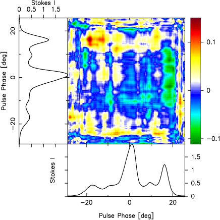
Figure 7: The top plot shows the cross-correlation between components I and delayed V of pulses 800-1944 of the 325-MHz PS. Note the correlation peaks around +94-95 $P_{1}$ of up to 12%, significantly higher than in the adjacent regions; however, no extraordinary correlation is seen at a lag of –53 $P_{1}$. The +94-$P_{1}$ delay longitude-longitude correlation is shown in the lower display, where the correlation between components I and delayed V is evident.

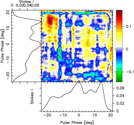
Figure 8: Cross-correlation plots as in Fig. 7 between components I and delayed V of pulses 1-600 of the 610-MHz PS. Again we see a prominent peak at a lag of +97 $P_{1}$, but little at –50 $P_{1}$. The bottom panel shows the longitude-longitude correlation map of the same 610-MHz PS interval in Fig. 3 (bottom) at a delay of +97 $P_{1}$. Here the PS has been smoothed by 5 samples. Note the strong correlation between component I and the delayed component V.

VII. Evidence of a Tertiary Modulation Cycle

We now enquire whether the 7-$P_{1}$ cycle is a part of a longer tertiary modulation cycle as might be expected if the observed modulation were produced by a rotating-subbeam “carousel” as found, in particular, for B0943+10 (DR99, DR01). The long period lrf feature in the 610-MHz PS (Fig. 3, bottom) is suggestive of such a cycle—as are its pair of sidebands. It is interesting to note that such a feature was also found in recent Westerbork observations at both 92 (WSE) and 21 cms (WSE)—but its period there cannot be determined accurately. However, an autocorrelation-function (ACF) analysis of several sections of the the 325-MHz, pulse 800-1944 interval identifies a cycle of similar length. The top panel of Figure 5 gives the result of this analysis done for the outer trailing conal component of the 800-1100 $P_{1}$, where the 7-$P_{1}$ corrugation is prominent as expected. Note the prominent peak at a lag of 147 $P_{1}$, which is close to 20 times $P_{3}$. Indeed, this added positive correlation peak is superposed on the 20th 7-$P_{1}$ corrugation. This peak has an amplitude of about 30%, which is 8 times the expected error in the ACF. It is interesting to note the structure in the 7-$P_{1}$ corrugation, which also has a periodicity of about 147 $P_{1}$. The ACF seems to be consistent with a functional form of the type $\cos(2\pi d/147)\cos(2\pi d/7)$, where $d$ is the delay in units of $P_{1}$. Such orderly variations in the correlation could reflect non-uniform patterns in either the spacing or amplitude of the carousal beamlets. The longitude-longitude correlation at a lag of 147 $P_{1}$ (for a slightly longer PS of 800-1700) is displayed in the lower part of Fig. 5. This sequence exhibits slightly lower (yet significant) correlation in the strong trailing conal component. The ACF analysis of the 610-MHz observation also shows significant correlation at 146 $P_{1}$ with a peak at 147 $P_{1}$ as illustrated in the top panel of Figure 6. Unlike the 325-MHz PS, here significant correlation at 147 $P_{1}$ is seen for both the leading and the trailing components as patches of red along the diagonal in the longitude-longitude correlation map (bottom display).

If this 147-$P_{1}$ peak is indicative of the tertiary modulation, which might be produced by a subbeam carousel system, then we might expect that there should be appreciable correlation between components I and V at some part of the 147-$P_{1}$ cycle, reflecting the circumstance that the ‘beamlets’ rotate around the outer cone. Consideration of the emission geometry (see §III and Fig. 9 below) suggests that this interval should be a about 1/3 of the cycle. In both the 325-MHz (pulses 800-1944) and 610-MHz PSs (over pulses 1-600; see Fig. 3 bottom), we find significant cross-correlation between comp. I and delayed comp. V at lags of 94-95 and 96-97 $P_{1}$, respectively, as shown in Figs. 7 and 8. We find no extraordinary cross-correlation between comp. V and delayed comp. I, which we had expected at lags of 53-54 $P_{1}$ at 325 MHz (see Fig. 7) and 50-51 $P_{1}$ at 610 MHz (if we assume the exact circulation time is 147-$P_{1}$). This might result if the actual peak lag fall between two integers. These various correlations reiterate that the carousel ‘beamlets’ rotate positively with longitude.

Finally, the bugaboo question is whether these responses can be aliased, and the answer surely is yes, but it is also very unlikely that they are aliases of higher frequency responses. Were the primary 7-$P_{1}$ modulation a first-order alias, its true frequency would be 0.86 c/$P_{1}$ and period correspondingly 1.16 $P_{1}$. Such a modulation would have to be very very stable to correlate in the manner we find in Fig. 5, and the 147-$P_{1}$ peak would be indicative of 126 beamlets! We thus appear safe in proceeding on the assumption that the 7- and 147-$P_{1}$ features are not aliased.

VIII. Carousel Configuration

We are now in a position to compute polar maps corresponding to the subpulse-modulation patterns discussed above. A carousel circulation time ${\mathaccent 94{P}}_{3}$ of around 147 $P_{1}$ was indicated both directly by the low frequency feature and by ACFs of the PSs (Fig. 5). This, together with the 7-$P_{1}$ $P_{3}$ feature, strongly suggests a carousel with 20 beamlets. We argued above that it is highly unlikely that the features are aliased, and longitude-longitude correlations appear to confirm that the carousel rotates positively with longitude through the outer conal components. The longitude of the magnetic axis is taken at the midpoint between the outer conal component pair, the putative longitude origin used in most of the figures above. And while we have not been able to determine $\alpha$ and $\beta$ more accurately, the “working” values of 25 and +1.8° are sufficiently accurate for our present purposes—the latter implying an “outside” or poleward traverse of the sightline.

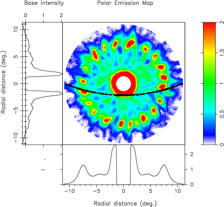
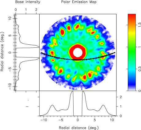
Figure 9: Polar maps constructed using the the respective pulse 1101-1545 (top) and 1-588 (bottom) PSs. Note the roughly regular pattern of 20 ‘beamlets’ in the top map and the irregular pattern in the lower one. The magnetic axis is at the centre of the diagram and the “closer” rotational axis is upward, such that the sightline track sweeps through the pattern as indicated. Here the star rotates counterclockwise, causing the sightline to cut the clockwise-rotating subbeam pattern from right to left; see DR01 for further details. The side panels give the “base” function (which has not been subtracted from the maps here), and the lower panels show the radial form of the average beam pattern.

Figure 9 displays carousel maps for two sections of the 325-MHz PS. Both use a local value of ${\mathaccent 94{P}}_{3}$, computed as 20 times the $P_{3}$ determined within the same interval (7.42 and 7.21 $P_{1}$, respectively). The upper carousel map shows the average pattern of three rotations during a relatively stable interval (pulses 1101-1545; see Fig. 3, top left); whereas the bottom map depicts the average configuration during a less ordered four-${\mathaccent 94{P}}_{3}$ segment (#1-588; see Fig. 3, right). There is a good deal to see in these diagrams. First, there is substantial irregularity even in the upper map, such that 10 regularly spaced beamlets are only seen over half the map. In the lower map, some beamlets have an azimuthal spacing near (360°/20=) 18°, but many do not, so that the broad primary modulation feature in the latter figure is not surprising. Second, the diagrams show virtually no correspondence between the beamlet patterns in the inner and outer conal rings, as expected from our earlier lrf analyses.

IX. Summary and Conclusions

Five-component, core/double-cone pulsars are relatively rare in the normal pulsar population (e.g., Rankin 1993). B1237+25 (e.g., Srostlik & Rankin 2005) is by far the best studied example, and B1857–26 has frequently been compared to it almost as a twin. For the latter, however, little beyond average-profile studies have been available until very recently, and the present study provides the first sensitive PS analysis.

Like B1237+25, B1857–26 exhibits both strong, regular subpulse modulation and null pulses. In the latter, the $P_{3}$ is longer, about 7.4 $P_{1}$ and is confined to the outer conal components. Our two observations have so far identified only one behaviour, or profile mode, as against several in B1237+25. The null fraction is also larger in B1857–26, about 20%$\pm$3%, and twice the value of 10%$\pm$2.5% reported by Ritchings (1976). And also like the former, the nulls in this pulsar are short, typically one pulse and no more than 4 pulses in our observations. Possibly, these are in fact pseudo nulls [as in e.g., B0834+06 (Rankin & Wright 2007a) and B1133+16 (Herfindal & Rankin 2007)] because the maximum null length is about $P_{3}/2$—and thus they represent “empty” sightline traverses through the subbeam carousel system. If so, the 4-$P_{1}$ nulls may occur preferentially in orderly or disorderly intervals of the observations.

Analyses of B1857–26 (unlike B1237+25) provide evidence of a tertiary modulation period ${\mathaccent 94{P}}_{3}$ of some 147 $P_{1}$ at both 325 and 610 MHz. Indications of this tertiary period were first identified via an ACF analysis (e.g., Fig. 5) and then corroborated by a low frequency lrf feature (Fig. 3, bottom). While the ${\mathaccent 94{P}}_{3}$ appears to vary in a range around 146 to 148 $P_{1}$ (just as measured values of $P_{3}$ vary between about 7.3-7.4 $P_{1}$), we have found that in any given interval the circulation time remains 20 times the primary modulation period. Numerically, then, some 20 beamlets would then nominally comprise the carousel pattern, and the more or less regular (or irregular) intervals in our PSs appear to reflect differences in the constancy of spacing and possibly number of beamlets at a given time.

The 147 $P_{1}$ circulation time is again very much larger than the value predicted by the R&S (1975) theory. For B1857–26, with a 612-ms $P_{1}$ and a $B$ of 3$\times$10¹¹ G, this theory predicts only 5.6 $P_{1}$. If ${\bf E}$$\times$${\bf B}$ forces drive the circulation, then it may be that they operate over a larger height range than envisioned in the above theory, as suggested, e.g., by Hibschman & Arons (2001a,b) and Harding et al (2002). Alternatively, a vaccum gap partially screened by thermionic ion flow in the inner acceleration region above the polar cap has been considered (Gil et al 2003) to explain the observed slow drift rates in pulsars.

The PA traverse of B1857–26 presents an interesting case for further analysis. If it is assumed that most of the star’s emission stems from a single OPM, then the PA traverse exceeds 180° by an significant angle. Alternatively, a different mode may predominate on the leading and trailing sides of the profile, or conceivably, the core emission may not follow the RVM. The overall symmetry of the profile, however, does not necessarily support a change in the dominant OPM, as we know of no other good example of a pulsar with such a marked OPM asymmetry about the profile centre. Such asymmetry is sometimes seen in profiles that represent an oblique sightline traverse, but we know of no well vetted example of such asymmetry where the sightline cuts the beam pattern centrally.

Finally, the central core component of PSR B1857–26 provided us little basis for further analysis. Its shape is not at all Gaussian, but otherwise it appears rather steady in both intensity and polarization, showing none of the effects exhibited by B0329+54 (Mitra et al 2007).

References

- Asgekar & Deshpande (2005) Asgekar, A., & Deshpande, A. A. 2005, M.N.R.A.S., 357, 1105
- Backer (1976) Backer D. C. 1976, Ap.J., 209, 895
- Barnard & Arons (1986) Barnard, J. J. & Arons, J. 1986, Ap.J., 302, 138
- Blaskiewicz, Cordes & Wassermann (1991) Blaskiewcz, M., Cordes, J. M., & Wassermann, I. 1991 Ap.J., 370 643.
- Deshpande & Rankin (1999) Deshpande, A. A. & Rankin, J.M. 1999, Ap.J., 524, 1008
- Deshpande & Rankin (2001) Deshpande, A. A. & Rankin, J. M. 2001, M.N.R.A.S., 322, 438
- Everett & Weisberg (2001) Everett, J. E., & Weisberg, J. M. 2001, Ap.J., 553, 341.
- Gil et al (2003) Gil, J., Melikidze, G. I. & Geppert, U., 2003, A&A, 407, 315 M.N.R.A.S., 301, 253.
- Gould & Lyne (1998) Gould, D. M., & Lyne, A. G. 1998, M.N.R.A.S., 301, 253.
- Gupta et al (2004) Gupta, Y., Gil, J., Kijak, J., & Sendyk, M. 2004, M.N.R.A.S., 426, 229.
- Hamilton et al (1977) Hamilton, P. A., McCulloch, P. M., Ables, J. G., & Komesaroff. M. M. 1977, M.N.R.A.S.,180, 1
- Harding et al (2002) Harding, A., Muslimov, A., & Zhang, B. 2002, Ap.J., 576, 366.
- Herfindal & Rankin (2007) Herfindal, J. L. & Rankin, J. M. 2007, M.N.R.A.S., 380, 430
- Hibschman & Arons (2001a) Hibschman, J. A., & Arons, J., 2001a, Ap.J., 554, 624.
- Hibschman & Arons (2001b) Hibschman, J.A., & Arons, J., 2001b, Ap.J., 560, 871.
- Hobbs et al (2005) Hobbs, G., Lorimer, D. R., Lyne, A. G., & Kramer, M. 2005, M.N.R.A.S., 360, 974
- Johnston et al (2005) Johnston, S., Hobbs, G., Vigeland, S., Kramer, M., Weisberg, J. M., & Lyne, A. G. 2005, M.N.R.A.S., 364, 1397
- Komesaroff (1970) Komesaroff, M. M. 1970, Nature, 225, 612
- van Leeuwen et al (1988) van Leeuwen, A.G.J., Stappers, B. W., Ramachandran, R., & Rankin, J. M. 2003, M.N.R.A.S., 399, 223
- Lyne & Manchester (1988) Lyne, A. G., & Manchester, R. N. 1988, M.N.R.A.S., 234, 477
- Manchester et al (1980) Manchester, R. N., Hamilton, P. A., & McCulloch, P. M. 1980, M.N.R.A.S.,192, 153
- McCulloch et al (1978) McCulloch, P. M., Hamilton, P. A., Manchester, R. N., & Ables, J. G. 1978, M.N.R.A.S.,183, 645
- Mitra & Deshpande (1999) Mitra, D., & Deshpande, A. A. 1999, A&A, 346, 906
- Mitra et al (2005) Mitra, D, Gupta, Y. & Kudale, S., 2005, “Polarization Calibration of the Phased Array Mode of the GMRT”, URSI GA 2005, Commission J03a
- Mitra, Rankin & Gupta (2007) Mitra, D., Rankin, J. M. & Gupta, Y. 2007, M.N.R.A.S., 379, 932
- Morris et al (1979) Morris, D., Graham, D. A., Sieber, W., Jones, B. B., Seiradakis, J. H., & Thomasson, P. 1979, A&A, 73, 46
- van Ommen et al (1997) van Ommen, T. D., D’Alessandro, F., Hamilton, P. A., & McCulloch, P. M. 1997, M.N.R.A.S., 287, 307
- Radhakrishnan & Cooke (1969) Radhakrishnan, V., & Cooke, D. J. 1969, Ap. Lett, 3, 225
- Radhakrishnan & Rankin (1993) Radhakrishnan, V., & Rankin, J. M.. 1990, Ap.J., 352, 258.
- Rankin (1983) Rankin J. M. 1983a, Ap.J., 274 333
- Rankin (1983) Rankin J. M. 1983b, Ap.J., 274 359
- Rankin (1986) Rankin J. M. 1986, Ap.J., 301, 901
- Rankin (1993) Rankin J. M. 1993, Ap.J., 405, 285 and Ap.J. Suppl., 85, 145
- Rankin (2007) Rankin J. M. 2007, Ap.J., 664, 443 (20 July 2007)
- Rankin & Ramachandran (2003) Rankin J. M., Ramachandran R. 2003, Ap.J., 590, 411
- Rankin & Wright (2007a) Rankin, J. M. & Wright, G.A.E. 2007a, M.N.R.A.S., 379, 507
- Rankin & Wright (2007b) Rankin, J. M. & Wright, G.A.E. 2007b, M.N.R.A.S., submitted
- Ritchings (1976) Ritchings, R.T. 1976, M.N.R.A.S., 176, 249
- Ruderman & Sutherland (1975) Ruderman, M. A., Sutherland, P. G., 1975, Ap.J., 196, 51
- Srostlik & Rankin (2005) Srostlik, Z., & Rankin, J. M., 2005, M.N.R.A.S., 362, 1121
- Vaughan & Large (1970) Vaughan, A. E. & Large, M. I. 1970, Nature, 225, 167
- Weltevrede et al (2006) Weltevrede, P., Edwards, R., & Stappers, B., 2006, A&A, 445, 243.
- Weltevrede et al (2007) Weltevrede, P., Stappers, B., & Edwards, R., 2007, A&A, 469, 607.