Hierarchical Regular Small-World Networks

Abstract

Two new networks are introduced that resemble small-world properties. These networks are recursively constructed but retain a fixed, regular degree. They possess a unique one-dimensional lattice backbone overlayed by a hierarchical sequence of long-distance links, mixing real-space and small-world features. Both networks, one 3-regular and the other 4-regular, lead to distinct behaviors, as revealed by renormalization group studies. The 3-regular network is planar, has a diameter growing as $\sqrt{N}$ with system size $N$, and leads to super-diffusion with an exact, anomalous exponent $d_{w}=1.306\ldots$, but possesses only a trivial fixed point $T_{c}=0$ for the Ising ferromagnet. In turn, the 4-regular network is non-planar, has a diameter growing as $\sim 2^{\sqrt{\log_{2}N^{2}}}$, exhibits “ballistic” diffusion ($d_{w}=1$), and a non-trivial ferromagnetic transition, $T_{c}>0$. It suggest that the 3-regular network is still quite “geometric”, while the 4-regular network qualifies as a true small world with mean-field properties. As an engineering application we discuss synchronization of processors on these networks.

The description of the “6-degrees-of-separation” phenomenon in terms of small-world (SW) networks by Watts and Strogatz [1] has captured the imagination of many researchers, and was particularly timely as we suddenly found ourselves in a networked world [2, 3, 4]. Such a rich environment requires a diverse set of tools and models for their understanding. Statistical physics, with its notion of universality, provides powerful methods for the classification of complex systems, like the renormalization group (RG) [5, 6, 7, 8].

Figure 1: Display of the 3-regular network HN3 (left) and 4-regular network HN4 (right). HN3 is planar but HN4 is not.

Here, we introduce and study a set of graphs which reproduce the behavior of SW networks without the usual disorder inherent in natural networks. Instead, they attain these properties in a recursive, hierarchical manner that is conducive for RG. The motivation is comparable to regular scale-free networks proposed in Refs. [9, 10] or the Migdal-Kadanoff RG [11, 12, 13]. The benefit of these features is two-fold: For one, we expect that many SW phenomena can be studied analytically on these networks, and that they will prove as useful as, say, Migdal-Kadanoff RG has been for physical systems in low dimensions. Furthermore, possessing such well-understood and regular networks is a tremendous advantage for engineering applications, as it is difficult to manufacture realizations of random networks reliably when we can ascertain their behavior only in the ensemble average. Here, we introduce these networks by discussing their geometry and physical processes on them, such as diffusion, phase transitions, and synchronization.

Each network possesses a geometric backbone, a one-dimensional line of $N=2^{k}$ sites, either open or closed into a ring. To obtain a SW hierarchy, we parameterize

$$n = 2^{i}\left(2j+1\right)$$ (1)

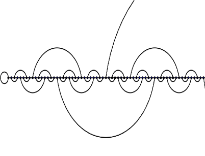
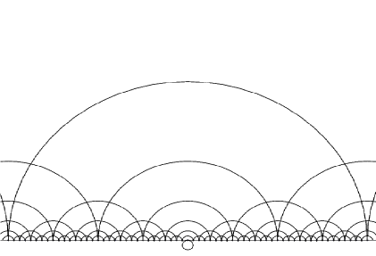
uniquely for any integer $n\not=0$, where $j=0,\pm 1,\pm 2,\ldots$ labels consecutive sites within each level $i\geq 0$ of the hierarchy. For instance, $i=0$ refers to all odd integers, $i=1$ to all integers once divisible by 2 (i.e., $\pm 2,\pm 6,\pm 10,\dots$), and so on. In these networks, both depicted in Fig. 1, in addition to its nearest neighbor in the backbone, each site is also connected with (one or both) of its neighbors within the hierarchy. For example, we obtain a hierarchical 3-regular network HN3 by connecting first neighbors in the 1D-backbone, then 1 to 3, 5 to 7, 9 to 11, etc, for $i=0$, next 2 to 6, 10 to 14, etc, for $i=1$, and 4 to 12, 20 to 28, etc, for $i=2$, and so on. The 4-regular network HN4 is obtained in the same manner, but connecting to both neighbors in the hierarchy. For HN4 it is clearly preferable to extend the line to $-\infty<n<\infty$ and also connect -1 to 1, -2 to 2, etc, as well as all negative integers in the above pattern. These networks resemble models of ultra-diffusion [14, 15], but with inhibiting barriers replaced by short-cuts here.

It is simple to determine geometric properties. For instance, both networks have a clustering coefficient [2] of $1/4$. Next, we consider the diameter $d$, the longest of the shortest paths between any two sites, here the end-to-end distance. Using system sizes $N_{k}=2^{k}$, $k=2,4,6,\ldots$, for HN3, the diameter-path looks like a Koch curve, see Fig. 2. The length $d_{k}$ of each marked path is given by $d_{k+2}=2d_{k}+1$ for $N_{k+2}=4N_{k},$ hence

$$d\sim\sqrt{N}.$$ (2)

This property is reminiscent of a square-lattice of $N$ sites, whose diameter (=diagonal) is also $\sim\sqrt{N}$. HN3 is thus far from true SW behavior where $d\sim\ln N$.

Figure 2: (Color Online) Sequence of shortest end-to-end paths (=diameter, thick lines) for HN3 of size $N=2^{k}$, $k=2,4,8$. Whenever the system size $N$ increases by a factor of 4, the diameter $d$ increases by a factor of $\sim 2$, leading to Eq. (2).

The geometry of HN4 is more subtle. We consider again the shortest path between the origin $n=0$ and the end $n=N=2^{k}$. Due to degeneracies at each level, one has to probe many levels in the hierarchy to discern a pattern. In fact, any pattern evolves for an increasing number of levels before it gets taken over by a new one, with two patterns creating degeneracies at the crossover. We find that the paths here do not search out the longest possible jump, as in Fig. 2. Instead, the paths reach quickly to some intermediate level and follow consecutive jumps at that level before trailing off in the end. This is a key distinguishing feature between HN3 and HN4: Once a level is reached in HN4, the entire network can be traversed at that level, while in HN3 one must switch to lower levels to progress, see Fig. 1.

We derive a recursion equation [16] with the solution

$$d \sim\frac{1}{2} \sqrt{\log_{2}N^{2}}\,\,2^{\sqrt{\log_{2}N^{2}}}\qquad\left(N\to\infty\right)$$ (3)

for the diameter of HN4. Expecting the diameter of a small world to scale as $d\sim\log N$, we rewrite Eq. (3):

$$d_{k} \sim \left(\log_{2}N\right)^{\alpha}\quad{\rm with}\quad\alpha\sim\frac{\sqrt{\log_{2}N^{2}}}{\log_{2}\log_{2}N^{2}}+\frac{1}{2}.$$ (4)

Technically, $\alpha$ diverges with $N$ and the diameter grows faster than any power of $\log_{2}N$ [but less than any power of $N$, unlike Eq. (2)]. In reality, though, $\alpha$ varies only very slowly with $N$, ranging merely from $\alpha\approx 1.44$ to $\approx 1.84$ over nine orders of magnitude, $N=10-10^{10}$.

As a demonstration of the rich dynamics facilitated by these networks, we have modeled diffusion on HN3 and HN4. Starting a random walks at $n=0$, we focus here only on the mean displacement with time,

$$\left\langle\left|n\right|\right\rangle\sim t^{1/d_{w}}.$$ (5)

All walks are controlled by the probability $p$ of a walker to step off the lattice into the direction of a long-range jump. In particular, the walker always jumps either to the left or right neighbor with probability $\left(1-p\right)/2$, but makes a long-range jump with probability $p$ on HN3, or $p/2$ to either the left or right on HN4. In both cases, a simple 1D nearest-neighbor walk results for $p=0$ with $d_{w}=2$ for ordinary diffusion. For any probability $p>0$, long-range links will dominate the asymptotic behavior, and the leading scaling behavior becomes independent of $p$.

Figure 3: Rescaled plot of the mean distance $\left\langle\left|n\right|\right\rangle$ in HN4 for walks up to $t=10^{6}$. We demonstrate that $d_{w}=1$ but with log-corrections by rewriting Eq. (5) as $\left\langle\left|n\right|\right\rangle/t\sim V\left[\ln t\right]^{\beta}$. Then we obtain $\ln\left(\left\langle\left|n\right|\right\rangle/t\right)/\ln\left[\ln t\right]\sim\beta+\ln V/\ln\left[\ln t\right]$ and linearly extrapolate (dashed lines) $1/\ln\left[\ln t\right]\to 0$, estimating $\beta\approx-0.18$ at the intercept, independent of $p$. An effective “velocity” $V$ could be extracted from the slope. For any value besides $d_{w}=1$, these extrapolations would not converge.

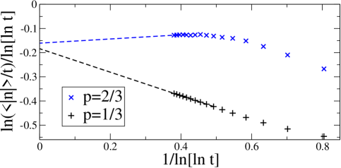
Adapting the RG for random walks in Refs. [17, 18], we find exact results for HN3. The local analysis[19] of the physical fixed point is singular, with a boundary layer instead of a Taylor expansion, yielding an anomalous exponent of $d_{w}=2-\log_{2}\left(\phi\right)=1.3057581\ldots$, containing the (irrational) “golden section” $\phi=\left(1+\sqrt{5}\right)/2$. This is a remarkable exponent also because it is a rare example of a simple walk with super-diffusive ($1<d_{w}<2$) behavior without Levy flights [20, 21, 22], and it would be consistent with experiments leading to super-diffusion [23]. We have not been able to extend this RG calculation to obtain analytic results for HN4 yet, although the high degree of symmetry inherent in these networks (and the simple result obtained) suggest the possibility. For HN4, an annealed approximation and simulations, evolving some $2\times 10^{7}$ walks for $10^{6}$ time steps each, suggest a value of $d_{w}=1$, see Fig. 3. Hence, a walk on HN4 proceeds effectively ballistic, but hardly with linear motion: widely fluctuating jumps conspire just so that a single walker extends outward with an on-average constant velocity in both directions, yet the walk remains recurrent. Clearly, it is easier to traverse HN4 than HN3 because of the above-stated fact that on HN4 a walker can progress repeatedly within a hierarchical level.

We have also studied Ising spin models on HN3 and HN4, with RG and with Monte Carlo simulations. First, we consider the RG for the Ising model on HN3. In this case, all steps can be done exactly but the result turns out to be trivial (for uniform bonds) in the sense that there are no finite-temperature fixed points of the RG flow. Yet, the calculation is instructive, highlighting the large number of statistical models that can be accessed through the hierarchical nature of the process, and it is almost identical in outcome to the treatment below for HN4. That small difference is just enough to provide HN4 with a non-trivial $T_{c}>0$, which we confirm numerically.

Figure 4: Depiction of (exact) RG step for the Ising model on HN3. Tracing out odd-labeled variables $x_{n\pm 1}$ for all $n=2(2j+1)$, in the left plot leads to the renormalized couplings $(L^{\prime},K^{\prime}_{0},K^{\prime}_{1})$ on the right in terms of the old couplings $(L,K_{0},K_{1})$. Unlabeled bonds correspond to $K_{i\geq 2}$. HN3 does not contain couplings of type $(L,L^{\prime})$, but they become relevant during the RG process. Random walks on HN3 lead to a topologically equivalent, but more involved RG step [19].

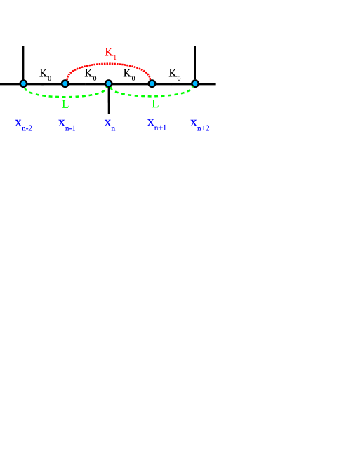
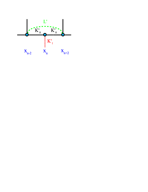
The RG consists of recursively tracing out odd-relabeled spins $x_{n\pm 1}$, see Fig. 4. The $x_{n\pm 1}$ are connected to their even-labeled nearest neighbors on the lattice backbone by a coupling $K_{0}$. At any level, each $x_{n\pm 1}$ is also connected to one other such spin $x_{n\mp 1}$ across an even-labeled spin $x_{n}$ with $n=2\left(2j+1\right)$ in Eq. (1) that is exactly once divisible by 2. Let us call that coupling $K_{1}$, all other couplings are $K_{i>1}$. During the RG process, a new coupling $L$ (dashed line in Fig. 4) between next-nearest even-labeled neighbors emerges. Putting all higher level terms into $\mathcal{R}$, we can section the Hamiltonian

$$-\beta\mathcal{H} = \sum_{\left\{n=2(2j+1)\right\}}\left(-\beta\mathcal{H}_{n}\right)+\mathcal{R}\left(K_{2},K_{3},\ldots\right),$$ (6)

where each sectional Hamiltonian is given by

$$-\beta\mathcal{H}_{n}=\sum_{m=n-2}^{n+1}K_{0}x_{m}x_{m+1}+K_{1}x_{n-1}x_{n+1}+L\left(x_{n-2}x_{n}+x_{n}x_{n+2}\right)$$

with $\left(K_{0},K_{1},L\right)$ as unrenormalized couplings and we neglected an overall energy scale. After tracing out the odd-labeled spins in each $\exp\left[-\beta\mathcal{H}_{n}\right]$, we identify the renormalized couplings (neglecting $I^{\prime}$):

$$K^{\prime}_{0} = L+\frac{1}{2}\ln\cosh\left(2K_{0}\right)+\frac{1}{4}\ln\left[1+\tanh\left(K_{1}\right)\tanh^{2}\left(2K_{0}\right)\right],$$

$$L^{\prime} = \frac{1}{4}\ln\left[1+\tanh\left(K_{1}\right)\tanh^{2}\left(2K_{0}\right)\right],$$ (7)

and $K^{\prime}_{i}=K_{i+1}$ f. a. $i\geq 1$. The high-$T$ solution $K_{0}^{*}=L^{*}=0$ is a trivial fixed point of Eq. (7). Excluding that and eliminating $L^{*}$ yields $1=\tanh\left(K_{1}\right)\tanh\left(2K_{0}^{*}\right)$, which has only the $T_{c}=0$ solution $K_{0}^{*}=\infty$ (where also $K_{1}=J_{1}/T\to\infty$). Note, however, that the RG recursions (7) have a remarkable property due to the hierarchical structure of the network: The next-level coupling $K_{1}$ appears as a free parameter and acts as “source term” that could be chosen to represent physically interesting situations, e. g. disorder or distance-dependence. For instance, with $K_{i}$ as an increase function of distance $r_{i}=2^{i+1}$, a non-trivial fixed point could be created.

In contrast, HN4 provides a non-trivial solution for the Ising model even for uniform bonds, as expected for a mean-field system. Again, an exact result for HN4 is elusive, although in light of the inherent symmetries such a solution appears possible. Instead, we proceed to a Niemeijer-van Leeuwen cumulant expansion [7] and compare with our numerical simulations. The Hamiltonian indeed has an elegant hierarchical form separating the lattice backbone and long-range couplings:

$$-\beta\mathcal{H}=\sum_{n=1}^{2^{k}}K_{0}x_{n-1}x_{n}+\sum_{i=1}^{k}\sum_{j=1}^{2^{k-i}}K_{i}x_{2^{i-1}\left(2j-1\right)}x_{2^{i-1}\left(2j+1\right)}.$$ (8)

For the RG, we set $-\beta\mathcal{H}=-\beta\mathcal{H}_{0}-\beta\mathcal{V}+\mathcal{R}$ with

$$-\beta\mathcal{H}_{0} = \sum_{j=1}^{2^{k-1}}K_{0}x_{2j-1}\left(x_{2j-2}+x_{2j}\right)+\sum_{j=1}^{2^{k-1}}Lx_{2j-2}x_{2j},$$

$$-\beta\mathcal{V} = \sum_{j=1}^{2^{k-1}}K_{1}x_{2j-1}x_{2j+1},$$ (9)

adding new couplings $L$ that emerge during RG, as in Fig. 4. Tracing out odd spins and relabeling all remaining even spin variables $x_{n}\to x^{\prime}_{n/2}$, the cumulant expansion applied to Eq. (9) yields a new Hamiltonian $-\beta\mathcal{H}^{\prime}$, formally identical to Eq. (8), with the rescaled couplings

$$K^{\prime}_{0} = L+\frac{1}{2}\ln\cosh\left(2K_{0}\right)+\frac{K_{1}}{2}\tanh^{2}\left(2K_{0}\right),$$ (10)

$$K^{\prime}_{1} = K_{2}+\frac{K_{1}}{4}\tanh^{2}\left(2K_{0}\right),\quad L^{\prime}=\frac{K_{1}}{4}\tanh^{2}\left(2K_{0}\right).$$

and $K^{\prime}_{i}=K_{i+1}$ for $(i\geq 2)$. These are the same relation one would obtain for the 1D-Ising model with nnn couplings, if $K_{1}\equiv L$ and $K_{i}=0$ for $i\geq 2$. In that case, one would find – correctly – that there are no non-trivial fixed points. The $K_{2}-$term, which appears as an arbitrary source again at every RG step, if chosen appropriately, provides the sole ingredient for a non-trivial outcome. But unlike for HN3, here already uniform ($i$-independent) $K_{i}$ obtain $T_{c}>0$. Holding the source terms fixed, $K_{i\geq 2}\equiv 1$, we find a single nontrivial fixed point at $K_{0}^{*}\approx 0.2781$, $K_{1}^{*}\approx 1.0681$, $L^{*}\approx 0.0681$. An analysis of the RG flow [7] in Eqs. (Hierarchical Regular Small-World Networks), starting with identical $K_{i}\equiv\beta J$ f. a. $i$, yields $T_{c}\approx 2.2545J$. Simulations on HN4 with uniform bonds for increasing system sizes $N=2^{k}$ accumulate to $T_{c}=2.1(1)J$.

Figure 5: Width $\left<w^{2}\right>$ as a function of $N$. The 1D-loop without long-range connections diverges most strongly, linear in $N$, while the random one-per-node SW connections keep the width finite. The width diverges with a weak power of $N$ for HN3, but merely logarithmically for HN4.

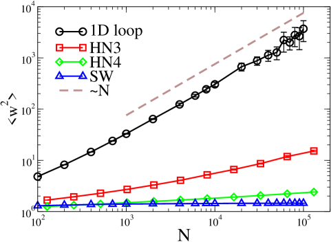
Finally, we demonstrate the usefulness of having a regular (i.e., non-random) network at hand with fixed, predictable properties. Synchronization is a fundamental problem in natural and artificially coupled multicomponent systems [24]. Since the introduction of SW networks [1], it has been established that such networks can facilitate autonomous synchronization [25, 26]. In a particular synchronization problem the nodes are assumed to be task processing units, such as computers or manufacturing devices. Let $h_{i}(t)$ be the total task completed by node $i$ at time $t$ and the set $\{h_{i}(t)\}_{i=1}^{N}$ constitutes the task-completion (synchronization) landscape, where $N$ is the number of nodes. In this model the nodes whose tasks are smaller than those of their neighbors are incremented by an exponentially distributed random amount, i.e., the node $i$ is incremented, if $h_{i}(t)\leq\min_{j\in S_{i}}\{h_{j}(t)\}$, where $S_{i}$ is the set of nodes connected to node $i$; otherwise, it idles. In its simplest form the evolution equation is $h_{i}(t+1)=h_{i}(t)+\eta_{i}(t)\prod_{j\in S_{i}}\Theta\left(h_{j}(t)-h_{i}(t)\right)$, with iid random variables of unit mean, $\eta_{i}(t)$, $\delta$-correlated in space and time, and $\Theta$ as the Heaviside step function.

The average steady-state spread or width of the synchronization landscape (degree of de-synchronization) can be written as $w^{2}=(1/N)\sum_{i=1}^{N}(h_{i}-\bar{h})^{2}$ [26]. In low dimensional regular lattices the synchronization landscape belongs to the Kardar-Parisi-Zhang [27] universality class, a rough desynchronized state dominated by large-amplitude long-wavelength fluctuations, where width diverges with $N$. On the contrary, the width becomes finite [26] on a SW model in which each node is connected to nearest neighbors and one random neighbor. In Fig. 5, we show the width as a function of $N$ for a 1D loop and SW, as well as HN3 and HN4. The width for HN4 behaves very similar to SW, with at most a logarithmic divergence in $N$, while it diverges with power-law for HN3, but weaker than for a 1D-loop. HN4, thus, provides very similar properties to SW with the benefit of a regular and reproducible structure that is easy to manufacture, and that is potentially analytically tractable.

In conclusion, we introduced a new set of hierarchical networks with regular, small world properties and demonstrated their usefulness for theory and engineering applications with a few examples. Aside from the countless number of statistical models that can be explored with RG on these networks, they also provide a systematic way to interpolate off a purely geometric lattice into the SW domain, possibly all the way into the mean-field regime (for HN4). Even though at this point complete solutions on HN4 elude the authors, even the leading approximation provides significant insight.

B.G. was supported by the NSF through grant #0312510 and H.G. was supported by the U.S. DOE through DEAC52-06NA25396.

References

- [1] D. J. Watts and S. H. Strogatz. Collective dynamics of ’small-world’ networks. Nature, 393:440–442, 1998.
- [2] S. Boccaletti, V. Latora, Y. Moreno, M. Chavez, and D.-U. Hwang. Complex networks: Structure and dynamics. Phys. Rep., 424:175, 2006.
- [3] Albert-Laszlo Barabasi. Linked: How Everything Is Connected to Everything Else and What It Means for Business, Science, and Everyday Life. Plume Books, April 2003.
- [4] M. E. J. Newman, S. H. Strogatz, and D. J. Watts. Random graphs with arbitrary degree distributions and their applications. Phys. Rev. E, 64(2):026118, Jul 2001.
- [5] N. Goldenfeld. Lectures on Phase Transitions and the Renormalization Group. Addison-Wesley, Reading, 1992.
- [6] H. Eugene Stanley. Scaling, universality, and renormalization: Three pillars of modern critical phenomena. Rev. Mod. Phys., 71(2):S358–S366, Mar 1999.
- [7] M. Plischke and B. Bergersen. Equilibrium Statistical Physics, 2nd edition. World Scientifc, Singapore, 1994.
- [8] M. E. J. Newman and D. J. Watts. Renormalization group analysis of the small-world network model. Physics Letters A, 263:341–346, 1999.
- [9] A.-L. Barabasi, E. Ravasz, and T. Vicsek. Deterministic scale-free networks. Physica A, 299:559–564, 2001.
- [10] J. S. Andrade, H.-J. Herrmann, R. F. S. Andrade, and L. R. da Silva. Apollonian networks: Simultaneously scale-free, small world, euclidean, space filling, and with matching graphs. Phys. Rev. Lett., 94:018702, 2005.
- [11] A. A. Migdal. Recursion relations in gauge field theories. J. Exp. Theo. Phys., 42:743–746, 1976.
- [12] L. P. Kadanoff. Notes on migdal’s recursion formulas. Ann. Phys., 100:359–394, 1976.
- [13] M. Hinczewski and A. N. Berker. Inverted berezinskii-kosterlitz-thouless singularity and high-temperature algebraic order in an ising model on a scale-free hierarchical-lattice small-world network. Phys. Rev. E, 73:066126, 2006.
- [14] B A Huberman and M Kerszberg. Ultradiffusion: the relaxation of hierarchical systems. J. Phys. A: Math. Gen., 18(6):L331–L336, 1985.
- [15] Andrew T. Ogielski and D. L. Stein. Dynamics on ultrametric spaces. Phys. Rev. Lett., 55(15):1634–1637, Oct 1985.
- [16] S. Boettcher, B. Gonçalves, and J. Azaret. Geometry and dynamics for hierarchical regular networks. arXiv:0805.3013.
- [17] B Kahng and S Redner. Scaling of the first-passage time and the survival probability on exact and quasi-exact self-similar structures. J. Phys. A: Math. Gen., 22:887–902, 1989.
- [18] S. Redner. A Guide to First-Passage Processes. Cambridge University Press, Cambridge, 2001.
- [19] S. Boettcher and B. Gonçalves. Anomalous diffusion on the hanoi network. arXiv:0802.2757.
- [20] S. Havlin and D. Ben-Avraham. Diffusion in disordered media. Adv. Phys., 36:695–798, 1987.
- [21] R. Metzler and J. Klafter. The restaurant at the end of the random walk: recent developments in the description of anomalous transport by fractional dynamics. J. Phys. A: Math. Gen., 37:R161–R208, 2004.
- [22] A. Fischer, S. Seeger, K.-H. Hoffmann, C. Essex, and M. Davison. Modeling anomalous superdiffusion. J. Phys. A: Math. Theor., 40:11441–11452, 2007.
- [23] T. H. Solomon, E. R. Weeks, and H. L. Swinney. Observation of anomalous diffusion and l vy flights in a two-dimensional rotating flow. Phys. Rev. Lett., 71:3975 – 3978, 1993.
- [24] S. Strogatz. Exploring complex networks. Nature, 410:268, 2001.
- [25] Mauricio Barahona and Louis M. Pecora. Synchronization in small-world systems. Phys. Rev. Lett., 89(5):054101, Jul 2002.
- [26] G. Korniss, M. A. Novotny, H. Guclu, Z. Toroczkai, and P. A. Rikvold. Suppressing roughness of virtual times in parallel discrete-event simulations. Science, 299:677–679, 2003.
- [27] M. Kardar, G. Parisi, and Y.-C. Zhang. Dynamic scaling of growing interfaces. Phys. Rev. Lett., 56:889–892, 1986.