Parton correlation functions and factorization in deep inelastic scattering

Abstract:

We outline the basic properties of a pertubative QCD factorization formalism that maintains exact over-all kinematics in both the initial and final states. Such a treatment requires the use of non-perturbative factors that depend on all components of parton four-momentum. These objects are referred to as parton correlation functions. We describe the complications faced in defining parton correlation functions and discuss recent progress. Emphasis is placed on the need for precise operator definitions in a complete derivation of factorization.

1 Exact over-all kinematics and the need for a generalized treatment of factorization

The standard collinear factorization theorems of perturbative QCD (pQCD) rely on a number of kinematical approximations that change the momentum of the final state particles. In inclusive deep inelastic scattering (DIS), for example, the struck parton is assumed to have a non-zero component of four-momentum only in the plus direction corresponding to the target beam direction.

It has been known for some time that neglecting the transverse component of the struck parton momentum is not always valid. This has lead to studies of “$k_{t}$-factorization” involving $k_{t}$-unintegrated (or just unintegrated) parton distribution functions [1]. More recently, it has been noted that in certain cases over-all four-momentum conservation (involving both transverse momentum and parton invariant energy) must be enforced to avoid making large errors, particularly when the details of final states are important [2]. This has motivated the formulation of factorization theorems in which no approximation is made on the momenta of initial and final states. The non-perturbative objects in such a factorization formula will depend on all components of parton four-momentum. We call these fully unintegrated objects parton correlation functions (PCFs). In these proceedings we outline the basic structure of the fully unintegrated formalism proposed in [3]. In addition, we re-emphasize the need for exact operator definitions for the non-perturbative factors in a factorization formalism.

2 The role of operator-based definitions

Having non-perturbative factors rooted in operator definitions is important for the derivation of a reliable factorization formula. To understand this, let us briefly review the basic requirements of a factorization theorem:

• For a given process with hard scale $Q$, a factorization formula exists if the cross section can be written approximately as a generalized product of several factors. The hard scattering coefficient $C$ should involve only lines that are off-shell by order $Q$ and can be calculated explicitly in pQCD. The other factors involve infrared and collinear lines and parameterize the non-perturbative physics. Errors should be suppressed by powers of $\Lambda/Q$ where $\Lambda$ is a typical hadronic mass scale.

• The non-perturbative factors must be parameterized by experimental data. But if factorization formulae exist for different processes, and involve the same non-perturbative factors, then one can parameterize a non-perturbative factor in one experiment and use it in another to make first-principle predictions. If this can be shown, we say that the non-perturbative factors are universal.

Operator definitions are what allow for a comparison of the soft and collinear factors used in different processes. Hence, they are needed if one is to have confidence in the second bulleted statement above. As an example, consider the simple case of totally inclusive DIS. The definition of the integrated parton distribution function should arise naturally from the sequence of approximations needed to factorize the hadronic tensor. The hadronic tensor written using standard notation is,

$$W^{\mu\nu}(P,q)=4\pi^{3}\sum_{X}\langle p\left|J^{\mu}(0)\right|X\rangle\langle X\left|J^{\nu}(0)\right|p\rangle\delta^{(4)}(p_{X}-(p+q)).$$ (1)

Starting with this very basic formula and applying certain approximations, one can derive the formula,

$$P_{\mu\nu}W^{\mu\nu}(P,q)=P_{\mu\nu}H^{\mu\nu}_{j}(q,\xi,\mu)\otimes f_{j/h}(\xi,\mu)+\mathcal{O}(\Lambda/Q\left|P_{\mu\nu}W^{\mu\nu}(P,q)\right|),$$ (2)

where $P_{\mu\nu}$ is defined to act on the electromagnetic vertices to project out a particular structure function, say $F_{1}$. The function $f_{j/h}(\xi,\mu)$ is the usual expression for the fully integrated parton distribution function (PDF),

$$f_{j/h}(\xi,\mu)=\int\frac{dw^{-}}{4\pi}e^{-i\xi p^{+}w^{-}}\\ \times\langle p|\bar{\psi}(0,w^{-},{\bf 0}_{T})V^{\dagger}_{w}(u_{\rm J})\gamma^{+}V_{0}(u_{\rm J})\psi(0)|p\rangle.$$ (3)

Here $\psi$ is the quark field operator, and $V_{0}(u_{J})$ is a Wilson line operator in the direction $u_{J}=(0,1,{\bf 0}_{t})$ needed to make the definition exactly gauge invariant. The lowest order hard scattering matrix element is the usual one involving only the electromagnetic vertex. Using it in Eq. (2) reproduces the parton model. Higher order corrections are calculated by considering more complex graphs and applying a sequence of subtractions to remove double counting. The unregulated PDFs contains the usual ultraviolet divergences which are effectively removed using standard renormalization techniques, with a renormalization scale $\mu$. The resulting evolution equations describe the well-known scaling violations of DIS. The fact that the PDF $f_{j/h}(\xi,\mu)$ also appears in the factorization formula for other processes means that it can be parameterized and used for future predictions.

One may hope to have the same powerful structure in a more general unintegrated formalism. In a treatment that includes the transverse momentum of the struck parton, it is tempting to propose a differential definition for the $k_{t}$-unintegrated parton distribution,

$$\mathcal{F}_{j/p}({\bf k}_{t},\xi)\stackrel{{\scriptstyle??}}{{=}}\left.\frac{\partial f_{j/h}(\xi,\mu^{2})}{\partial\ln\mu^{2}}\right|_{\mu^{2}=k_{T}^{2}}.$$ (4)

Studies of small-x physics [1] suggest that this is probably correct to a good approximation in the small-$x$ limit. However, it is unclear in general whether there is a reliable sequence of approximations that allow (4) to be factorized out of the hadronic tensor with only a hard scattering coefficient left over. The universality of the $k_{t}$-dependent PDF is thus called into question.

The situation with $k_{t}$-unintegrated PDFs is further complicated by the fact that the most obvious candidate for a definition is unsuitable for use in factorization. Namely, if we leave one of the integrals in Eq. (3) undone, we obtain the seemingly natural definition,

$$\mathcal{F}_{j/p}(x,{\bf k}_{T},\mu)\stackrel{{\scriptstyle??}}{{=}}\int\frac{dw^{-}d{\bf w}_{T}}{16\pi^{3}}e^{-ixp^{+}w^{-}+i{\bf k}_{T}\cdot{\bf w}_{T}}\\ \times\langle p|\bar{\psi}_{j}(0,w^{-},{\bf w}_{T})V^{\dagger}_{w}(n)\gamma^{+}V_{0}(n)\psi_{j}(0)|p\rangle.$$ (5)

However, this definition acquires divergences from gluons moving with infinite rapidity in the outgoing quark direction making it inappropriate for use as a PDF. (See [4] for a more detailed discussion.) An additional problem, pointed out by Belitsky et al. [5], is that exact gauge invariance requires the insertion of a gauge link at light-cone infinity. Recent work in providing consistent operator definitions for $k_{t}$-unintegrated PDFs has been done by Hautmann and Soper [6].

3 A fully unintegrated formalism

As already mentioned, there are situations where we need a formalism based on non-perturbative objects that depend on all components of parton four-momentum. An approach to factorization using PCFs was formulated in [8] for the case of a scalar field theory, and extended to the case of a gauge theory in [3].. We summarize these results now. To save space we do not list the actual definitions, but rather outline the basic structure of their derivation. For all details, the reader is referred to [3].

To avoid making errors of the type discussed in the first section, one must begin with graphs of the general structure shown in Fig. 1(a) rather than the usual handbag diagram. The bubbles represent sums of diagrams contributing to initial and final states. The extra gluons shown attaching the collinear bubbles to the hard scattering bubble represent possible extra target and final state collinear gluons. In addition, there may be arbitrarily many soft gluons connecting the outgoing jets via a soft bubble. Before factorization, these bubbles are $\Phi$ for the target collinear lines, $\mathcal{J}$ for the jet collinear lines, and $\mathcal{B}$ for the soft lines.

It follows from general arguments [7] that graphs with the topology of Fig. 1(a) are the most general contributions to DIS involving a single outgoing jet. Applying Ward identities to the sum of graphs with this allows the extra soft and collinear gluons to be disentangled into separate factors. After topological factorization is achieved, the graph takes the form shown in Fig. 1(b). The different PCFs include a soft factor $S$, a jet factor $J$, and a target factor(fully unintegrated PDF) $F$. The PCFs are represented graphically by the bubbles. The double lines associated with each bubble are eikonal lines that correspond to Wilson lines in the definitions of the PCFs. To be consistent with factorization, the definitions of the PCFs also require double counting subtractions. (To avoid clutter, the double counting subtractions aren’t shown explicitly in the figure.) The factors S,J, and F can ultimately be shown to arise from operator definitions of the PCFs. Schematically, the final factorization formula is,

$$\sigma=C\otimes F\otimes J\otimes S+\mathcal{O}\left(\left(\Lambda/Q\right)^{a}|\sigma|\right),$$ (6)

where $\sigma$ is a measurable quantity such as a cross section or structure function and $a>0$.

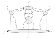
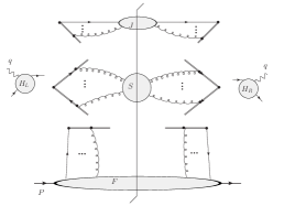
(a)	(b)

Figure 1: (a) General contribution to DIS at lowest order and (b) Structure of the graph after factorization.

4 Outlook

Our factorization formula is now more complicated than the usual one in Eq. (2). Each PCF depends on several parameters and each needs to be fitted to experimental data. For the fully unintegrated formalism to be practical, factorization formulae using the same PCFs will need to be derived for a number of non-trivial processes. In addition to evolution in $\mu$, the evolution equations for the PCFs will also involve evolution in other rapidity variables which act as effective cutoffs on rapidity divergences. One hope is to relate this type of evolution to more common approaches such as the CCFM equation.

As we have mentioned, the factorization formula represented schematically in Fig. 1(b) is only complete at lowest order in the hard scattering coefficient because it involves only one outgoing jet line. However, this result is already quite useful because it now allows higher order corrections to be obtained via double counting subtractions applied to more complicated graphs. As in [8] for the scalar field theory, the hard scattering coefficients are expected to be ordinary functions as opposed to the generalized functions (e.g. $\delta$-functions) that appear in the hard coefficients of the standard integrated formalism.

References

-
[1]
L. N. Lipatov,
Phys. Rept. 286, 131 (1997)
[arXiv:hep-ph/9610276].
M. A. Kimber, A. D. Martin and M. G. Ryskin, Phys. Rev. D 63, 114027 (2001) [arXiv:hep-ph/0101348]. -
[2]
J.C. Collins and H. Jung,
arXiv:hep-ph/0508280.
G. Watt, A.D. Martin, and M.G. Ryskin, Eur. Phys. J. C 31, 73 (2003). - [3] J. C. Collins, T. C. Rogers and A. M. Stasto, arXiv:0708.2833 [hep-ph].
- [4] J. C. Collins, Acta Phys. Polon. B 34, 3103 (2003) [arXiv:hep-ph/0304122].
- [5] A.V. Belitsky, X. Ji and F. Yuan, Nucl. Phys. B 656, 165 (2003).
- [6] F. Hautmann and D. E. Soper, Phys. Rev. D 75, 074020 (2007) [arXiv:hep-ph/0702077].
- [7] S.B. Libby and G. Sterman, Phys. Rev. D 18, 4737 (1978).
- [8] J. C. Collins and X. Zu, JHEP 0503, 059 (2005) [arXiv:hep-ph/0411332].