How to control nonlinear effects in Binder cumulants
Abstract
We point out that ignoring nonlinear effects in finite size scaling may lead to errors in estimates of the critical temperature and Binder cumulants. We show that the order of magnitude of these effects can be estimated from data at relatively small volume. Using this estimate, we propose to use linear fits in increasingly small temperature regions as the volume is increased (rather than using a fixed temperature interval). The choice of the exact coefficient of proportionality can be optimized and reveals interesting crossing patterns among estimates. We show that the new procedure works very well for Dyson’ hierarchical model. We discuss applications of the method for 3 dimensional spin models and finite temperature lattice gauge theories and comment on the nonlinear effects for existing calculations.
pacs:
11.15.-q, 11.15.Ha, 64.60.an, 64.60.De1 Introduction
The study of the Binder cumulants for isolated systems of various sizes has been an important tool to determine the critical temperature and universal quantities of spin models [1, 2, 3, 4, 5, 6, 7, 8, 9] and lattice gauge theory models at finite temperature [10, 11, 12, 13, 14, 15, 16]. The basic idea is that the intersections among Binder cumulants curves for systems of different sizes obey scaling relations often referred to as Finite Size Scaling (FSS).
Linearization in the scaling variables is often used to derive approximate FSS relations for the Binder cumulants and the critical temperature that allow, in principle, simple linear extrapolations to infinite volume [1, 3]. However, in practice, the errors bars on the intersections are often of the same order as the finite size variations and the linearity of the data is not always obvious. Examples of such graphs are figure 7 in [3] or figures 3, 4 and 6 of [16]. For this reason, authors will sometimes prefer to rely on a single intersection for the two largest volumes available that has potentially smaller errors [6, 16].
A possible source of systematic error in these infinite volume extrapolations are the nonlinear terms that have been neglected in the derivation of the linear FSS formulas. If these effects are small enough, it is difficult to disentangle them from the statistical errors. Typically, we are talking about a 1-2 percent effect. This may sound small, however, for the hierarchical sigma models where very accurate calculations can be performed, the differences between the Binder cumulants at successive values of are less than 2 percent for low values of [17]. Consequently, it is reasonable to set accuracy goals of less than 1 percent for the Binder cumulants, especially if the estimate is used to establish that a particular model belongs to a known class of universality.
In this article, we discuss quantitatively the effects of the nonlinear terms in FSS with an example and we propose a new procedure to obtain infinite volume estimates that are minimally distorted by the nonlinear effects. The procedure can be used for spin models or lattice gauge models and is a notation that can be used interchangeably for either the inverse temperature in Ising-like models or in gauge theory.
One purpose of the article is to provide a specific improvement to the common practice of using data at the same, equally spaced, values of for all value of the linear size (we call this the “fixed interval procedure”). Clear examples of the fixed interval procedure can be seen in figure 6 of [2], figure 11 of [4], figure 7 of [10], figure 1 of [11] and figure 1 of [16] where the fourth order cumulant is plotted versus or the temperature. In the large volume limit, the cumulant becomes a function (that we will call ) of the reduced variable , with the usual correlation length exponent. This function can be approached at sufficiently large volume by plotting the cumulant versus this reduced variable. When this is done, the data “collapses” up to some finite size corrections. It seems clear that in order to reduce the nonlinear effects, we should shrink the range of as increases.
This idea seems simple, however its practical implementation is non-trivial. First, we need to estimate the size of the nonlinear effects. Second, we only know with a finite accuracy and the interval cannot be shrunk to a size much smaller than the uncertainties on . We need to find a compromise between two conflicting requirements. On one hand, the interval needs to be small enough to reduce the nonlinear effect. On the other hand, if the interval is too small, we may not cover properly the region where the linear approximation is valid which could result in errors for the intersections. The main technical question that we address here is: can we find an optimal width for the interval were both requirements can be reasonably satisfied? It is difficult to answer this question for the gauge or spin models discussed above because it is hard to extract the nonlinear effects from the statistical errors. In addition, we have no independent estimates of the infinite volume cumulants and calculations at large volume are CPU demanding.
We will address this question in a model where the practical issues mentioned above can be avoided, namely Dyson hierarchical model [18] with an Ising measure. In this model, it possible to block spin very accurately with methods [19, 20, 21] that have been recently reviewed in [22]. This allows us to make very accurate calculations at very large volume (linear size up to sites) that cannot be reached with ordinary Monte Carlo methods. The free parameter of this model has been fixed in such a way that free Gaussian fields scale like in 3 dimensions. The technical details are given in A. These large volume numerical calculations will be used later to check the accuracy of estimates made using data at much smaller volumes (linear size up to 256 sites as in existing Monte Carlo (MC) calculations).
Our presentation is focused on the estimation of the infinite volume critical temperature and the (universal) fourth order Binder cumulant. This quantity is defined precisely in section 2 where we introduce other notations and state the problem. We provide a parametrization of the nonlinear effects for the fourth order cumulant in terms of two new parameters (see equation (2.7)). Accurate numerical values of these parameters are given in A in the case of the hierarchical model. We then discuss the linearization and graphs testing its validity.
The new method that we propose here (the “shrinking interval procedure”) is presented in section 3. It proceeds in two steps. First, we need to estimate the size of the nonlinear effects using data at relatively small volume. We explain that the important quantity is the ratio of the linear to quadratic leading amplitudes (called ). We show in B that this quantity can be estimated with reasonable accuracy using a pencil and a ruler on a graph showing the Binder cumulant versus at relatively small volume. We then propose to use a shrinking range where is an adjustable small parameter which we shall see, can picked in an optimal way by localizing crossings in infinite volume extrapolations.
In section 4 we compare the shrinking interval procedure with the fixed interval procedure. The calculations are done using a number of values of and linear sizes that are typical in existing MC calculations. We emphasize that in doing these calculations, we did not use our prior knowledge of the critical temperature, Binder cumulant or amplitudes given A, however we used our knowledge of the critical exponents and . We first used a fixed value of (0.05) and found much better result than with the fixed interval method. We then compared infinite volume extrapolations for and the cumulant, for different values of . The results are displayed in figure 4 where we see remarkable crossings (among extrapolation curves for different maximal volume) at approximately the same value of for the two quantities. We compared the results for this optimal value with the accurate ones and found relative errors of less than for and of less than for the cumulant.
Figure 4 is the most important result of the paper. It shows that an optimal value of can selected using the numerical results. It is crucial to realize that the crossing means that for the optimal value of , results at not too large volume provide very accurate results. One should also appreciate the number of large volume calculations involved in producing the two graphs that would take a prohibitively long time for 4 dimensional lattice gauge theory.
In section 5, we discuss the effects of the nonlinear terms for the calculations done in the literature and we conclude with possible applications of the new method.
2 Statement of the problem and notations
The new method proposed in this article can be used for two types of models. First, the spin models where denotes the inverse temperature in appropriate units. In the literature on the 3 dimensional Ising model [9] is often denoted . Second, the lattice gauge models with gauge group at finite temperature where is the number of sites in the Euclidean time direction and the lattice spacing. For these models is not the inverse temperature. However, if we use the one-loop scaling [11],
| (2.1) |
This formula illustrates that for the finite temperature gauge model, implies because the ordered phase of these models corresponds to high and high .
In summary, the notation can be used for both types of models with a consistent meaning: the ordered phase corresponds to . For this reason, we will define a reduced (or ) variable:
| (2.2) |
Other choices such as lead to similar linear behavior near but have different nonlinear behavior. These considerations are important if we want to connect with other expansions [23, 24].
We now consider finite size scaling for isolated blocks in 3 dimensions. The spin models are defined on symmetric cubic lattice sites. The gauge models are defined lattices. We use the convention for the variable number of sites (while is kept fixed) in order to have unified notations. In both cases, the system is not in contact with a larger system but isolated and defined with suitable boundary conditions.
Under a RG transformation where the lattice spacing , we have and , where the are the nonlinear scaling variables which transform multiplicatively. We denote the only relevant scaling variable (we will not deal with external fields) and we will only consider the effect of the first irrelevant variable denoted . We assume that the exponents , are known with good precision as it is the case when we are testing the hypothesis that a particular system belongs to a well studied class of universality. In addition, we assume the expansions
| (2.3) | |||||
| (2.4) |
We define the fourth Binder cumulant as
| (2.5) |
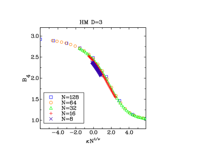
with the average of the order variable (spin for Ising, Polyakov’s loop in the time direction for gauge theory) in 3 dimensions. Directly related quantities appear in the literature such as or etc. Due to the lack of consensus, we have picked a form that has limits that are easy to remember. Both numerator and denominator are unsubtracted averages and so this quantity can be calculated at large volume without running into loss of accuracy problems occurring for subtracted averages. In the symmetric phase, is dominated by and the the correction is suppressed by one power of the volume (the coefficient is a renormalized coupling constant). Consequently, if (), tends to 3 in the infinite volume limit. On the other hand in the ordered phase, is dominated by and the limit is 1. At fixed , for sufficiently small , is close to 3 and for sufficiently large , is close to 1. As increases, the transition sharpens as illustrated in figure 1.

Finite size scaling [1, 9] implies that
| (2.6) |
Since , when the volume is large enough, can be approximated by a function of only. If we plot versus , the curves at various approximately collapse. This is illustrated in figure 1 where one can see that the larger violations of this approximation are observed at smaller volume. The most common procedure to study the intersections of the various curves at fixed is to linearize equation (2.6) and try to extrapolate the results at infinite . In the rest of this article, we will consider the effects of nonlinear terms on this procedure. Our main assumption will be that
| (2.7) |
Note that we have not included terms of the form which should appear as a consequence of the presence of terms in the expansion of because they are suppressed by a factor compared to the term . We have also not included terms of order and .
In the linear approximation (), we recover the standard linear FSS formula for the point of intersection denoted between the two curves and , namely
| (2.8) |
with
| (2.9) |
These formulas have been written in a way that makes the symmetry under the interchange of and obvious. They may look more familiar if we replace by and factor out the powers of . Since we assume that and are known in good approximation, linear fits can used to determine the remaining unknown parameters in equation (2.8). Graphs based on these formulas can be found in [3] (for = 2), [16] and in figures 2 and 3 below.
For reasons explained in the introduction, we will make model calculations for Dyson’s hierarchical model. For this model, the local potential approximation is exact and the change in the local measure under block spinning can be calculated very accurately at very large volume and very close to [19, 20, 21] (see [22] for a recent review). The free parameter of this model, usually denoted has been fixed in such a way that free Gaussian fields scale like in 3 dimensions. With this choice, as the blockspinning reduces the number of sites by a factor 2, the linear sizes are of the form . The details of the calculations and accurate estimates of the parameters entering in equation (2.7) are given in A.
3 The shrinking interval procedure
In this section, we present the shrinking interval procedure advocated in the introduction. It may be useful to state all the steps that need to be followed. First, we perform linear fits of as a function of at fixed volume in a sufficiently small interval. We then use the linear fits at different volumes to determine the intersections called and in equation (2.8). Finally, we select a set of pairs and perform linear fits to determine the unknown coefficients in the linear FSS formula equation (2.8). The final result is an infinite volume extrapolation for and .
We now discuss the first step. We need to specify the interval (in other words, its center and width) for calculations of at a given volume. Given a linear size , we propose to use our best estimate of obtained from smaller sizes. This is an iterative procedure. We need to start with some reasonable estimate (for instance obtained with the finite interval procedure at small size) and then keep improving. We propose to restrict the calculation of to the interval parametrized in the following way:
| (3.1) |
We do not need a very accurate value for . We show in B that it is easy to estimate the order of magnitude of from a graph such as figure 1, using a pencil and a ruler. The value of needs to be chosen carefully. On one hand, we need small enough in order to control the nonlinear effects. On the other hand, if is very small, we need a correspondingly good estimate of . In addition, when is too small, the intersections may be far away from the regions where we have values of . These two effects could in principle compensate. Unfortunately, in the example where we have done accurate calculations, they go in opposite directions. Namely, the values of obtained from small volume data are below the true while the small volume intersections are above as can easily be seen from figure 1.
We want to figure out if the two conflicting requirements can be partially satisfied for some optimally chosen value of . The errors on and depend not only on but also on . The choice of is clearly a difficult optimization problem and it is useful to make numerical experiments. In the following section we show that values of lead to results that compare very well with the results of A and that a reasonable compromise between the two requirements discussed above is possible.
We should also mention that the use of linear fits to determine the intersections could be replaced by more sophisticated search methods. However, in calculations that are CPU demanding, and where we have only data for a few values of , linear fits is the most common practice.
4 Comparing the fixed and shrinking interval procedures
In this section, we compare FSS results using the shrinking interval procedure discussed above and the fixed interval procedure where we use fixed values of for all values of . The calculations were made for the Ising hierarchical model. For the fixed interval calculation, we took the same 9 values of : 1.176, 1.177, …, 1.184 for all possible between 8 and 256, or in other words, with the number of blockspinnings. For the shrinking interval procedure, we started with the fixed interval data with and an estimate of corresponding to this data. We then followed the procedure described in section 3 with . This value of was selected from the compromise of having linear fits that were not blatantly off the data and at the same time keep most of the intersections within the fitted range. We also picked 9 values of within the specified range. At each , we used all the possible intersections involving the 5 closest sizes to determine using equation (2.8). This means that we made linear fits with 15 points and the results are quite robust under small changes in the procedure.
Linear fits were performed for each in order to express as a linear function of . For each pair , it is possible to determine the intersection of the corresponding lines. These empirical values are plotted versus the calculable values and , defined in (2.9), in figures 2 and 3. In order to make the graphs readable and the dependence on and clear, we have displayed 4 sets of 6 intersections denoted in the graphs. The meaning of is that we take the intersection between and all the possible lower values starting at . For instance, is a short notation for the 6 intersections: 8 and 32, and 32, …., and, and 32.


For the fixed interval procedure, one can see that values corresponding to the smallest volumes, namely the set, the behavior is approximately linear. The extrapolations at infinite volume for the fit with the six points of this set are 1.17848 for and 2.53435 for , which is not too far from the accurate values but not very accurate either. However, if we increase the volume the linearity and the accuracy of the extrapolations degrade rapidly.
On the other hand, with the shrinking interval method, the accuracy seems to improves with the size. In both graphs, the fit made with the set is hardly distinguishable from the accurate result. In order to give a more detailed idea of the effects on the extrapolated values, the numerical values of the parameters entering in equation (2.8) are shown in table 1 for various sets of data.
| 15 | 1.1788071 | 3.74 | 2.5245 | - 0.761 |
|---|---|---|---|---|
| 16 | 1.1789292 | 3.54 | 2.51486 | - 0.715 |
| 17 | 1.1789933 | 3.40 | 2.50724 | - 0.673 |
| 18 | 1.1790389 | 3.28 | 2.49907 | - 0.621 |
| 19 | 1.1790832 | 2.99 | 2.48794 | - 0.534 |
| 20 | 1.1790042 | 3.51 | 2.50940 | - 0.697 |
| 21 | 1.1790198 | 3.35 | 2.50336 | - 0.647 |
| 22 | 1.1790267 | 3.20 | 2.49945 | - 0.606 |
| 23 | 1.1790301 | 3.04 | 2.49636 | - 0.564 |
| 24 | 1.1790316 | 2.85 | 2.49387 | - 0.518 |
| Expected | 1.1790302 | 2.91 | 2.49642 | -0.529 |
We have also performed fits of the intersections for each value of using all the possible intersections involving the 5 values of the linear size immediately below. This amounts to 15 intersections, just as for the determination of . This procedure maximizes the number of data points for a given size interval and should be suitable when larger numerical errors are present. We have repeated the calculation with smaller and larger values of . The results for the and are shown in figure 4. One sees that the results become erratic for . There is a line crossing that appears in both graphs for . We believe that this crossing reflects the compromise discussed above, even though it occurs at a value of about two times larger than initially guessed. The estimates at the crossing are and . In general, we do not know precisely the crossing value and so larger error bars should be set by using the variation with . From the figures, this should be at most for and 0.005 for for . The accurate values are clearly within the errors bar for the estimates obtained with the 6 and 15 points fits. It is also instructive to compare the 15 points fits in figure 4 at with the values of the 6 point fits given in table 1 for the same values of . This gives an idea of the variability of the extrapolations as we change the data used to make the linear fits of equation (2.8).
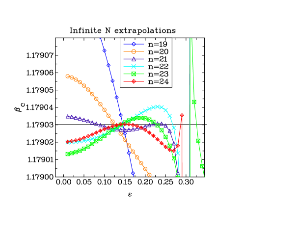
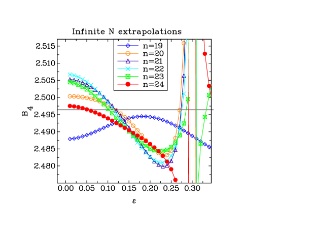
It is important to realize that near the value of where the various curves of figure 4 cross, the extrapolations are approximately the same for all the values of . This means that picking properly allows to get optimally accurate estimates with volumes not too large. One should also appreciate that there are 35 values of in each graph of figure 4 and that for each values of , we need more than 100 calculations of to determine the intersections. Doing the same number of calculations using the MC method for spin models or lattice gauge theory would take a very long time.
5 Comments about the literature
In this section, we comment on existing numerical results found in the literature. We first discuss existing estimates of for the Ising universality class. The methods used can be divided into those that rely on intersections [3, 6], and those that attempt to work as closely as possible to the nontrivial fixed point [5, 7, 8]. Note that [5] takes into account the nonlinear effect of and also the effect of the second irrelevant direction. The results are summarized in table 2. The error bars in [3] are based on the visual estimate from figure 7. The agreement between the two results based on improved action that reduce the effect of the irrelevant variables [7, 8] as well as the agreement with [5] indicates that 1.603 should be accurate with about one part in a 1000. The discrepancy with [6] seems to be of statistical origin: if we use the fit given in equation (14) of [5] together with and we obtain an absolute error less than for if we neglect .
| Model | Ref. | Method | Intersections | |
|---|---|---|---|---|
| Ising 3 | 1.590 (15?) | [3] | MC + reweighting | extrapolation |
| Ising 3 | 1.591 (9) | [6] | MCRG + reweighting | (128,256) |
| Ising 3 | 1.604(1) | [5] | MC at best | - |
| Ising 3 | 1.603(1) | [7] | Improved action | - |
| Ising 3 | 1.603(1) | [8] | Improved action | - |
| 1.620(30) | [11] | MC at various | extrapolation | |
| 1.570(80) | ” | ” | ” | |
| 1.520(100) | ” | ” | ” | |
| 1.622(3) | [16] | MC at various | (24,32) | |
| 1.602(27) | ” | ” | ” | |
| 1.584(39) | ” | ” | ” |
We now discuss the nonlinear effects for specific calculations made with the fixed interval procedure. For the 3 dimensional Ising model, (usually denoted ) is known with great accuracy and consequently, most of the graphs showing use a very narrow interval where the differences between linear fits and numerical data are difficult to see. For instance, if we use the data in figure 6 of [2], it is possible to draw a line that stays within the error bars of all the data points. Consequently, we can only set a lower bound on from this figure by assuming that , defined in B, is less than the error bars that we estimated to be less than 0.02. This bound is consistent with the numerical estimate of [5].
A similar situation is encountered with figure 2 of [16] for LGT with . We focus our analysis on the data points. If we draw a line from the point with the lowest horizontal coordinate to the point with the largest one, the three points inside appear to be above the line. However, the line is within the three error bars. Using the data points kindly provided by the author, we obtained which is slightly less than the errors bars. The lower bound quoted in the table is based on . On the other hand, a clearly non-zero value for can be seen in figure 11 of [4] and figure 9 of [10] and relatively stable values can be obtained for . If we now denote the maximum value of used in the linear fits made to determine the intersections (assuming that such a fits were performed, otherwise we rely on the width of the figure) in each reference, we can estimate the relative size of the nonlinear effects by calculating
| (5.1) |
The numerical values are shown in table 3. There are no large values of . This is because when , the failure of linear fits is obvious. On the other hand, systematic errors due to unaccounted nonlinear effects may be reduced by using a smaller with the procedure discussed in section 3.
6 Conclusions
We have proposed a new method designed to reduce possible nonlinear effects in the estimates of and . For the Ising hierarchical model with a volume corresponding to a linear size of 256 in 3 dimensions, the method gives results which agree with independent accurate estimates with a relative accuracy better than one part in 100,000 for and 5 parts in 1000 for . The intrinsic nonlinear effects (measured in terms of ) in this model are roughly of the same size as those found the other models that we discussed in section 5. Figures 2 and 3 shows the potentially disastrous effect of ignoring nonlinear effects. In graphs with large numerical errors, this effect may be overlooked. The small values of found in the literature indicate that nothing drastic should appear in the cases considered. However, it would be interesting to repeat and extend these calculations for larger volumes using the method proposed here. The optimal value of can in principle be obtained by looking at crossings of extrapolated values. This suggests that the procedure should be followed for a few different values of . We are planning to consider the effects of statistical errors on the new method by applying it to the 3 dimensional Ising model and finite temperature gluodynamics.
Appendix A Numerical Calculations
For completeness, we explain how we calculated for the hierarchical model and we give the details of the numerical calculations of the parameters. The interest of the hierarchical model is that we can blockspin exactly. The basic formula for the Fourier transform of the local measure is
| (1.1) |
with
| (1.2) |
Note that we do not rescale the field as in a renormalization group transformation. is a constant that we adjust so that . When it is the case, we have
| (1.3) |
with the sum of all the spins. If we write
| (1.4) |
Then
| (1.5) |
The critical values are obtained by plugging the values of and from the nontrivial fixed point. See [22] for details and references. The value of is obtained by increasing but keeping constant. The asymptotic values for different can be fitted very well with a line which gives and . We then subtracted the effect of and obtained and using discrete derivatives near .
We used calculations at very large volume (). In the text, we show that these accurate results can be reproduced with a new procedure using data at much smaller volume. From Refs. [20, 21],
| (1.6) | |||||
Using these values, and numerical results a fixed values of and large , we first determine the terms and find
| (1.7) |
Subtracting these effect and taking discrete approximation of the derivative with respect to near 0, we find
| (1.8) |
One should appreciate that we have been able to determine numerically the 8 parameters of equation (2.7) with good numerical stability.
Appendix B Estimate of the nonlinear effects with pencil and ruler
In this appendix, we explain how to estimate the order of magnitude of from a graph illustrating approximate data collapse such as figure 1, using a pencil and a ruler. A subset of the data of figure 1 is shown in figure 5 together with lines that can be drawn on the original graph. The line joins two points with approximately opposite coordinates. We denote these two points and . We call the difference between the line and the data (assumed to be a quadratic function) at 0 . It is then easy to show that
| (2.1) |
In figure 5, we have approximately , , and , which gives the estimates and which are in reasonably good agreement with the previous estimates. Note that we are mostly interested in the ratio and that this ratio is invariant under a multiplicative rescaling. This is useful if we are considering graphs with other quantities displayed (for instance ). For the model considered here, .
The above estimates are based on the data with . In figure 5, we also see part of the data for and we see that it is not much above the data. From equation (2.7), it is clear that if we neglect , the entire curve is translated uniformly in the vertical direction. But the estimates of and are based on differences and do not depend on this translation provided that we only use data for one value of . This is confirmed by using the data as shown in figure 5 where we obtain an estimate of very close to the one quoted above for . This shows that up to a subtraction and rescaling of the horizontal coordinate, we can rely on a graph of versus at relatively small volume. It is clear that the subtraction of requires to have an estimate of this quantity. However, this estimate does not need to be very precise to get the order of magnitude of .


References
References
- [1] Binder K 1981 Z. Phys. B43 119–140
- [2] Barber M N, Pearson R B, Toussaint D and Richardson J L 1985 Phys. Rev. B 32 1720–1730
- [3] Ferrenberg A M and Landau D P 1991 Phys. Rev. B 44 5081–5091
- [4] Olsson P 1997 Phys. Rev. B 55 3585–3602
- [5] Blote H, Luitgen E and Heringa J 1996 J. Phys. A 28 6289–6313
- [6] Gupta R and Tamayo P 1996 Int. Jour. of Mod. Phys. C 7 305–319
- [7] Hasenbusch M, Pinn K and Vinti S 1998 Physical Review B 59 11471
- [8] Campostrini M, Pelissetto A, Rossi P and Vicari E 1999 Phys. Rev. E60 3526–3563
- [9] Binder K and Luijten E 2001 Phys. Rept. 344 179–253
- [10] Engels J, Fingberg J and Weber M 1990 Nucl. Phys. B332 737
- [11] Fingberg J, Heller U M and Karsch F 1993 Nucl. Phys. B392 493–517
- [12] Sinclair D K and Kogut J B 2006 PoS LAT2006 147 (Preprint hep-lat/0609041)
- [13] Sinclair D K and Kogut J B 2007 (Preprint arXiv:0709.2367 [hep-lat])
- [14] de Forcrand P, Stephanov M A and Wenger U 2007 (Preprint arXiv:0711.0023 [hep-lat])
- [15] de Forcrand P, Kim S and Philipsen O 2007 (Preprint arXiv:0711.0262 [hep-lat])
- [16] Velytsky A 2007 (Preprint arXiv:0711.0748 [hep-lat])
- [17] Meurice Y and Oktay B in progress
- [18] Dyson F 1969 Comm. Math. Phys. 12 91
- [19] Godina J, Meurice Y, Oktay M and Niermann S 1998 Phys. Rev. D 57 6326
- [20] Godina J, Meurice Y and Oktay M 1998 Phys. Rev. D 57 R6581
- [21] Godina J, Meurice Y and Oktay M 1999 Phys. Rev. D 59 096002
- [22] Meurice Y 2007 J. Phys. A40 R39
- [23] Campbell I A, Hukushima K and Takayama H 2006 Physical Review Letters 97 117202
- [24] Campbell I A, Hukushima K and Takayama H 2007 Physical Review B 76 134421