Detecting changes in the fluctuations of a Gaussian process and an application to heartbeat time series

Abstract

The aim of this paper is first the detection of multiple abrupt changes of the long-range dependence (respectively self-similarity, local fractality) parameters from a sample of a Gaussian stationary times series (respectively time series, continuous-time process having stationary increments). The estimator of the $m$ change instants (the number $m$ is supposed to be known) is proved to satisfied a limit theorem with an explicit convergence rate. Moreover, a central limit theorem is established for an estimator of each long-range dependence (respectively self-similarity, local fractality) parameter. Finally, a goodness-of-fit test is also built in each time domain without change and proved to asymptotically follow a Khi-square distribution. Such statistics are applied to heart rate data of marathon’s runners and lead to interesting conclusions.

Keywords: Long-range dependent processes; Self-similar processes; Detection of abrupt changes; Hurst parameter; Self-similarity parameter; Wavelet analysis; Goodness-of-fit test.

1 Introduction

The content of this paper was motivated by a general study of physiological signals of runners recorded during endurance races as marathons. More precisely, after different signal procedures for "cleaning" data, one considers the time series resulting of the evolution of heart rate (HR data in the sequel) during the race. The following figure provides several examples of such data (recorded during Marathon of Paris 2004 by Professor V. Billat and her laboratory LEPHE, see http://www.billat.net). For each runner, the periods (in ms) between the successive pulsations (see Fig. 1) are recorded. The HR signal in number of beats per minute (bpm) is then deduced (the HR average for the whole sample is of 162 bpm).

Figure 1: Heat rate signals of Athlete 1 in ms, Hertz and BPM (up), of Athletes 2, 3 and 4 in BPM (down)

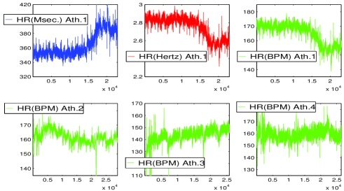
Numerous authors have studied heartbeat time series (see for instance [24], [25] or [3]). A model proposed to fit these data is a trended long memory process with an estimated Hurst parameter close to $1$ (and sometimes more than $1$). In [17] three improvements have been proposed to such a model: 1/ data are stepped in three different stages which are detected using a change point’s detection method (see for instance [19] or [21]). The main idea of the detection’s method is to consider that the signal distribution depends on a vector of unknown characteristic parameters constituted by the mean and the variance. The different stages (beginning, middle and end of the race) and therefore the different vectors of parameters, which change at two unknown instants, are estimated. 2/ during each stage, a time-continuous Gaussian process is proposed for modelling the detrended time series. This process is a generalization of a fractional Gaussian noise (FGN) also called locally fractional Gaussian noise such that, roughly speaking, there exists a local-fractality parameter $H\in\mathds{R}$ (corresponding to Hurst parameter for FGN) only for frequencies $|\xi|\in[f_{min}\,,\,f_{max}]$ with $0<f_{min}<f_{max}$ (see more details below). 3/ this parameter $H$ which is very interesting for interpreting and explaining the physiological signal behaviours, is estimating from a wavelet analysis. Rigorous results are also proved providing a central limit theorem satisfied by the estimator.
In order to improve this study of HR data and since the eventual changes of $H$ values are extremely meaningful for explaining the eventual physiological changes of the athlete’s HR during the race, the detection of abrupt change of $H$ values is the aim of this paper. By this way the different stages detected during the race will be more relevant for explaining the physiological status of the athlete than stages detected from changes in mean or variance. For instance, the HR of a runner could decrease in mean even if the "fluctuations" of the HR does not change.
 
In this paper, an estimator of $m$ instants ($m\in\mathds{N}^{*}$) of abrupt changes of long-range dependence, self-similarity or local-fractality (more details about these terms will be provided below) is developed for a sample of a Gaussian process. Roughly speaking, the principle of such estimator is the following: in each time’s domain without change, the parameter of long-range dependence (or self-similarity or local self-fractality) can be estimated from a log-log regression of wavelet coefficients’ variance onto several chosen scales. Then a contrast defined by the sum on every $m+1$ possible zones of square distances between points and regressions lines is minimized providing an estimator of the $m$ instants of change. Under general assumptions, a limit theorem with a convergence rate satisfied by such an estimator is established in Theorem 2.1.
Moreover, in each estimated no-change zone, parameters of long-range dependence (or self-similarity or local self-similarity) can be estimated, first with an ordinary least square (OLS) regression, secondly with a feasible generalized least square (FGLS) regression. Central limit theorems are established for both these estimators (see Theorem 2.2 and Proposition 2.3 below) and confidence intervals can therefore be computed. The FGLS estimator provides two advantages: from the one hand, its asymptotic variance is smaller than OLS estimator one. From the other hand, it allows to construct a very simple (Khi-square) goodness-of-fit test based on a squared distance between points and FGLS regression line. The asymptotic behavior of this test is provided in Theorem 2.4.
 
Then, different particular cases of Gaussian processes are studied:

1. long-range dependent processes with abrupt changes of values of LRD parameters. In such time series case, a semi-parametric frame is supposed (including fractional Gaussian noises (FGN) and Gaussian FARIMA processes) and assumptions of limit theorems are always satisfied with interesting convergence rates (see Corollary 3.2).

2. self-similar time series with abrupt changes of values of self-similarity parameters. In such case, fractional Brownian motions (FBM) are only considered. Surprisingly, convergences of estimators are only established when the maximum of differences between self-similarity parameters is sufficiently small. Simulations exhibit a non convergence of the estimator of instant change when a difference between two parameters is too large (see Corollary 3.4).

3. locally fractional Gaussian processes with abrupt changes of values of local-fractality parameters. In such a continuous time processes’ case, a semi-parametric frame is supposed (including multiscale fractional Brownian motions) and assumptions of limit theorems are always satisfied with interesting convergence rates (see Corollary 3.6).

The problem of change-point detection using a contrast minimization was first studied in the case of independent processes (see for instance Bai and Perron [5]), then for weakly dependent processes (see for instance Bai [4], Lavielle [19] or Lavielle and Moulines [20]) and since middle of 90’s in the case of processes which exhibit long-range dependance (see for instance Giraitis et al. [13], Kokoszka and Leipus [18] or Lavielle and Teyssière [21]). Of the various approaches, some were associated with a parametric framework for a change points detection in mean and/or variance and others where associated with a non-parametric framework (typically like detecting changes in distribution or spectrum). To our knowledge, the semi-parametric case of abrupt change detection for long-range dependent or self-similarity parameter is treated here for the first time.
However, in the literature different authors have proposed test statistics for testing the no-change null hypothesis against the alternative that the long-memory parameter changes somewhere in the observed time series. Beran and Terrin [10] proposed an approach based on the Whittle estimator, Horváth and Shao [16] obtained limit distribution of the test statistic based on quadratic forms and Horváth [15] suggested another test based on quadratic forms of Whittle estimator of long-memory parameter. The goodness-of-fit test presented below and which satisfies the limit theorem 2.4 also allows to test if the long-range memory (or self-similarity or local-fractality) parameter changes somewhere in the time series.
 
Our approach is based on the wavelet analysis. This method applied to LRD or self-similar processes for respectively estimating the Hurst or self-similarity parameter was introduced by Flandrin [12] and was developed by Abry, Veitch and Flandrin [2] and Bardet et al. [9]. The convergence of wavelet analysis estimator was studied in the case of a sample of FBM in [6], and in a semi-parametric frame of a general class of stationary Gaussian LRD processes by Moulines et al. [22] and Bardet et al. [9]. Moreover, wavelet based estimators are robust in case of polynomial trended processes (see Corollary 2.1) and is therefore very interesting for studying stochastic fluctuations of a process without taking care on its smooth variations.
A method based on wavelet analysis was also developed by Bardet and Bertrand [7] in the case of multiscale FBM (a generalization of the FBM for which the Hurst parameter depends on the frequency as a piecewise constant function) providing statistics for the identification (estimation and goodness-of-fit test) of such a process. Such a process was used for modelling biomechanics signals. In the same way, the locally fractional Gaussian process (a generalization of the FBM for which the Hurst parameter, called the local-fractality parameter, is constant in a given domain of frequencies) was studied in [17] for modelling HR data during the three characteristics stages of the race. An increasing evolution of the local-fractality parameter during the race was generally showed for any runner from this method. Using the method of abrupt change detection of local-fractality parameter $H$ developed in Corollary 3.6, this result is confirmed by estimations of $H$ for each runner even if the change’s instants seem to vary a lot depending on the fatigue of the runner (see the application to HR’s time series in Section 3).
 
The paper is organized as follows. In Section 2, notations, assumptions and limit theorems are provided in a general frame. In Section 3, applications of the limit theorems to three kind of "piecewise" Gaussian process are presented with also simulations. The case of HR data is also treated. Section 4 is devoted to the proofs.

2 Main results

2.1 Notations and assumptions

First, a general and formal frame can be proposed. Let $(X_{t})_{t\in T}$ be a zero-mean Gaussian process with $T=\mathds{N}$ or $T=\mathds{R}$ and assume that

$$\big{(}X_{0},X_{\delta_{N}},X_{2\delta_{N}},\ldots,X_{N\delta_{N}}\big{)}~{}~{}\mbox{is known with $\delta_{N}=1$ or $\delta_{N}\begin{array}[t]{c}\stackrel{{\scriptstyle}}{{\longrightarrow}}\\ {\scriptstyle N\rightarrow\infty}\end{array}0$,}$$

following data are modeled with a time series ($T=\mathds{N}$) or a continuous time process $T=\mathds{R}$. In the different proposed examples $X$ could be a stationary long memory time series or a self-similar or locally fractional process having stationary increments.
For estimations using a wavelet based analysis, consider $\psi:\mathds{R}\rightarrow\mathds{R}$ a function called "the mother wavelet". In applications, $\psi$ is a function with a compact (for instance Daubeshies wavelets) or an essentially compact support (for instance Lemarié-Meyer wavelets). For $(X_{t})_{t\in T}$ and $(a,b)\in\mathds{R}_{+}^{*}\times\mathds{R}$, the wavelet coefficient of $X$ for the scale $a$ and the shift $b$ is

$$d_{X}(a,b):=\frac{1}{\sqrt{a}}\int_{\mathds{R}}\psi(\frac{t-b}{a})X(t)dt.$$

When only a discretized path of $X$ is available (or when $T=\mathds{N}$), approximations $e_{X}(a,b)$ of $d_{X}(a,b)$ are only computable. We have chosen to consider for $(a,b)\in\mathds{R}_{+}^{*}\times\mathds{N}$,

$$e_{X}(a,b):=\frac{\delta_{n}}{\sqrt{a}}\,\sum_{p=1}^{N}\psi\big{(}\frac{p-b}{a}\big{)}X_{p\,\delta_{N}},$$ (1)

which is the formula of wavelet coefficients computed from Mallat’s algorithm for compactly supported discrete ($a\in 2^{\mathds{N}}$) wavelet transform (for instance Daubeshies wavelets) when $N$ is large enough and nearly this formula for discrete wavelet transform with an essentially compact support (for instance Lemarié-Meyer wavelets). Now assume that there exist $m\in\mathds{N}$ (the number of abrupt changes) and

• $0=\tau_{0}^{*}<\tau_{1}^{*}<\ldots<\tau_{m}^{*}<\tau_{m+1}^{*}=1$ (unknown parameters);

• two families $(\alpha_{j}^{*})_{0\leq j\leq m}\in\mathds{R}^{m+1}$ and $(\beta_{j}^{*})_{0\leq j\leq m}\in(0,\infty)^{m+1}$ (unknown parameters);

• a sequence of "scales" $(a_{n})_{n\in\mathds{N}}\in\mathds{R}^{\mathds{N}}$ (known sequence) satisfying $a_{n}\geq a_{min}$ for all $n\in\mathds{N}$, with $a_{min}>0$,

such that for all $j=0,1,\ldots,m$ and $k\in D_{N}^{*}(j)\subset\big{[}[N\delta_{N}\tau_{j}^{*}]\,,\,[N\delta_{N}\tau_{j+1}^{*}]\big{]}$,

$$\mathds{E}\big{[}e_{X}^{2}(a_{N},k)\big{]}\sim\beta_{j}^{*}\cdot\big{(}a_{N}\big{)}^{\alpha_{j}^{*}}~{}~{}\mbox{when}~{}~{}N\to\infty\mbox{ and }N\delta_{N}\to\infty.$$ (2)

Roughly speaking, for $N\in\mathds{N}^{*}$ the change instants are $[N\delta_{N}\tau_{j}^{*}]$ for $j=1,\ldots,m$, the variance of wavelet coefficients follows a power law of the scale, and this power law is piecewise varying following the shift. Thus piecewise sample variances can be appropriated estimators of parameters of these power laws. Hence let us define

$$S^{k^{\prime}}_{k}(a_{N}):=\frac{a_{N}}{k^{\prime}-k}\,\sum_{p=[k/a_{N}]}^{[k^{\prime}/a_{N}]-1}e_{X}^{2}(a_{N},a_{N}\,p)~{}~{}\mbox{for $0\leq k<k^{\prime}\leq N\delta_{N}$}.$$ (3)

Now set $0<r_{1}<\ldots<r_{\ell}$ with $\ell\in\mathds{N}^{*}$ and let us suppose that a multidimensional central limit theorem can also be established for $\big{(}S^{k^{\prime}}_{k}(r_{i}\,a_{N})\big{)}_{1\leq i\leq\ell}$, i.e.

$$\big{(}S^{k^{\prime}}_{k}(r_{i}\,a_{N})\big{)}_{1\leq i\leq\ell}=\big{(}\beta_{j}^{*}\cdot\big{(}r_{i}\,a_{N}\big{)}^{\alpha_{j}^{*}}\big{)}_{1\leq i\leq\ell}+\big{(}a_{N}\big{)}^{\alpha_{j}^{*}}\times\sqrt{\frac{a_{N}}{k^{\prime}-k}}\,\big{(}\varepsilon_{i}^{(N)}(k,k^{\prime})\big{)}_{1\leq i\leq\ell},$$ (4)

with $[N\delta_{N}\tau_{j}^{*}]\leq k<k^{\prime}\leq[N\delta_{N}\tau_{j+1}^{*}]$ and it exists $\Gamma^{(j)}(\alpha_{j}^{*},r_{1},\ldots,r_{\ell})=\big{(}\gamma_{pq}^{(j)}\big{)}_{1\leq p,q\leq\ell}$ a $(\ell\times\ell)$ matrix not depending on $N$ such that $\alpha\mapsto\Gamma^{(j)}(\alpha,r_{1},\ldots,r_{\ell})$ is a continuous function, a positive matrix for all $\alpha$ and

$$\big{(}\varepsilon_{i}^{(N)}(k,k^{\prime})\big{)}_{1\leq i\leq\ell}\begin{array}[t]{c}\stackrel{{\scriptstyle{\mathcal{L}}}}{{\longrightarrow}}\\ {\scriptstyle N\rightarrow\infty}\end{array}\mathcal{N}\big{(}0,\Gamma^{(j)}(\alpha_{j}^{*},r_{1},\ldots,r_{\ell})\big{)}~{}~{}\mbox{when}~{}~{}k^{\prime}-k\to\infty.$$ (7)

With the usual Delta-Method, relation (4) implies that for $1\leq i\leq\ell$,

$$\log\big{(}S^{k^{\prime}}_{k}(r_{i}\,a_{N})\big{)}=\log(\beta_{j}^{*})+\alpha_{j}^{*}\log\big{(}r_{i}\,a_{N}\big{)}+\sqrt{\frac{a_{N}}{k^{\prime}-k}}\,\varepsilon_{i}^{(N)}(k,k^{\prime}),$$ (8)

for $[N\delta_{N}\tau_{j}^{*}]\leq k<k^{\prime}\leq[N\delta_{N}\tau_{j+1}^{*}]$ and the limit theorem (7) also holds. This is a linear model and therefore a log-log regression of $\big{(}S^{k^{\prime}}_{k}(r_{i}\,a_{N})\big{)}_{i}$ onto $\big{(}r_{i}\,a_{N}\big{)}_{i}$ provides an estimator of $\alpha_{j}^{*}$ and $\log(\beta_{j}^{*})$.
 
The first aim of this paper is the estimation of unknown parameters $(\tau_{j}^{*})_{j}$, $(\alpha_{j}^{*})_{j}$ and $(\beta_{j}^{*})_{j}$. Therefore, define a contrast function

$$U_{N}\big{(}(\alpha_{j})_{0\leq j\leq m},\,(\beta_{j})_{0\leq j\leq m},\,(k_{j})_{1\leq j\leq m}\big{)}=\sum_{j=0}^{m}\sum_{i=1}^{\ell}\Big{(}\log\big{(}S^{k_{j+1}}_{k_{j}}(r_{i}\,a_{N})\big{)}-\big{(}\alpha_{j}\log(r_{i}\,a_{N})+\log\beta_{j}\big{)}\Big{)}^{2}\\ \mbox{with}~{}~{}~{}~{}\left\{\begin{array}[]{l}\bullet~{}(\alpha_{j})_{0\leq j\leq m}\in A^{m+1}\subset\mathds{R}^{m+1}\\ \bullet~{}(\beta_{j})_{0\leq j\leq m}\in B^{m+1}\subset(0,\infty)^{m+1}\\ \bullet~{}0=k_{0}<k_{1}<\ldots<k_{m}<k_{m+1}=N\delta_{N},(k_{j})_{1\leq j\leq m}\in K_{m}(N)\subset\mathds{R}^{m}\end{array}\right..$$

The vector of estimated parameters $\widehat{\alpha}_{j},~{}\widehat{\beta}_{j}$ and $\widehat{k}_{j}$ (and therefore $\widehat{\tau}_{j}$) is the vector which minimizes this contrast function, i.e.,

$$\big{(}(\widehat{\alpha}_{j})_{0\leq j\leq m},\,(\widehat{\beta}_{j})_{0\leq j\leq m},\,(\widehat{k}_{j})_{1\leq j\leq m}\big{)}$$ (9)

$$:=\text{Argmin}\Big{\{}U_{N}\big{(}(\alpha_{j})_{0\leq j\leq m},\,(\beta_{j})_{0\leq j\leq m},\,(k_{j})_{1\leq j\leq m}\big{)}\Big{\}}~{}~{}\mbox{in}~{}~{}A^{m+1}\times B^{m+1}\times K_{m}(N)$$

$$\widehat{\tau}_{j}\hskip 156.49014pt :=\widehat{k}_{j}/(N\delta_{N})~{}~{}\mbox{for}~{}~{}1\leq j\leq m.$$ (10)

For a given $(k_{j})_{1\leq j\leq m}$, it is obvious that $(\widehat{\alpha}_{j})_{0\leq j\leq m}$ and $(\log\widehat{\beta}_{j})_{0\leq j\leq m}$ are obtained from a log-log regression of $\big{(}S^{k_{j+1}}_{k_{j}}(r_{i}\,a_{N})\big{)}_{i}$ onto $\big{(}r_{i}\,a_{N}\big{)}_{i}$, i.e.

$$\left(\begin{array}[]{c}\widehat{\alpha}_{j}\\ \log\widehat{\beta}_{j}\end{array}\right)=\big{(}L_{1}^{\prime}\cdot L_{1})^{-1}L_{1}^{\prime}\cdot Y_{k_{j}}^{k_{j+1}}$$

with $\displaystyle{Y_{k_{j}}^{k_{j+1}}:=\big{(}\log\big{(}S^{k_{j+1}}_{k_{j}}(r_{i}\cdot a_{N})\big{)}\big{)}_{1\leq i\leq\ell}}$ and $\displaystyle{L_{a_{N}}:=\left(\begin{array}[]{cc}\log(r_{1}\,a_{N})&1\\ \vdots&\vdots\\ \log(r_{\ell}\,a_{N})&1\end{array}\right).}$ Therefore the estimator of the vector $(k_{j})_{1\leq j\leq m}$ is obtained from the minimization of the contrast

$$G_{N}(k_{1},k_{2},\ldots,k_{m}) := U_{N}\big{(}(\widehat{\alpha}_{j})_{0\leq j\leq m},\,(\widehat{\beta}_{j})_{0\leq j\leq m},\,(k_{j})_{1\leq j\leq m}\big{)}$$ (12)

$$\Longrightarrow~{}~{}(\widehat{k}_{j})_{1\leq j\leq m}=\text{Argmin}\Big{\{}G_{N}(k_{1},k_{2},\ldots,k_{m}),~{}~{}(k_{j})_{1\leq j\leq m}\in K_{m}(N)\Big{\}}.$$

2.2 Estimation of abrupt change time-instants $(\tau_{j}^{*})_{1\leq j\leq m}$

In this paper, parameters $(\alpha_{j}^{*})$ are supposed to satisfied abrupt changes. Such an hypothesis is provided by the following assumption:
 
Assumption C: Parameters $(\alpha_{j}^{*})$ are such that $|\alpha_{j+1}^{*}-\alpha_{j}^{*}|\neq 0~{}~{}\mbox{for all}~{}~{}j=0,1,\ldots,m-1.$
 
Now let us define:

$$\underline{\tau}^{*}:=(\tau^{*}_{1},\ldots,\tau^{*}_{m}),~{}~{}\underline{\widehat{\tau}}:=(\widehat{\tau}_{1},\ldots,\widehat{\tau}_{m})~{}~{}\mbox{and}~{}~{}\|\underline{\tau}\|_{m}:=\max\big{(}|\tau_{1}|,\ldots,|\tau_{m}|\big{)}.$$

Then $\underline{\widehat{\tau}}$ converges in probability to $\underline{\tau}^{*}$ and more precisely,

Theorem 2.1

Let $\ell\in\mathds{N}\setminus\{0,1,2\}$. If Assumption C and relations (4), (7) and (8) hold with $(\alpha_{j}^{*})_{0\leq j\leq m}$ such that $\alpha_{j}^{*}\in[a\,,\,a^{\prime}]$ and $a<a^{\prime}$ for all $j=0,\ldots,m$, then if $\displaystyle~{}~{}a_{N}^{1+2(a^{\prime}-a)}(N\,\delta_{N})^{-1}\begin{array}[t]{c}\stackrel{{\scriptstyle}}{{\longrightarrow}}\\ {\scriptstyle N\rightarrow\infty}\end{array}0$, for all $(v_{n})_{n}$ satisfying $\displaystyle~{}~{}v_{N}\cdot a_{N}^{1+2(a^{\prime}-a)}(N\,\delta_{N})^{-1}\begin{array}[t]{c}\stackrel{{\scriptstyle}}{{\longrightarrow}}\\ {\scriptstyle N\rightarrow\infty}\end{array}0$,

$$\mathds{P}\Big{(}v_{N}\|\underline{\tau}^{*}-\underline{\widehat{\tau}}\|_{m}\geq\eta\Big{)}\begin{array}[t]{c}\stackrel{{\scriptstyle}}{{\longrightarrow}}\\ {\scriptstyle N\rightarrow\infty}\end{array}0~{}~{}~{}\mbox{for all $\eta>0$}.$$ (15)

Several examples of applications of this theorem will be seen in Section 3.

2.3 Estimation of parameters $(\alpha_{j}^{*})_{0\leq j\leq m}$ and $(\beta_{j}^{*})_{0\leq j\leq m}$

For $j=0,1,\ldots,m$, the log-log regression of $\big{(}S_{\widehat{k}_{j}}^{\widehat{k}_{j+1}}(r_{i}a_{N})\big{)}_{1\leq i\leq\ell}$ onto $(r_{i}a_{N})_{1\leq i\leq\ell}$ provides the estimators of $\alpha_{j}^{*}$ and $\beta_{j}^{*}$. However, even if $\tau_{j}$ converges to $\tau_{j}^{*}$, $\widehat{k}_{j}=N\delta_{N}\cdot\widehat{\tau}_{j}$ does not converge to $k_{j}^{*}$ (except if $N=o(v_{N})$ which is quite impossible), and therefore $\mathds{P}\big{(}[\widehat{k}_{j},\widehat{k}_{j+1}]\subset[k^{*}_{j},k^{*}_{j+1}]\big{)}$ does not tend to $1$. So, for $j=0,1,\ldots,m$, define $\tilde{k}_{j}$ and $\tilde{k}_{j}^{\prime}$ such that

$$\tilde{k}_{j}=\widehat{k}_{j}+\frac{N\delta_{N}}{v_{N}}~{}~{}~{}\mbox{and}~{}~{}~{}\tilde{k}_{j}^{\prime}=\widehat{k}_{j+1}-\frac{N\delta_{N}}{v_{N}}~{}~{}\Longrightarrow~{}~{}\mathds{P}\big{(}[\tilde{k}_{j},\tilde{k}_{j}^{\prime}]\subset[k^{*}_{j},k^{*}_{j+1}]\big{)}\begin{array}[t]{c}\stackrel{{\scriptstyle}}{{\longrightarrow}}\\ {\scriptstyle N\rightarrow\infty}\end{array}1,$$

from (15) with $\eta=1/2$. Let $\Theta^{*}_{j}:=\left(\begin{array}[]{c}\alpha^{*}_{j}\\ \log\beta^{*}_{j}\\ \end{array}\right)$ and $\tilde{\Theta}_{j}:=(L_{1}^{{}^{\prime}}\cdot L_{1})^{-1}L_{1}^{{}^{\prime}}\cdot Y_{\tilde{k}_{j}}^{\tilde{k}_{j}^{\prime}}:=\left(\begin{array}[]{c}\tilde{\alpha}_{j}\\ \log\tilde{\beta}_{j}\\ \end{array}\right)$. Thus, estimators $(\tilde{\alpha}_{j})_{0\leq j\leq m}$ and $(\tilde{\beta}_{j})_{0\leq j\leq m}$ satisfy

Theorem 2.2

Under the same assumptions as in Theorem 2.1, for $j=0,\ldots,m$

$$\sqrt{\frac{\delta_{N}\,N\big{(}\tau^{*}_{j+1}-\tau^{*}_{j}\big{)}}{a_{N}}}\Big{(}\tilde{\Theta}_{j}-\Theta^{*}_{j}\Big{)}\begin{array}[t]{c}\stackrel{{\scriptstyle{\mathcal{L}}}}{{\longrightarrow}}\\ {\scriptstyle N\rightarrow\infty}\end{array}\mathcal{N}\big{(}0,\Sigma^{(j)}(\alpha_{j}^{*},r_{1},\ldots,r_{\ell})\big{)}$$ (18)

with $\Sigma^{(j)}(\alpha_{j}^{*},r_{1},\ldots,r_{\ell}):=(L_{1}^{{}^{\prime}}\cdot L_{1})^{-1}L_{1}^{{}^{\prime}}\cdot\Gamma^{(j)}(\alpha_{j}^{*},r_{1},\ldots,r_{\ell})\cdot L_{1}\cdot(L_{1}^{{}^{\prime}}\cdot L_{1})^{-1}$.

A second estimator of $\Theta^{*}_{j}$ can be obtained from feasible generalized least squares (FGLS). Indeed, the asymptotic covariance matrix $\Gamma^{(j)}(\alpha_{j}^{*},r_{1},\ldots,r_{\ell})$ can be estimated with the matrix $\tilde{\Gamma}^{(j)}:=\Gamma^{(j)}(\tilde{\alpha}_{j},r_{1},\ldots,r_{\ell})$ and $\tilde{\Gamma}^{(j)}\begin{array}[t]{c}\stackrel{{\scriptstyle{\mathcal{P}}}}{{\longrightarrow}}\\ {\scriptstyle N\rightarrow\infty}\end{array}\Gamma^{(j)}(\alpha_{j}^{*},r_{1},\ldots,r_{\ell})$ since $\alpha\mapsto\Gamma^{(j)}(\alpha,r_{1},\ldots,r_{\ell})$ is supposed to be a continuous function and $\tilde{\alpha}_{j}\begin{array}[t]{c}\stackrel{{\scriptstyle{\mathcal{P}}}}{{\longrightarrow}}\\ {\scriptstyle N\rightarrow\infty}\end{array}\alpha^{*}_{j}$. Since also $\alpha\mapsto\Gamma^{(j)}(\alpha,r_{1},\ldots,r_{\ell})$ is supposed to be a positive matrix for all $\alpha$ then

$$\Big{(}\tilde{\Gamma}^{(j)}\Big{)}^{-1}\begin{array}[t]{c}\stackrel{{\scriptstyle{\mathcal{P}}}}{{\longrightarrow}}\\ {\scriptstyle N\rightarrow\infty}\end{array}\Big{(}\Gamma^{(j)}(\alpha_{j}^{*},r_{1},\ldots,r_{\ell})\Big{)}^{-1}.$$

Then, the FGLS estimator ${\overline{\Theta}}_{j}$ of $\Theta^{*}_{j}$ is defined from the minimization for all $\Theta$ of the following criterion

$$\parallel Y_{\tilde{k}_{j}}^{\tilde{k}_{j}^{\prime}}-L_{a_{N}}\cdot\Theta\parallel^{2}_{\tilde{\Gamma}^{(j)}}=\big{(}Y_{\tilde{k}_{j}}^{\tilde{k}^{\prime}_{j}}-L_{a_{N}}\cdot\Theta\big{)}^{\prime}\cdot\big{(}\tilde{\Gamma}^{(j)}\big{)}^{-1}\cdot\big{(}Y_{\tilde{k}_{j}}^{\tilde{k}_{j}^{\prime}}-L_{a_{N}}\cdot\Theta\big{)}.$$

and therefore

$${\overline{\Theta}}_{j}=\big{(}L_{1}^{\prime}\cdot\big{(}\tilde{\Gamma}^{(j)}\big{)}^{-1}\cdot L_{1}\big{)}^{-1}\cdot L_{1}^{\prime}\cdot\big{(}\tilde{\Gamma}^{(j)}\big{)}^{-1}\cdot Y_{\tilde{k}_{j}}^{\tilde{k}_{j}^{\prime}}.$$

Proposition 2.3

Under the same assumptions as in Theorem 2.2, for $j=0,\ldots,m$

$$\sqrt{\frac{\delta_{N}\,N\big{(}\tau^{*}_{j+1}-\tau^{*}_{j}\big{)}}{a_{N}}}\Big{(}{\overline{\Theta}}_{j}-\Theta^{*}_{j}\Big{)}\begin{array}[t]{c}\stackrel{{\scriptstyle{\mathcal{L}}}}{{\longrightarrow}}\\ {\scriptstyle N\rightarrow\infty}\end{array}\mathcal{N}\big{(}0,M^{(j)}(\alpha_{j}^{*},r_{1},\ldots,r_{\ell})\big{)}$$ (21)

with $M^{(j)}(\alpha_{j}^{*},r_{1},\ldots,r_{\ell}):=\big{(}L_{1}^{{}^{\prime}}\cdot\big{(}\Gamma^{(j)}(\alpha_{j}^{*},r_{1},\ldots,r_{\ell})\big{)}^{-1}\cdot L_{1}\big{)}^{-1}\leq\Sigma^{(j)}(\alpha_{j}^{*},r_{1},\ldots,r_{\ell})$ (with order’s relation between positive symmetric matrix).

Therefore, the estimator ${\overline{\Theta}}_{j}$ converges asymptotically faster than $\tilde{\Theta}_{j}$; ${\overline{\alpha}}_{j}$ is more interesting than $\tilde{\alpha}_{j}$ for estimating $\alpha_{j}^{*}$ when $N$ is large enough. Moreover, confidence intervals can be easily deduced for both the estimators of $\Theta^{*}_{j}$.

2.4 Goodness-of-fit test

For $j=0,\ldots,m$, let $T^{(j)}$ be the FGLS distance between both the estimators of $L_{a_{N}}\cdot\Theta^{*}_{j}$, i.e. the FGLS distance between points $\Big{(}\log(r_{i}\,a_{N}),\log\big{(}S^{\tilde{k}_{j}^{\prime}}_{\tilde{k}_{j}}\big{)}\Big{)}_{1\leq i\leq\ell}$ and the FGLS regression line. The following limit theorem can be established:

Theorem 2.4

Under the same assumptions as in Theorem 2.1, for $j=0,\ldots,m$

$$T^{(j)}=\frac{\delta_{N}\,N\big{(}\tau^{*}_{j+1}-\tau^{*}_{j}\big{)}}{a_{N}}\parallel Y_{\tilde{k}_{j}}^{\tilde{k}_{j}^{\prime}}-L_{a_{N}}\cdot{\overline{\Theta}}_{j}\parallel^{2}_{\tilde{\Gamma}^{(j)}}\begin{array}[t]{c}\stackrel{{\scriptstyle{\mathcal{L}}}}{{\longrightarrow}}\\ {\scriptstyle N\rightarrow\infty}\end{array}\chi^{2}(\ell-2).$$ (24)

Mutatis mutandis, proofs of Proposition 2.3 and Theorem 2.4 are the same as the proof of Proposition 5 in [7]. This test can be applied to each segment $[\tilde{k}_{j},\tilde{k}_{j}^{\prime}[$. However, under the assumptions, it is not possible to prove that a test based on the sum of $T^{(j)}$ for $j=0,\ldots,m$ converges to a $\chi^{2}\big{(}(m+1)(\ell-2)\big{)}$ distribution (indeed, nothing is known about the eventual correlation of $\big{(}Y_{\tilde{k}_{j}}^{\tilde{k}_{j}^{\prime}}\big{)}_{0\leq j\leq m}$).

2.5 Cases of polynomial trended processes

Wavelet based estimators are also known to be robust to smooth trends (see for instance [1]). More precisely, assume now that one considers the process $Y=\{Y_{t},t\in T\}$ satisfying $Y_{t}=X_{t}+P(t)$ for all $t\in T$ where $P$ is an unknown polynomial function of degree $p\in\mathds{N}$. Then,

Corollary 2.1

Under the same assumptions as in Theorem 2.1 for the process $X$, and if the mother wavelet $\psi$ is such that $\int t^{r}\,\psi(t)dt=0$ for $r=0,1,\ldots,p$, then limit theorems (4), (7) and (8) hold for $X$ and for $Y$.

Let us remark that Lemarié-Meyer wavelet is such that $\int t^{r}\,\psi(t)dt=0$ for all $r\in\mathds{N}$. Therefore, even if the degree $p$ is unknown, Corollary 2.1 can be applied. It is such the case for locally fractional Brownian motions and applications to heartbeat time series.

3 Applications

In this section, applications of the limit theorems to three kinds of piecewise Gaussian processes and HR data are studied. Several simulations for each kind of process are presented. In each case estimators $(\widehat{\tau}_{j})_{j}$ and $(\tilde{\alpha}_{j})_{j}$ are computed. To avoid an overload of results, FGLS estimators $({\overline{\alpha}}_{j})_{j}$ which are proved to be a little more accurate than $(\tilde{\alpha}_{j})_{j}$ are only presented in one case (see Table 2) because the results for $({\overline{\alpha}}_{j})_{j}$ are very similar to $(\tilde{\alpha}_{j})_{j}$ ones but are much more time consuming. For the choice of the number of scales $\ell$, we have chosen a number proportional to the length of data ($0.15$ percent of $N$ which seems to be optimal from numerical simulations) except in two cases (the case of goodness-of-fit test simulations for piecewise fractional Gaussian noise and the case of HR data, for which the length of data and the employed wavelet are too much time consuming).

3.1 Detection of change for Gaussian piecewise long memory processes

In the sequel the process $X$ is supposed to be a piecewise long range dependence time series (and therefore $\delta_{N}=1$ for all $N\in\mathds{N}$). First, some notations have to be provided. For $Y=(Y_{t})_{t\in\mathds{N}}$ a Gaussian zero mean stationary process, with $r(t)=\mathds{E}(Y_{0}\cdot Y_{t})$ for $t\in\mathds{N}$, denote (when it exists) the spectral density $f$ of $Y$ by

$$f(\lambda)=\frac{1}{2\pi}\cdot\sum_{k\in\mathds{Z}}r(k)\cdot e^{-ik\lambda}~{}~{}\mbox{for $\lambda\in\Lambda\subset[-\pi,\pi]$}.$$

In the sequel, the spectral density of $Y$ is supposed to satisfy the asymptotic property,

$$f(\lambda)\sim C\cdot\frac{1}{\lambda^{D}}~{}~{}~{}\mbox{when $\lambda\to 0$},$$

with $C>0$ and $D\in(0,1)$. Then the process $Y$ is said to be a long memory process and its Hurst parameter is $H=(1+D)/2$. More precisely the following semi-parametric framework will be considered:
 
Assumption LRD$(D)$: $Y$ is a zero mean stationary Gaussian process with spectral density satisfying

$$f(\lambda)=|\lambda|^{-D}\cdot f^{*}(\lambda)~{}~{}\mbox{for all}~{}~{}\lambda\in[-\pi,0[\cup]0,\pi],$$

with $f^{*}(0)>0$ and $f^{*}$ is such that $|f^{*}(\lambda)-f^{*}(0)|\leq C_{2}\cdot|\lambda|^{2}~{}~{}\mbox{for all}~{}\lambda\in[-\pi,\pi]$ with $C_{2}>0$.
 
Such assumption has been considered in numerous previous works concerning the estimation of the long range parameter in a semi-parametric framework (see for instance Robinson, 1995,, Giraitis et al., 1997, Moulines and Soulier, 2003). First and famous examples of processes satisfying Assumption LRD$(D)$ are fractional Gaussian noises (FGN) constituted by the increments of the fractional Brownian motion process (FBM) and the fractionally autoregressive integrated moving average FARIMA$[p,d,q]$ (see more details and examples in Doukhan et al. [11]).
 
In this section, $X=(X_{t})_{t\in\mathds{N}}$ is supposed to be a Gaussian piecewise long-range dependent process, i.e.

• there exists a family $(D_{j}^{*})_{0\leq j\leq m}\in(0,1)^{m+1}$;

• for all $j=0,\ldots,m$, for all $k\in\big{\{}[N\tau_{j}^{*}],[N\tau_{j}^{*}]+1,\ldots,[N\tau_{j+1}^{*}]-1\big{\}}$, $X_{k}=X^{(j)}_{k-[N\tau_{j}^{*}]}$ and $X^{(j)}=(X^{(j)}_{t})_{t\in\mathds{N}}$ satisfies Assumption LRD$(D_{j}^{*})$.

Several authors have studied the semi-parametric estimation of the parameter $D$ using a wavelet analysis. This method has been numerically developed by Abry et al. (1998, 2003) and Veitch et al. (2004) and asymptotic results are provided in Bardet et al. (2000) and recently in Moulines et al. (2007) and Bardet et al. (2007). The following results have been developed in this last paper. The "mother" wavelet $\psi$ is supposed to satisfy the following assumption: first $\psi$ is included in a Sobolev space and secondly $\psi$ satisfies the admissibility condition.
 
Assumption $W_{1}$ : $\psi:~{}\mathds{R}\mapsto\mathds{R}$ with $[0,1]$-support with $\psi(0)=\psi(1)=0$ and $\int_{0}^{1}\psi(t)\,dt=0$ and such that there exists a sequence $(\psi_{\ell})_{\ell\in\mathds{Z}}$ satisfying $\psi(\lambda)=\sum_{\ell\in\mathds{Z}}\psi_{\ell}e^{2\pi i\ell\lambda}\in\mathds{L}^{2}([0,1])$ and $\sum_{\ell\in\mathds{Z}}(1+|\ell|)^{5/2}|\psi_{\ell}|<\infty$.
 
For ease of writing, $\psi$ is supposed to be supported in $[0,1]$. By an easy extension the following propositions are still true for any compactly supported wavelets. For instance, $\psi$ can be a dilated Daubechies "mother" wavelet of order $d$ with $d\geq 6$ to ensure the smoothness of the function $\psi$. However, the following proposition could also be extended for "essentially" compactly supported "mother" wavelet like Lemarié-Meyer wavelet. Remark that it is not necessary to choose $\psi$ being a "mother" wavelet associated to a multi-resolution analysis of $\mathds{L}^{2}(\mathds{R})$ like in the recent paper of Moulines et al. (2007). The whole theory can be developed without resorting to this assumption. The choice of $\psi$ is then very large. Then, in Bardet et al. (2007), it was established:

Proposition 3.1

Let $X$ be a Gaussian piecewise long-range dependent process defined as above and $(a_{n})_{n\in\mathds{N}}$ be such that $N/a_{N}\begin{array}[t]{c}\stackrel{{\scriptstyle}}{{\longrightarrow}}\\ {\scriptstyle N\rightarrow\infty}\end{array}\infty$ and $a_{N}\cdot N^{-1/5}\begin{array}[t]{c}\stackrel{{\scriptstyle}}{{\longrightarrow}}\\ {\scriptstyle N\rightarrow\infty}\end{array}\infty$. Under Assumption $W_{1}$, limit theorems (4), (7) and (8) hold with $\alpha_{j}^{*}=D_{j}^{*}$ and $\beta_{j}^{*}=\log\Big{(}f_{j}^{*}(0)\,\int_{-\infty}^{\infty}|\widehat{\psi}(u)|^{2}\cdot|u|^{-D}du\Big{)}$ for all $j=0,1,\ldots,m$ and with $d_{pq}=GCD(r_{p}\,,\,r_{q})$ for all $(p,q)\in\{1,\ldots,\ell\}$,

$$\gamma^{(j)}_{pq}=\frac{2(r_{p}r_{q})^{2-D_{j}^{*}}}{d_{pq}}\sum_{m=-\infty}^{\infty}\left(\frac{\int_{0}^{\infty}\widehat{\psi}(ur_{p})\overline{\widehat{\psi}}(ur_{q})\,u^{-D_{j}^{*}}\,\cos(u\,d_{pq}m)\,du}{\int_{0}^{\infty}|\widehat{\psi}(u)|^{2}\cdot|u|^{-D_{j}^{*}}du}\right)^{2}.$$

As a consequence, the results of Section 2 can be applied to Gaussian piecewise long-range dependent processes:

Corollary 3.2

Under assumptions of Proposition 3.1 and Assumption C, for all $0<\kappa<2/15$, if $a_{N}=N^{\kappa+1/5}$ and $v_{N}=N^{2/5-3\kappa}$ then (15), (18), (21) and (24) hold.

Thus, the rate of convergence of $\underline{\widehat{\tau}}$ to $\underline{\tau}^{*}$ (in probability) is $N^{2/5-3\kappa}$ for $0<\kappa$ as small as one wants. Estimators $\tilde{D}_{j}$ and ${\overline{D}_{j}}$ converge to the parameters $D_{j}^{*}$ following a central limit theorem with a rate of convergence $N^{2/5-\kappa/2}$ for $0<\kappa$ as small as one wants.
 
Results of simulations: The following Table 1 represents the change point and parameter estimations in the case of a piecewise FGN with one abrupt change point. We observe the good consistence property of the estimators. Kolmogorov-Smirnov tests applied to the sample of estimated parameters lead to the following results:

1. the estimator $\widehat{\tau}_{1}$ can not be modeled with a Gaussian distribution;

2. the estimator $\widehat{H}_{j}$ seems to follow a Gaussian distribution.

$N=20000$, $\tau_{1}=0.75$, $D_{0}=0.2$ and $D_{1}=0.8$

$\widehat{\tau}_{1}$ $\widehat{\sigma}_{\tau_{1}}$ $\sqrt{MSE}$ $\tilde{D}_{0}$ $\widehat{\sigma}_{D_{0}}$ $\sqrt{MSE}$ $\tilde{D}_{1}$ $\widehat{\sigma}_{D_{1}}$ $\sqrt{MSE}$ 0.7605 0.0437 0.0450 0.2131 0.0513 0.0529 0.7884 0.0866 0.0874

Table 1: Estimation of $\tau_{1}$, $D_{0}$ and $D_{1}$ in the case of a piecewise FGN ($H_{0}=0.6$ and $H_{1}=0.9$) with one change point when $N=20000$ and $\ell=30$ (50 realizations)

The distribution of the test statistics $T^{(0)}$ and $T^{(1)}$ (in this case $\ell=20$ and $N=20000$ and 50 realizations) are compared with a Chi-squared-distribution with eighteen degrees of freedom. The goodness-of-fit Kolmogorov-Smirnov test for $T^{(j)}$ to the $\chi^{2}(18)$-distribution is accepted (with $0.3459$ for the sample of $T^{(0)}$ and $p=0.2461$ for $T^{(1)}$). In this case and for the same parameters as in Table 1, the estimator ${\overline{D}}_{j}$ seems to be a little more accurate than $\tilde{D}_{j}$ (see Table 2).

$\widehat{\tau}_{1}$	$\widehat{\sigma}_{\tau_{1}}$	$\sqrt{MSE}$	${\overline{D}}_{0}$	$\widehat{\sigma}_{D_{0}}$	$\sqrt{MSE}$	${\overline{D}}_{1}$	$\widehat{\sigma}_{D_{1}}$	$\sqrt{MSE}$
0.7652	0.0492	0.0515	0.1815	0.0452	0.0488	0.8019	0.0721	0.0722

Table 2: Estimation of $D_{0}$ and $D_{1}$ in the case of a piecewise FGN ($D_{0}=0.2$ and $D_{1}=0.8$) with one change point when $N=20000$ and $\ell=20$ (50 realizations)

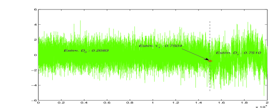
Simulations are also applied to a piecewise simulated FARIMA(0,$d_{j}$,0) processes and results are similar (see Table 3). The following Figure 2 represents the change point instant and its estimation for such a process with one abrupt change point.

Figure 2: Detection of the change point in piecewise FARIMA(0,$d_{j}$,0) (for the first segment $d_{0}=0.1$ ($D_{0}=0.2$) for the second $d_{1}=0.4$ ($D_{1}=0.8$))

$N=20000$, $\tau_{1}=0.75$, $D_{0}=0.2$ and $D_{1}=0.8$

$\widehat{\tau}_{1}$ $\widehat{\sigma}_{\tau_{1}}$ $\sqrt{MSE}$ $\tilde{D}_{0}$ $\widehat{\sigma}_{D_{0}}$ $\sqrt{MSE}$ $\tilde{D}_{1}$ $\widehat{\sigma}_{D_{1}}$ $\sqrt{MSE}$ 0.7540 0.0215 0.0218 0.1902 0.0489 0.0499 0.7926 0.0761 0.0764

Table 3: Estimation of $\tau_{1}$, $D_{0}$ and $D_{1}$ in the case of piecewise FARIMA(0,$d_{j}$,0) ($d_{0}=0.1$ and $d_{1}=0.4$) with one change point when $N=20000$ and $\ell=30$ ($50$ realizations)

3.2 Detection of abrupt change for piecewise Gaussian self-similar processes

Let us recall that $B^{H}=(B^{H}_{t})_{t\in\mathds{R}}$ is a fractional Brownian motion (FBM) with two parameters $H\in(0,1)$ and $\sigma^{2}>0$ when $B_{H}$ is a Gaussian process having stationary increments and such as

$$\mbox{Var}(B^{H}_{t}))=\sigma^{2}|t|^{2H}\,\,\,\,\forall t\in\mathds{R}.$$

It can be proved that $B_{H}$ is the only Gaussian self-similar process having stationary increments and its self-similar parameter is $H$ (a process $Y=(Y_{t})_{t\in E}$ is said to be a $H_{s}$-self-similar process if for all $c>0$ and for all $(t_{1},\ldots,t_{k})\in E^{k}$ where $k\in\mathds{N}^{*}$, the vector $\big{(}Y_{ct_{1}},\ldots,Y_{ct_{k}}\big{)}$ has the same distribution than the vector $c^{H_{s}}\big{(}Y_{t_{1}},\ldots,Y_{t_{k}}\big{)}$).
 
Now, $X$ will be called a piecewise fractional Brownian motion if:

• there exist two families of parameters $(H^{*}_{j})_{0\leq j\leq m}\in(0,1)^{m+1}$ and $(\sigma^{*2}_{j})_{0\leq j\leq m}\in(0,\infty)^{m+1}$;

• for all $j=0,\ldots,m$, for all $t\in\big{[}[N\tau_{j}^{*}],[N\tau_{j}^{*}]+1,\ldots,[N\tau_{j+1}^{*}]-1\big{]}$, $X_{t}=X^{(j)}_{t-[N\tau_{j}^{*}]}$ and $X^{(j)}=(X^{(j)}_{t})_{t\in\mathds{R}}$ is a FBM with parameters $H^{*}_{j}$ and $\sigma^{*2}_{j}$.

The wavelet analysis of FBM has been first studied by Flandrin (1992) and developed by Abry (1998) and Bardet (2002). Following this last paper, the mother wavelet $\psi$ is supposed to satisfy:
 
Assumption $W_{2}$: $\psi:\mathds{R}\to\mathds{R}$ is a piecewise continuous and left (or right)-differentiable in $[0,1]$, such that $|\psi^{\prime}(t^{-})|$ is Riemann integrable in $[0,1]$ with $\psi^{\prime}(t^{-})$ the left-derivative of $\psi$ in $t$, with support included in $[0,1]$ and $\int_{\mathds{R}}t^{p}\psi(t)\,dt=\int_{0}^{1}t^{p}\psi(t)\,dt=0~{}~{}\mbox{for}~{}~{}p=0,1.$
 
As in Assumption $W_{1}$, $\psi$ is supposed to be supported in $[0,1]$ but the following propositions are still true for any compactly supported wavelets. Assumption $W_{2}$ is clearly weaker than Assumption $W_{1}$ concerning the regularity of the mother wavelet. For instance, $\psi$ can be a Daubechies wavelet of order $d$ with $d\geq 3$ (the Haar wavelet, i.e. $d=2$, does not satisfy $\int_{0}^{1}t\,\psi(t)\,dt=0$). Another choice could be infinite support wavelets with compact effective support (it is such the case with Meyer or Mexican Hat wavelets) but the proof of the following property has to be completed.

Proposition 3.3

Assume that $X$ is a piecewise FBM as it is defined above and let $(X_{1},X_{2},\ldots,X_{N})$ be a sample of a path of $X$ (therefore $\delta_{N}=1$). Under Assumption $W_{2}$, if $(a_{n})_{n\in\mathds{N}}$ is such that $N/a_{N}\begin{array}[t]{c}\stackrel{{\scriptstyle}}{{\longrightarrow}}\\ {\scriptstyle N\rightarrow\infty}\end{array}\infty$ and $a_{N}\cdot N^{-1/3}\begin{array}[t]{c}\stackrel{{\scriptstyle}}{{\longrightarrow}}\\ {\scriptstyle N\rightarrow\infty}\end{array}\infty$, then limit theorems (4), (7) and (8) hold with $\alpha_{j}^{*}=2H_{j}^{*}+1$ and $\beta_{j}^{*}=\log\big{(}-\frac{\sigma_{j}^{*2}}{2}\int_{0}^{1}\int_{0}^{1}\psi(t)\psi(t^{\prime})|t-t^{\prime}|^{2H_{j}^{*}}dt\,dt^{\prime}\big{)}$ for all $j=0,1,\ldots,m$ and with $d_{pq}=GCD(r_{p}\,,\,r_{q})$ for all $(p,q)\in\{1,\ldots,\ell\}$,

$$\gamma^{(j)}_{pq}=\frac{2d_{pq}}{r_{p}^{2H_{j}^{*}+1/2}r_{q}^{2H_{j}^{*}+1/2}}\sum_{k=-\infty}^{\infty}\left(\frac{\int_{0}^{1}\int_{0}^{1}\psi(t)\psi(t^{\prime})\left|k\,d_{pq}+r_{p}t-r_{q}t^{\prime}\right|^{2H_{j}^{*}}dt\,dt^{\prime}}{\int_{0}^{1}\int_{0}^{1}\psi(t)\psi(t^{\prime})|t-t^{\prime}|^{2H_{j}^{*}}dt\,dt^{\prime}}\right)^{2}.$$

Then, Theorem 2.1 can be applied to piecewise FBM but $2(a^{\prime}-a)+1=2(\sup_{j}\alpha_{j}^{*}-\inf_{j}\alpha_{j}^{*})+1$ has to be smaller than $3$ since $a_{N}\cdot N^{-1/3}\begin{array}[t]{c}\stackrel{{\scriptstyle}}{{\longrightarrow}}\\ {\scriptstyle N\rightarrow\infty}\end{array}\infty$. Thus,

Corollary 3.4

Let $A:=\big{|}\sup_{j}H_{j}^{*}-\inf_{j}H_{j}^{*}\big{|}$. If $A<1/2$, under assumptions of Proposition 3.3 and Assumption C, for all $0<\kappa<\frac{1}{1+4A}-\frac{1}{3}$, if $a_{N}=N^{1/3+\kappa}$ and $v_{N}=N^{2/3(1-2A)-\kappa(2+4A)}$ then (15), (18), (21) and (24) hold.

Thus, the rate of convergence of $\underline{\widehat{\tau}}$ to $\underline{\tau}^{*}$ (in probability) can be $N^{2/3(1-2A)-\kappa^{\prime}}$ for $0<\kappa^{\prime}$ as small as one wants when $a_{N}=N^{1/3+\kappa^{\prime}/(2+4A)}$.
 
Remark: This result of Corollary 3.4 is quite surprising: the smaller $A$, i.e. the smaller the differences between the parameters $H_{j}$, the faster the convergence rates of estimators $\widehat{\tau}_{j}$ to $\tau_{j}^{*}$. And if the difference between two successive parameters $H_{j}$ is too large, the estimators ${\widehat{\tau}_{j}}$ do not seem to converge. Following simulations in Table 5 will exhibit this paroxysm. This induces a limitation of the estimators’ using especially for applying them to real data (for which a priori knowledge is not available about the values of $H_{j}^{*}$).
 
Estimators $\tilde{H}_{j}$ and ${\overline{H}_{j}}$ converge to the parameters $H_{j}^{*}$ following a central limit theorem with a rate of convergence $N^{1/3-\kappa/2}$ for $0<\kappa$ as small as one wants.
 
Results of simulations: The following Table 4 represent the change point and parameter estimations in the case of piecewise FBM with one abrupt change point. Estimators of the change points and parameters seem to converge since their mean square errors clearly decrease when we double the number of observations.

	$N=5000$	$N=10000$
$\tau_{1}$ 0.4 $H_{0}$ 0.4 $H_{1}$ 0.8	$\widehat{\tau}_{1}$ $\widehat{\sigma}_{\tau_{1}}$ $\sqrt{MSE}$ 0.4467 0.0701 0.0843 $\tilde{H}_{0}$ $\widehat{\sigma}_{H_{0}}$ $\sqrt{MSE}$ 0.3147 0.0404 0.0943 $\tilde{H}_{1}$ $\widehat{\sigma}_{H_{1}}$ $\sqrt{MSE}$ 0.7637 0.0534 0.0645	$\widehat{\tau}_{1}$ $\widehat{\sigma}_{\tau_{1}}$ $\sqrt{MSE}$ 0.4368 0.0319 0.0487 $\tilde{H}_{0}$ $\widehat{\sigma}_{H_{0}}$ $\sqrt{MSE}$ 0.3761 0.0452 0.0511 $\tilde{H}_{1}$ $\widehat{\sigma}_{H_{1}}$ $\sqrt{MSE}$ 0.7928 0.0329 0.0337

Table 4: Estimation of $\tau_{1}$, $H_{0}$ and $H_{1}$ in the case of piecewise FBM with one change point when $N=5000$ ($100$ realizations) and $N=10000$ ($50$ realizations)

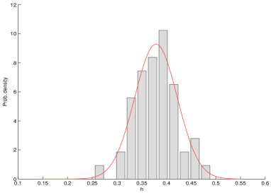
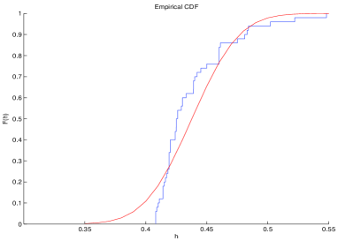
For testing if the estimated parameters follow a Gaussian distribution, Kolmogorov-Smirnov goodness-of-fit tests (in the case with $N=10000$ and $50$ replications) are applied:

1. this test for $\tilde{H}_{0}$ is accepted as well as for $\tilde{H}_{1}$ and the following Figure 3 represents the relating distribution.

2. this is not such the case for the change point estimator $\widehat{\tau}_{1}$ for which the hypothesis of a possible fit with a Gaussian distribution is rejected ($KS_{test}=0.2409$) as showed in the Figure 3 below which represents the empirical distribution function with the correspondant Gaussian cumulative distribution function.

Figure 3: Left: Modeling of sample estimations of $\tilde{H}_{0}$ with normal distribution; Right: Comparison of the generated empirical cumulative distribution for $\widehat{\tau}_{1}$ (when N=10000) and the theoretical normal distribution.

From the following example in Table 5, we remark that the estimated parameters seem to be non convergent when the difference between the parameters $H_{j}$ is too large.

$N=5000$, $\tau_{1}=0.6$, $H_{0}=0.1$ and $H_{1}=0.9$

$\widehat{\tau}_{1}$ $\widehat{\sigma}_{\tau_{1}}$ $\sqrt{MSE}$ $\tilde{H}_{0}$ $\widehat{\sigma}_{H_{0}}$ $\sqrt{MSE}$ $\tilde{H}_{1}$ $\widehat{\sigma}_{H_{1}}$ $\sqrt{MSE}$ 0.5950 0.1866 0.1866 -0.1335 0.0226 0.2346 0.6268 0.4061 0.4894

Table 5: Estimation of $\tau_{1}$, $H_{0}$ and $H_{1}$ (when $H_{1}-H_{0}=0.8>1/2$) in the case of piecewise FBM with one change point when $N=5000$ (50 realizations)

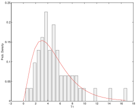
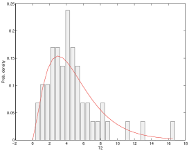
Simulations for goodness-of-fit tests $T^{(j)}$ provide the following results: when $N=5000$, the drawn distributions of the computed test statistics (see Figure 4) exhibit a Khi-square distributed values ($\chi^{2}(5)$ since $\ell=7$) and $95\%$ of the $100$ of the values of $T^{(0)}$ and $T^{(1)}$ do not exceed $\chi^{2}_{95\%}(5)=11.0705$. These results are also validated with Kolmogorov-Smirnov tests.

Figure 4: Testing for $\chi^{2}(5)$ distribution in the first detected zone (left) and the second detected zone (right) ($50$ realizations when $N=5000$)

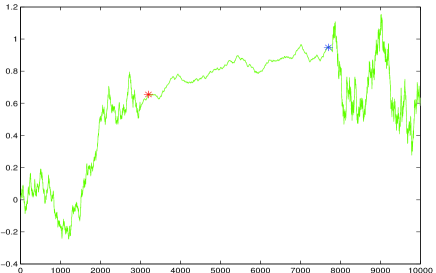
The results below in Table 6 are obtained with piecewise fractional Brownian motion when two change points are considered. As previously, both the $KS_{test}$ tests for deciding whether or not samples of both estimated change points is consistent with Gaussian distributions are rejected. However, such $KS_{test}$ tests are accepted for $\tilde{H}_{j}$ samples. A graphical representation of the change point detection method applied to a piecewise FBM is given in Figure 5.

	$N=5000$	$N=10000$
$\tau_{1}$ 0.3 $\tau_{2}$ 0.78 $H_{0}$ 0.6 $H_{1}$ 0.8 $H_{2}$ 0.5	$\widehat{\tau}_{1}$ $\widehat{\sigma}_{\tau_{1}}$ $\sqrt{MSE}$ 0.3465 0.1212 0.1298 $\widehat{\tau}_{2}$ $\widehat{\sigma}_{\tau_{2}}$ $\sqrt{MSE}$ 0.7942 0.1322 0.1330 $\tilde{H}_{0}$ $\widehat{\sigma}_{H_{0}}$ $\sqrt{MSE}$ 0.5578 0.0595 0.0730 $\tilde{H}_{1}$ $\widehat{\sigma}_{H_{1}}$ $\sqrt{MSE}$ 0.7272 0.0837 0.1110 $\tilde{H}_{2}$ $\widehat{\sigma}_{H_{2}}$ $\sqrt{MSE}$ 0.4395 0.0643 0.0883	$\widehat{\tau}_{1}$ $\widehat{\sigma}_{\tau_{1}}$ $\sqrt{MSE}$ 0.3086 0.0893 0.0897 $\widehat{\tau}_{2}$ $\widehat{\sigma}_{\tau_{2}}$ $\sqrt{MSE}$ 0.7669 0.0675 0.0687 $\tilde{H}_{0}$ $\widehat{\sigma}_{H_{0}}$ $\sqrt{MSE}$ 0.5597 0.0449 0.0604 $\tilde{H}_{1}$ $\widehat{\sigma}_{H_{1}}$ $\sqrt{MSE}$ 0.7633 0.0813 0.0892 $\tilde{H}_{2}$ $\widehat{\sigma}_{H_{2}}$ $\sqrt{MSE}$ 0.4993 0.0780 0.0780

Table 6: Estimation of $\tau_{1}$, $\tau_{2}$, $H_{0}$, $H_{1}$ and $H_{2}$ in the case of piecewise FBM with two change points when $N=5000$ and $N=10000$ (50 realizations)

Figure 5: (left)Detection of the change point in piecewice FBM($H_{j}$) ($\tau_{1}=0.3$, $\tau_{2}=0.78$, $H_{0}=0.6$, $H_{1}=0.8$ and $H_{2}=0.5$). The change points estimators are $\widehat{\tau}_{1}=0.32$ and $\widehat{\tau}_{2}=0.77$. (right) Representation of log-log regression of the variance of wavelet coefficients on the chosen scales for the three segments ($\tilde{H}_{0}=0.5608$ (*), $\tilde{H}_{1}=0.7814$ ($\lhd$) and $\tilde{H}_{2}=0.4751$ (o))

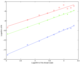
The distribution of the test statistics $T^{(0)}$, $T^{(1)}$ and $T^{(2)}$ (in this case $\ell=10$, $N=10000$ and 50 realizations) are compared with a Chi-squared-distribution with eight degrees of freedom. The goodness-of-fit Kolmogorov-Smirnov test for $T^{(j)}$ to the $\chi^{2}(8)$-distribution is accepted (with $p=0.4073$ for the sample of $T^{(0)}$, $p=0.2823$ for $T^{(1)}$ and $p=0.0619$ for $T^{(2)}$).

3.3 Detection of abrupt change for piecewise locally fractional Gaussian processes

In this section, a continuous-time process $X$ is supposed to model data. Therefore assume that $(X_{\delta_{N}},X_{2\delta_{N}},\ldots,X_{N\,\delta_{N}})$ is known, with $\delta_{N}\begin{array}[t]{c}\stackrel{{\scriptstyle}}{{\longrightarrow}}\\ {\scriptstyle N\rightarrow\infty}\end{array}0$ and $N\,\delta_{N}\begin{array}[t]{c}\stackrel{{\scriptstyle}}{{\longrightarrow}}\\ {\scriptstyle N\rightarrow\infty}\end{array}\infty$. A piecewise locally fractional Gaussian process $X=(X_{t})_{t\in\mathds{R}_{+}}$ is defined by

$$X_{t}:=\int_{\mathds{R}}\frac{e^{it\xi}-1}{\rho_{j}(\xi)}\widehat{W}(d\xi)~{}~{}\mbox{for}~{}~{}t\in[\tau_{j}^{*}N\,\delta_{N}\,,\,\tau_{j+1}^{*}N\,\delta_{N})$$ (25)

where the functions $\rho_{j}:\mathds{R}\to[0,\infty)$ are even Borelian functions such that for all $j=0,1,\ldots,m$,:

• $\displaystyle\rho_{j}(\xi)=\frac{1}{\sigma^{*}_{j}}\,|\xi|^{H^{*}_{j}+{1/2}}~{}~{}\mbox{for}~{}~{}|\xi|\in[f_{min}\,,\,f_{max}]~{}~{}\mbox{with}~{}~{}H^{*}_{j}\in\mathds{R},~{}\sigma^{*}_{j}>0$;

• $\displaystyle\int_{\mathds{R}}\left(1\wedge|\xi|^{2}\right)\frac{1}{\rho_{j}^{2}(\xi)}\,d\xi<\infty$

and $W(dx)$ is a Brownian measure and $\widehat{W}(d\xi)$ its Fourier transform in the distribution meaning. Remark that parameters $H_{j}^{*}$, called local-fractality parameters, can be supposed to be included in $\mathds{R}$ instead the usual interval $(0,1)$. Here $0<f_{min}<f_{max}$ are supposed to be known parameters. Roughly speaking, a locally fractional Gaussian process is nearly a self-similar Gaussian process for scales (or frequencies) included in a band of scales (frequencies).
 
For locally fractional Gaussian process already studied in Bardet and Bertrand (2007) and Kammoun et al. (2007), the mother wavelet is supposed to satisfy
 
Assumption $W_{3}$: $\psi:~{}\mathds{R}\mapsto\mathds{R}$ is a ${\cal C}^{\infty}(\mathds{R})$ function such that for all $m\in\mathds{N}$, $\int_{\mathds{R}}\left|t^{m}\psi(t)\right|dt<\infty$ and the Fourier transform $\widehat{\psi}$ of $\psi$ is an even function compactly supported on $[-\mu,-\lambda]\cup[\lambda,\mu]$ with $0<\lambda<\mu$.
 
These conditions are sufficiently mild and are satisfied in particular by the Lemarié-Meyer "mother" wavelet. The admissibility property, i.e. $\int_{\mathds{R}}\psi(t)dt=0$, is a consequence of the second condition and more generally, for all $m\in\mathds{N}$, $\int_{\mathds{R}}t^{m}\psi(t)dt=0.$
 
Since the function $\psi$ is not a compactly supported mother wavelet, wavelet coefficients $d_{X}(a,b)$ can not be well approximated by $e_{X}(a,b)$ when the shift $b$ is close to $0$ or $N\,\delta_{N}$. Then, a restriction $\tilde{S}^{k^{\prime}}_{k}(a_{N})$ of sample wavelet coefficient’s variance $S^{k^{\prime}}_{k}(a_{N})$ has to be defined:

$$\tilde{S}^{k^{\prime}}_{k}(a_{N}):=\frac{a_{N}}{(1-2w)k^{\prime}-k}\,\sum_{p=[(k+w(k^{\prime}-k))/a_{N}]+w}^{[(k^{\prime}-w(k^{\prime}-k))/a_{N}]-1}e_{X}^{2}(a_{N},a_{N}\,p)~{}~{}\mbox{with $0<w<1/2$}.$$

Proposition 3.5

Assume that $X$ is a piecewise locally fractional Gaussian process as it is defined above and $(X_{\delta_{N}},X_{2\delta_{N}},\ldots,X_{N\,\delta_{N}})$ is known, with $N(\delta_{N})^{2}\begin{array}[t]{c}\stackrel{{\scriptstyle}}{{\longrightarrow}}\\ {\scriptstyle N\rightarrow\infty}\end{array}0$ and $N\,\delta_{N}\begin{array}[t]{c}\stackrel{{\scriptstyle}}{{\longrightarrow}}\\ {\scriptstyle N\rightarrow\infty}\end{array}\infty$. Under Assumptions $W_{3}$ and $C$, using $\tilde{S}^{k^{\prime}}_{k}(a_{N})$ instead of $S^{k^{\prime}}_{k}(a_{N})$, if $\frac{\mu}{\lambda}<\frac{f_{max}}{f_{min}}$ and $r_{i}=\frac{f_{min}}{\lambda}+\frac{i}{\ell}\big{(}\frac{f_{max}}{\mu}-\frac{f_{min}}{\lambda}\big{)}$ for $i=1,\ldots,\ell$ with $a_{N}=1$ for all $N\in\mathds{N}$, then limit theorems (4), (7) and (8) hold with $\alpha_{j}^{*}=2H_{j}^{*}+1$ and $\beta_{j}^{*}=\log\big{(}-\frac{\sigma_{j}^{*2}}{2}\int_{\mathds{R}}\big{|}\widehat{\psi}(u)\big{|}^{2}\,|u|^{-1-2H_{j}^{*}}du\big{)}$ for all $j=0,1,\ldots,m$, for all $(p,q)\in\{1,\ldots,\ell\}$,

$$\gamma^{(j)}_{pq}=\frac{2}{(1-2w)\left(r_{p}\,r_{q}\right)^{2H_{j}^{*}}}\int_{\mathds{R}}\Big{(}\frac{\int_{\mathds{R}}\overline{\widehat{\psi}}(r_{p}\,\xi)\widehat{\psi}(r_{q}\,\xi)\,|\xi|^{-1-2H_{j}^{*}}e^{-iu\xi}d\xi}{\int_{\mathds{R}}\big{|}\widehat{\psi}(u)\big{|}^{2}\,|u|^{-1-2H_{j}^{*}}du}\Big{)}^{2}du.$$ (26)

Theorem 2.1 can be applied to a piecewise locally fractional Gaussian process without conditions on parameters $H_{j}^{*}$. Thus,

Corollary 3.6

Under assumptions of Proposition 3.5 and Assumption C, then for all $0<\kappa<\frac{1}{2}$, if $\delta_{N}=N^{-1/2-\kappa}$ and $v_{N}=N^{1/2-\kappa}$ then (15), (18), (21) and (24) hold.

Therefore the convergence rate of $\underline{\widehat{\tau}}$ to $\underline{\tau}^{*}$ (in probability) is as well close to $N^{1/2}$ as one wants. Estimators $\tilde{H}_{j}$ and ${\overline{H}_{j}}$ converge to the parameters $H_{j}^{*}$ following a central limit theorem with a rate of convergence $N^{1/4-\kappa/2}$ for $0<\kappa$ as small as one wants.

3.4 Application to heart rate’s time series

The study of the regularity of physiological data and in particular the heartbeat signals have received much attention by several authors (see for instance [24], [25] or [3]). These authors studied HR series for healthy subjects and subjects with heart disease. In [17], a piecewise locally fractional Brownian motion is studied for modeling the cumulative HR data during three typical phases (estimated from Lavielle’s algorithm) of the race (beginning, middle and end). The local-fractality parameters are estimated with wavelet analysis. The conclusions obtained are relatively close to those obtained by Peng. et al.. Indeed we remarked that the local-fractality parameter increases thought the race phases which may be explained with fatigue appearing during the last phase of the marathon. In this paper, we tray to unveil in which instants the behaviour of HR data changes. The following Table 7 presents the results for the detection of one change point.

	$\widehat{\tau}_{1}$	$\tilde{H}_{0}$	$\tilde{H}_{1}$	$T^{(0)}$	$T^{(1)}$
Ath1	0.0510	0.7880	1.2376	1.0184	1.0562
Ath2	0.4430	1.3470	1.4368	5.0644	1.5268
Ath3	0.6697	0.9542	1.2182	0.7836	0.9948
Ath4	0.4856	1.1883	1.2200	2.8966	1.2774
Ath5	0.8715	1.1512	1.3014	0.7838	0.8748
Ath6	0.5738	1.1333	1.1941	2.2042	0.7464
Ath7	0.3423	1.1905	1.1829	0.4120	1.5598
Ath8	0.8476	1.0222	1.2663	3.1704	0.5150
Ath9	0.7631	1.4388	1.3845	9.6574	0.5714

Table 7: Estimated change points $\tau_{1}$, parameters $H_{0}$, $H_{1}$ and goodness-of-fit test statistics ($T^{(0)}$ for the first zone and $T^{(1)}$ for the second one) in the case of one change point observed in HR series of different athletes.

It is noticed that the estimator of the local-fractality parameter is generally larger on the second zone than on the first although the detected change point differs from an athlete to another (only the case of Athlete 1 seems not to be relevant). This result is very interesting and confirms our conclusions in [17]. Whatever is the position of change point, the estimation of the local-fractality parameter is larger in the second segment than in the first segment (see the example of HR data recorded for one athlete in Figure 6).

Figure 6: Evolution of local-fractality parameter estimators (observed for HR series of one athlete) in the two zones when the change point varies in time.

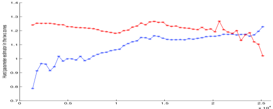
In general, the goodness-of-fit tests, with values $T^{(0)}$ and $T^{(1)}$, are less than $\chi^{2}_{95\%}(4)=9.4877$ (except $T^{(0)}$ for Ath9) when $\ell=6$. So, the HR data trajectory in the both zones seems to be correctly modeled with a stationary locally fractional Gaussian trajectory.

4 Proofs

Before establishing the proof of Theorem 2.1 an important lemma can be stated:

Lemma 4.1

Let $k\in\mathds{N}\setminus\{0,1\}$, $(\gamma_{i})_{1\leq i\leq k}\in(0,\infty)^{k}$ and $\alpha_{1}>\alpha_{2}>\cdots>\alpha_{k}$ be $k$ ordered real numbers. For $(\alpha,\beta)\in\mathds{R}^{2}$, consider the function $f_{\alpha,\beta}:x\in\mathds{R}\mapsto\mathds{R}$ such that

$$f_{\alpha,\beta}(x):=\alpha\,x+\beta-\log\Big{(}\sum_{q=1}^{k}\gamma_{q}\exp\big{(}\alpha_{q}\,x\big{)}\Big{)}~{}~{}\mbox{for}~{}x\in\mathds{R}.$$

Let $0<t_{1}<\cdots<t_{\ell}$ with $\ell\in\mathds{N}\setminus\{0,1,2\}$ and $(u_{n})_{n\in\mathds{N}}$ be a sequence of real numbers such that there exists $m\in\mathds{R}$ satisfying $u_{n}\geq m$ for all $n\in\mathds{N}$. Then there exists $C>0$ not depending on $n$ such that

$$\inf_{(\alpha,\beta)\in\mathds{R}^{2}}\sum_{i=1}^{\ell}\big{|}f_{\alpha,\beta}\big{(}\log(u_{n})+t_{i}\big{)}\big{|}^{2}\geq C\,\min\big{(}1,|u_{n}|^{2(\alpha_{2}-\alpha_{1})}\big{)}.$$

Proof of Lemma 4.1: For all $(\alpha,\beta)\in\mathds{R}^{2}$, the function $f_{\alpha,\beta}$ is a $\mathcal{C}^{\infty}(\mathds{R})$ function and

$$\frac{\partial^{2}}{\partial x^{2}}f_{\alpha,\beta}(x)=-\frac{\sum_{q=1}^{k-1}\gamma_{q}\gamma_{q+1}(\alpha_{q}-\alpha_{q+1})^{2}\exp\big{(}(\alpha_{q}+\alpha_{q+1})\,x\big{)}}{\Big{(}\sum_{q=1}^{k}\gamma_{q}\exp\big{(}\alpha_{q}\,x\big{)}\Big{)}^{2}}<0.$$

Therefore the function $f_{\alpha,\beta}$ is a concave function such that $\sup_{(\alpha,\beta)\in\mathds{R}^{2}}\frac{\partial^{2}}{\partial x^{2}}f_{\alpha,\beta}(x)<0$ (not depending on $\alpha$ and $\beta$) and for all $(\alpha,\beta)\in\mathds{R}^{2}$, $f_{\alpha,\beta}$ vanishes in $2$ points at most. Thus, since $\ell\geq 3$ and $\big{(}x+t_{i}\big{)}_{i}$ are distinct points, for all $x\in\mathds{R}$, it exists $C(x)>0$ not depending on $\alpha$ and $\beta$ such that

$$\inf_{(\alpha,\beta)\in\mathds{R}^{2}}\sum_{i=1}^{\ell}\big{|}f_{\alpha,\beta}\big{(}x+t_{i}\big{)}\big{|}^{2}\geq C(x).$$

Therefore, since for all $M\geq 0$,

$$\inf_{x\in[-M,M]}\left\{\inf_{(\alpha,\beta)\in\mathds{R}^{2}}\sum_{i=1}^{\ell}\big{|}f_{\alpha,\beta}\big{(}x+t_{i}\big{)}\big{|}^{2}\right\}\geq\inf_{x\in[-M,M]}\big{\{}C(x)\big{\}}>0.$$ (27)

Moreover, if $u_{n}\to+\infty$,

$$\log\Big{(}\sum_{q=1}^{k}\gamma_{q}\exp\big{(}\alpha_{q}\,\log(u_{n})\big{)}\Big{)} = \log\Big{(}\gamma_{1}\exp\big{(}\alpha_{1}\,\log(u_{n})\big{)}+\gamma_{2}\exp\big{(}\alpha_{2}\,\log(u_{n})\big{)}\big{(}1+o(1)\big{)}\Big{)}$$

$$= \log(\gamma_{1})+\alpha_{1}\log(u_{n})+\gamma_{2}\exp\big{(}(\alpha_{2}-\alpha_{1})\,\log(u_{n})\big{)}\big{(}1+o(1)\big{)}.$$

Thus, for $n$ large enough,

$$\frac{1}{2}\,\gamma_{2}\,u_{n}^{\alpha_{2}-\alpha_{1}}\leq\Big{|}\log\Big{(}\sum_{q=1}^{k}\gamma_{q}\exp\big{(}\alpha_{q}\,\log(u_{n})\big{)}\Big{)}-\log(\gamma_{1})+\alpha_{1}\log(u_{n})\Big{|}\leq 2\,\gamma_{2}\,u_{n}^{\alpha_{2}-\alpha_{1}}.$$ (28)

Therefore, for all $(\alpha,\beta)\in\mathds{R}^{2}$,

$$\big{|}f_{\alpha,\beta}\big{(}\log(u_{n})+t_{i}\big{)}\big{|}^{2}=\big{|}f_{\alpha_{1},\log(\gamma_{1})}\big{(}\log(u_{n})+t_{i}\big{)}\big{|}^{2}+\Big{|}(\log(\gamma_{1})-\beta)+(\alpha_{1}-\alpha)(\log(u_{n})+t_{i})\Big{|}^{2}\\ -2f_{\alpha_{1},\log(\gamma_{1})}\big{(}\log(u_{n})+t_{i}\big{)}\times\Big{(}(\log(\gamma_{1})-\beta)+(\alpha_{1}-\alpha)(\log(u_{n})+t_{i})\Big{)}.$$

Using inequalities (28), $\displaystyle\frac{1}{4}\,\gamma_{2}^{2}\,u_{n}^{2(\alpha_{2}-\alpha_{1})}\leq\big{|}f_{\alpha_{1},\log(\gamma_{1})}\big{(}\log(u_{n})+t_{i}\big{)}\big{|}^{2}\leq 4\,\gamma_{2}^{2}\,u_{n}^{2(\alpha_{2}-\alpha_{1})}$ and for all $(\alpha,\beta)\in\mathds{R}^{2}$, $\displaystyle\lim_{n\to\infty}f_{\alpha_{1},\log(\gamma_{1})}\big{(}\log(u_{n})+t_{i}\big{)}\times\Big{(}(\log(\gamma_{1})-\beta)+(\alpha_{1}-\alpha)(\log(u_{n})+t_{i})\Big{)}=0$. Then, for all $\displaystyle(\alpha,\beta)\neq(\alpha_{1},\log(\gamma_{1}))$, $\displaystyle\lim_{n\to\infty}\big{|}f_{\alpha,\beta}\big{(}\log(u_{n})+t_{i}\big{)}\big{|}^{2}=\infty$. Consequently, for $n$ large enough,

$$\inf_{(\alpha,\beta)\in\mathds{R}^{2}}\sum_{i=1}^{\ell}\big{|}f_{\alpha,\beta}\big{(}\log(u_{n})+t_{i}\big{)}\big{|}^{2} \geq \frac{1}{2}\,\sum_{i=1}^{\ell}\big{|}f_{\alpha_{1},\log(\gamma_{1})}\big{(}\log(u_{n})+t_{i}\big{)}\big{|}^{2}$$

$$\geq \frac{1}{8}\,\gamma_{2}^{2}\,\sum_{i=1}^{\ell}(u_{n}+t_{i})^{2(\alpha_{2}-\alpha_{1})}$$

$$\geq C\,u_{n}^{2(\alpha_{2}-\alpha_{1})},$$

which combined with (27) achieves the proof. $\Box$

Proof of Theorem 2.1: Let $\displaystyle w_{N}=\frac{N\delta_{N}}{v_{N}}$, $k_{j}^{*}=[N\delta_{N}\tau_{j}^{*}]$ for $j=1,\ldots,m$ and

$$V_{\eta\,w_{N}}=\{(k_{j})_{1\leq j\leq m},~{}\max_{j\in{1,\ldots,m}}|k_{j}-k^{*}_{j}|\geq\eta\,w_{N}\}.$$

Then, for $N\delta_{N}$ large enough,

$$\mathds{P}\Big{(}\frac{N\delta_{N}}{w_{N}}\,\|\underline{\tau}^{*}-\underline{\widehat{\tau}}\|_{m}\geq\eta\Big{)} \simeq \mathds{P}(\max_{j\in{1,\ldots,m}}|\widehat{k}_{j}-k^{*}_{j}|\geq\eta\,w_{N})$$ (29)

$$= \mathds{P}\Big{(}\min_{(k_{j})_{1\leq j\leq m}\in V_{\eta\,w_{N}}}G_{N}\big{(}(k_{j})_{1\leq j\leq m}\big{)}\leq\min_{(k_{j})_{1\leq j\leq m}\notin V_{\eta\,w_{N}}}G_{N}\big{(}(k_{j})_{1\leq j\leq m}\big{)}\Big{)}$$

$$\leq \mathds{P}\Big{(}\min_{(k_{j})_{1\leq j\leq m}\in V_{\eta\,w_{N}}}G_{N}\big{(}(k_{j})_{1\leq j\leq m}\big{)}\leq G_{N}\big{(}(k_{j}^{*})_{1\leq j\leq m}\big{)}\Big{)}.$$

For $j=\{0,\ldots,m\}$ and $0=k_{0}<k_{1}<\ldots<k_{m}<k_{m+1}=N\delta_{N}$, let

• $Y_{k_{j}}^{k_{j+1}}:=\big{(}\log\big{(}S^{k_{j+1}}_{k_{j}}(r_{i}\cdot a_{N})\big{)}\big{)}_{1\leq i\leq\ell}$,

• $\Theta^{k_{j+1}}_{k_{j}}=\left(\begin{array}[]{c}\alpha_{j}\\ \log\beta_{j}\\ \end{array}\right)$,    $\widehat{\Theta}^{k_{j+1}}_{k_{j}}=\left(\begin{array}[]{c}\widehat{\alpha}_{j}\\ \log\widehat{\beta}_{j}\\ \end{array}\right)$   and  $\Theta^{*}_{j}=\left(\begin{array}[]{c}\alpha^{*}_{j}\\ \log\beta^{*}_{j}\\ \end{array}\right)$.

1/ Using these notations, $\displaystyle{G_{N}\big{(}(k_{j})_{1\leq j\leq m}\big{)}=\sum_{j=0}^{m}\parallel Y^{k_{j+1}}_{k_{j}}-L_{a_{N}}\cdot\widehat{\Theta}^{k_{j+1}}_{k_{j}}\parallel^{2}}$, where $\parallel\cdot\parallel$ denotes the usual Euclidean norm in $\mathds{R}^{\ell}$. Then, with $I_{\ell}$ the $(\ell\times\ell)$-identity matrix

$$G_{N}\big{(}(k_{j}^{*})_{1\leq j\leq m}\big{)} = \sum_{j=0}^{m}\parallel Y^{k^{*}_{j+1}}_{k^{*}_{j}}-L_{a_{N}}\cdot\Theta^{*}_{j}\parallel^{2}$$

$$= \sum_{j=0}^{m}\Big{\|}(I_{\ell}-P_{L_{a_{N}}})\cdot Y_{k_{j}^{*}}^{k_{j+1}^{*}}\Big{\|}^{2}\mbox{~{}~{}~{}~{}~{}~{}~{}~{}~{}~{}~{}~{}~{}with $P_{L_{a_{N}}}=L_{a_{N}}\cdot(L_{a_{N}}^{\prime}\cdot L_{a_{N}})^{-1}\cdot L_{a_{N}}^{\prime}$}$$

$$= \sum_{j=0}^{m}\frac{a_{N}}{k^{*}_{j+1}-k^{*}_{j}}\Big{\|}(I_{\ell}-P_{L_{a_{N}}})\cdot\big{(}\varepsilon_{i}^{(N)}(k^{*}_{j},k^{*}_{j+1})\big{)}_{1\leq i\leq\ell}\Big{\|}^{2}~{}~{}~{}~{}~{}~{}~{}~{}~{}~{}~{}~{}~{}~{}\mbox{from (\ref{TLClogS})}$$

$$\leq \frac{1}{\min_{0\leq j\leq m}(\tau^{*}_{j+1}-\tau^{*}_{j})}\cdot\frac{a_{N}}{N\,\delta_{N}}\,\sum_{j=0}^{m}\Big{\|}\big{(}\varepsilon_{i}^{(N)}(k^{*}_{j},k^{*}_{j+1})\big{)}_{1\leq i\leq\ell}\Big{\|}^{2}.$$

Now, using the limit theorem (7), $\displaystyle\Big{\|}\big{(}\varepsilon_{i}^{(N)}(k^{*}_{j},k^{*}_{j+1})\big{)}_{1\leq i\leq\ell}\Big{\|}^{2}\begin{array}[t]{c}\stackrel{{\scriptstyle{\mathcal{L}}}}{{\longrightarrow}}\\ {\scriptstyle N\rightarrow\infty}\end{array}\Big{\|}\mathcal{N}(0,\Gamma(r_{1},\ldots,r_{\ell}))\Big{\|}^{2}$ since $k^{*}_{j+1}-k^{*}_{j}\sim N\delta_{N}(\tau_{i+1}^{*}-\tau_{i}^{*})\begin{array}[t]{c}\stackrel{{\scriptstyle}}{{\longrightarrow}}\\ {\scriptstyle N\rightarrow\infty}\end{array}\infty$, and thus

$$G_{N}\big{(}(k_{j}^{*})_{1\leq j\leq m}\big{)}=O_{P}\Big{(}\frac{a_{N}}{N\,\delta_{N}}\Big{)},$$ (30)

where $\xi_{N}=O_{P}(\psi_{N})$ as $N\to\infty$ is written, if for all $\rho>0$, there exists $c>0$, such as $P\Big{(}|\xi_{N}|\leq c\cdot\psi_{N}\Big{)}\geq 1-\rho$ for all sufficiently large $N$.
 
2/ Now, set $(k_{j})_{1\leq j\leq m}\in V_{\eta\,w_{N}}$. Therefore, for $N$ and $N\,\delta_{N}$ large enough, there exists $j_{0}\in\{1,\ldots,m\}$ and $(j_{1},j_{2})\in\{1,\ldots,m\}^{2}$ with $j_{1}\leq j_{2}$ such that $k_{j_{0}}\leq k^{*}_{j_{1}}-\eta\,w_{N}$ and $k_{j_{0}+1}\geq k^{*}_{j_{2}}+\eta\,w_{N}$. Thus,

$$G_{N}\big{(}(k_{j})_{1\leq j\leq m}\big{)}\geq\big{\|}Y_{k_{j_{0}}}^{k_{{j_{0}}+1}}-L_{a_{N}}\widehat{\Theta}_{k_{j_{0}}}^{k_{{j_{0}}+1}}\big{\|}^{2}.$$

Let $\Omega^{*}:=\big{(}\Omega^{*}_{i}\big{)}_{1\leq i\leq\ell}$ be the vector such that

$$\Omega^{*}_{i} := {\frac{k^{*}_{j_{1}}-k_{j_{0}}}{k_{{j_{0}}+1}-k_{j_{0}}}}\,\beta^{*}_{j_{1}-1}\exp\big{(}\alpha^{*}_{j_{1}-1}\log(r_{i}\,a_{N})\big{)}+\sum_{j=j_{1}}^{j_{2}-1}{\frac{k^{*}_{j+1}-k^{*}_{j_{1}}}{k_{{j_{0}}+1}-k_{j_{0}}}}\beta^{*}_{j}\exp\big{(}\alpha^{*}_{j}\log(r_{i}\,a_{N})\big{)}$$

$$\hskip 199.16928pt+{\frac{k_{j_{0}+1}-k^{*}_{j_{2}}}{k_{{j_{0}}+1}-k_{j_{0}}}}\beta^{*}_{j_{2}}\exp\big{(}\alpha^{*}_{j_{2}}\log(r_{i}\,a_{N})\big{)}.$$

Then,

$$G_{N}\big{(}(k_{j})_{1\leq j\leq m}\big{)}\geq\parallel Y_{k_{j_{0}}}^{k_{{j_{0}}+1}}-\big{(}\log\Omega^{*}_{i}\big{)}_{1\leq i\leq\ell}\parallel^{2}+\parallel\big{(}\log\Omega^{*}_{i}\big{)}_{1\leq i\leq\ell}-L_{a_{N}}\cdot\widehat{\Theta}_{k_{j_{0}}}^{k_{{j_{0}}+1}}\parallel^{2}+2\,Q,$$ (31)

with $Q=\big{(}Y_{k_{j_{0}}}^{k_{{j_{0}}+1}}-\big{(}\log\Omega^{*}_{i}\big{)}_{1\leq i\leq\ell}\big{)}^{\prime}\cdot\big{(}\big{(}\log\Omega^{*}_{i}\big{)}_{1\leq i\leq\ell}-L_{a_{N}}\cdot\widehat{\Theta}_{k_{j_{0}}}^{k_{{j_{0}}+1}}\big{)}.$
In the one hand, with $S^{k^{\prime}}_{k}(\cdot)$ defined in (3),

$$S_{k_{j_{0}}}^{k_{{j_{0}}+1}}(r_{i}\,a_{N})={\frac{k^{*}_{j_{1}}-k_{j_{0}}}{k_{{j_{0}}+1}-k_{j_{0}}}}\,S_{k_{j_{0}}}^{k^{*}_{j_{1}}}(r_{i}\,a_{N})+\sum_{j=j_{1}}^{j_{2}-1}{\frac{k^{*}_{j+1}-k^{*}_{j_{1}}}{k_{{j_{0}}+1}-k_{j_{0}}}}S_{k^{*}_{j}}^{k^{*}_{j+1}}(r_{i}\,a_{N})+{\frac{k_{j_{0}+1}-k^{*}_{j_{2}}}{k_{{j_{0}}+1}-k_{j_{0}}}}S_{k_{j_{2}}}^{k^{*}_{j_{0}+1}}(r_{i}\,a_{N}).$$

Using the central limit theorems (8), for $N$ and $N\,\delta_{N}$ large enough,

$$\mathds{E}\Big{[}\big{(}S_{k_{j_{0}}}^{k_{{j_{0}}+1}}(r_{i}\,a_{N})-\Omega^{*}_{i}\big{)}^{2}\Big{]} \leq m\,\left(\Big{(}{\frac{k^{*}_{j_{1}}-k_{j_{0}}}{k_{{j_{0}}+1}-k_{j_{0}}}}\Big{)}^{2}\,\mathds{E}\Big{[}\big{(}S_{k_{j_{0}}}^{k^{*}_{j_{1}}}(r_{i}\,a_{N})-\beta^{*}_{j_{1}-1}\big{(}r_{i}\,a_{N}\big{)}^{\alpha^{*}_{j_{1}-1}}\big{)}^{2}\Big{]}\right.$$

$$+\sum_{j=j_{1}}^{j_{2}-1}\Big{(}{\frac{k^{*}_{j+1}-k^{*}_{j_{1}}}{k_{{j_{0}}+1}-k_{j_{0}}}}\Big{)}^{2}\,\mathds{E}\Big{[}\big{(}S_{k^{*}_{j}}^{k^{*}_{j+1}}(r_{i}\,a_{N})-\beta^{*}_{j}\big{(}r_{i}\,a_{N}\big{)}^{\alpha^{*}_{j}}\big{)}^{2}\Big{]}$$

$$\left.+\Big{(}{\frac{k_{j_{0}+1}-k^{*}_{j_{2}}}{k_{{j_{0}}+1}-k_{j_{0}}}}\Big{)}^{2}\,\mathds{E}\Big{[}\big{(}S_{k_{j_{2}}}^{k^{*}_{j_{0}+1}}(r_{i}\,a_{N})-\beta^{*}_{j_{2}}\big{(}r_{i}\,a_{N}\big{)}^{\alpha^{*}_{j_{2}}}\big{)}^{2}\Big{]}\right)$$

$$\Longrightarrow~{}~{}~{}\mathds{E}\Big{[}\big{(}\frac{S_{k_{j_{0}}}^{k_{{j_{0}}+1}}(r_{i}\,a_{N})}{\Omega^{*}_{i}}-1\big{)}^{2}\Big{]} \leq \frac{m\,\gamma^{2}}{\Omega^{*}_{i}}\,{a_{N}}\,\,\Big{(}\frac{1}{k^{*}_{j_{1}}-k_{j_{0}}}+\sum_{j=j_{1}}^{j_{2}-1}\frac{1}{k^{*}_{j+1}-k^{*}_{j_{1}}}+\frac{1}{k^{*}_{j_{0}+1}-k_{j^{*}_{2}}}\Big{)}$$

$$\leq C\,\frac{a_{N}}{\eta\,w_{N}},$$

with $\gamma^{2}=\max_{i,j}\{\gamma_{ii}^{(j)}\}$ (where $(\gamma_{pq}^{(j)})$ is the asymptotic covariance of vector $\varepsilon_{p}^{(N)}(k,k^{\prime})$ and $\varepsilon_{q}^{(N)}(k,k^{\prime})$) and $C>0$ not depending on $N$. Therefore, for $N$ large enough, for all $i=1,\ldots,\ell$,

$$\mathds{E}\Big{[}\big{(}\log(S_{k_{j_{0}}}^{k_{{j_{0}}+1}}(r_{i}\,a_{N}))-\log(\Omega^{*}_{i})\big{)}^{2}\Big{]}\leq 2\,C\,\frac{a_{N}}{\eta\,w_{N}}.$$

Then we deduce with Markov Inequality that

$$\parallel Y_{k_{j_{0}}}^{k_{{j_{0}}+1}}-\big{(}\log\Omega^{*}_{i}\big{)}_{1\leq i\leq\ell}\parallel^{2}=O_{P}\Big{(}\frac{a_{N}}{\eta\,w_{N}}\Big{)}.$$ (32)

>From the other hand,

$$\parallel\big{(}\log\Omega^{*}_{i}\big{)}_{1\leq i\leq\ell}-L_{a_{N}}\cdot\widehat{\Theta}_{k_{j_{0}}}^{k_{{j_{0}}+1}}\parallel^{2}=\sum_{i=1}^{\ell}\Big{(}\big{(}\widehat{\alpha}_{j_{0}}\log(r_{i}\,a_{N})+\log\widehat{\beta}_{j_{0}}\big{)}-\log\Omega^{*}_{i}\Big{)}^{2}.$$

Define $\displaystyle\gamma_{1}:={\frac{k^{*}_{j_{1}-1}-k_{j_{0}}}{k_{{j_{0}}+1}-k_{j_{0}}}}\cdot\beta^{*}_{j_{1}-1}$, for all $p\in\{0,1,\ldots,j_{2}-j_{1}-1\}$, $\displaystyle\gamma_{p}:={\frac{k^{*}_{j_{1}+p}-k^{*}_{j_{1}+p-1}}{k_{{j_{0}}+1}-k_{j_{0}}}}\cdot\beta^{*}_{j_{1}+p-1}$ and $\displaystyle\gamma_{j_{2}-j_{1}+1}:={\frac{k_{j_{0}+1}-k^{*}_{j_{2}}}{k_{{j_{0}}+1}-k_{j_{0}}}}\cdot\beta^{*}_{j_{2}}$. Then, using Lemma 4.1, one obtains

$$\inf_{\alpha,\beta}\Big{\{}\sum_{i=1}^{\ell}\Big{(}\big{(}\alpha\log(r_{i}\,a_{N})+\log\beta\big{)}-\log\Omega^{*}_{i}\Big{)}^{2}\Big{\}}\geq C\,\min\big{(}1_{,},\,|a_{N}|^{2(\alpha^{*}_{(2)}-\alpha^{*}_{(1)})}\big{)},$$

where $C>0$ and $\alpha^{*}_{(1)}=\max_{j=j_{1}-1,\ldots,j_{2}}\alpha_{j}^{*}$, $\alpha^{*}_{(2)}=\max_{j=j_{1}-1,\ldots,j_{2},~{}j\neq(1)}\alpha_{j}^{*}$. As a consequence, for satisfying all possible cases of $j_{0}$, $j_{1}$ and $j_{2}$, one obtains

$$\parallel\big{(}\log\Omega^{*}_{i}\big{)}_{1\leq i\leq\ell}-L_{a_{N}}\cdot\widehat{\Theta}_{k_{j_{0}}}^{k_{{j_{0}}+1}}\parallel^{2}\geq C\,|a_{N}|^{2(\min_{i}\alpha^{*}_{i}-\max_{i}\alpha^{*}_{i})}.$$ (33)

Finally, using Cauchy-Schwarz Inequality,

$$Q \leq \Big{(}\big{\|}Y_{k_{j_{0}}}^{k_{{j_{0}}+1}}-\big{(}\log\Omega^{*}_{i}\big{)}_{1\leq i\leq\ell}\big{\|}^{2}\cdot\big{\|}\big{(}\log\Omega^{*}_{i}\big{)}_{1\leq i\leq\ell}-L_{a_{N}}\cdot\widehat{\Theta}_{k_{j_{0}}}^{k_{{j_{0}}+1}}\big{|}^{2}\Big{)}^{1/2}$$

Therefore, using (32) and (33), since under assumptions of Theorem 2.1,

$$\frac{a_{N}}{\eta\,w_{N}}=o\Big{(}|a_{N}|^{2(\min_{i}\alpha^{*}_{i}-\max_{i}\alpha^{*}_{i})}\Big{)},$$

then

$$Q=o_{P}\Big{(}\parallel\big{(}\log\Omega^{*}_{i}\big{)}_{1\leq i\leq\ell}-L_{a_{N}}\cdot\widehat{\Theta}_{k_{j_{0}}}^{k_{{j_{0}}+1}}\parallel^{2}\Big{)}.$$ (34)

We deduce from relations (31), (32), (33) and (34) that

$$\mathds{P}\Big{(}\min_{(k_{j})_{1\leq j\leq m}\in V_{\eta\,w_{N}}}G_{N}\big{(}(k_{j})_{1\leq j\leq m}\big{)}\geq\frac{C}{2}\,|a_{N}|^{2(\min_{i}\alpha^{*}_{i}-\max_{i}\alpha^{*}_{i})}\Big{)}\begin{array}[t]{c}\stackrel{{\scriptstyle}}{{\longrightarrow}}\\ {\scriptstyle N\rightarrow\infty}\end{array}1.$$

$\hfill\Box$

Proof of Theorem 2.2: From Theorem 2.1, it is clear that

$$\mathds{P}\big{(}[\tilde{k}_{j},\tilde{k}_{j}^{\prime}]\subset[k_{j}^{*},k^{*}_{j+1}]\big{)}\begin{array}[t]{c}\stackrel{{\scriptstyle}}{{\longrightarrow}}\\ {\scriptstyle N\rightarrow\infty}\end{array}1~{}~{}\mbox{and}~{}~{}\frac{\tilde{k}_{j}^{\prime}-\tilde{k}_{j}}{N\delta_{N}(\tau_{j+1}^{*}-\tau_{j}^{*})}\begin{array}[t]{c}\stackrel{{\scriptstyle{\mathcal{P}}}}{{\longrightarrow}}\\ {\scriptstyle N\rightarrow\infty}\end{array}1.$$ (39)

Now, for $j=0,\ldots,m$, $(x_{i})_{1\leq i\leq\ell}\in\mathds{R}^{\ell}$ and $0<\varepsilon<1$, let $A_{j}$ and $B_{j}$ be the events such that

$$A_{j}:=\Big{\{}[\tilde{k}_{j},\tilde{k}_{j}^{\prime}]\subset[k_{j}^{*},k^{*}_{j+1}]\Big{\}}\bigcap\left\{\Big{|}\frac{\tilde{k}_{j}^{\prime}-\tilde{k}_{j}}{N\delta_{N}(\tau_{j+1}^{*}-\tau_{j}^{*})}-1\Big{|}\leq\varepsilon\right\}\\ ~{}~{}\mbox{and}~{}~{}B_{j}:=\left\{\sqrt{\frac{\tilde{k}_{j}^{\prime}-\tilde{k}_{j}}{a_{N}}}\Big{(}Y_{\tilde{k}_{j}}^{\tilde{k}_{j}^{\prime}}-L_{a_{N}}\cdot\Theta^{*}_{j}\Big{)}\in\prod_{i=1}^{\ell}(-\infty,x_{i}]\right\}$$

First, it is obvious that

$$\mathds{P}(A_{j})\mathds{P}(B_{j}\mid A_{j})\leq\mathds{P}(B_{j})\leq\mathds{P}(B_{j}\mid A_{j})+1-\mathds{P}(A_{j}).$$ (40)

Moreover, from (4),

$$\mathds{P}(B_{j}\mid A_{j}) = \mathds{P}\Big{(}\big{(}\varepsilon_{i}^{(N)}(\tilde{k}_{j},\tilde{k}_{j}^{\prime})\big{)}_{1\leq i\leq\ell}\in\prod_{i=1}^{\ell}(-\infty,x_{i}]\mid A_{j}\Big{)}$$

$$\begin{array}[t]{c}\stackrel{{\scriptstyle}}{{\longrightarrow}}\\ {\scriptstyle N\rightarrow\infty}\end{array} \mathds{P}\Big{(}\mathcal{N}\big{(}0,\Gamma^{(j)}(\alpha_{j}^{*},r_{1},\ldots,r_{\ell})\big{)}\in\prod_{i=1}^{\ell}(-\infty,x_{i}]\Big{)}.$$

Using (39), it is straightforward that $\mathds{P}(A_{j})\begin{array}[t]{c}\stackrel{{\scriptstyle}}{{\longrightarrow}}\\ {\scriptstyle N\rightarrow\infty}\end{array}1$. Consequently,

$$\mathds{P}(B_{j})\begin{array}[t]{c}\stackrel{{\scriptstyle}}{{\longrightarrow}}\\ {\scriptstyle N\rightarrow\infty}\end{array}\mathds{P}\Big{(}\mathcal{N}\big{(}0,\Gamma^{(j)}(\alpha_{j}^{*},r_{1},\ldots,r_{\ell})\big{)}\in\prod_{i=1}^{\ell}(-\infty,x_{i}]\Big{)}$$

and therefore $\displaystyle\sqrt{\frac{\tilde{k}_{j}^{\prime}-\tilde{k}_{j}}{a_{N}}}\Big{(}Y_{\tilde{k}_{j}}^{\tilde{k}_{j}^{\prime}}-L_{a_{N}}\cdot\Theta^{*}_{j}\Big{)}\begin{array}[t]{c}\stackrel{{\scriptstyle{\mathcal{L}}}}{{\longrightarrow}}\\ {\scriptstyle N\rightarrow\infty}\end{array}\mathcal{N}\big{(}0,\Gamma^{(j)}(\alpha_{j}^{*},r_{1},\ldots,r_{\ell})\big{)}$. Now using again (39) and Slutsky’s Lemma one deduces

$$\sqrt{\frac{\delta_{N}\,\big{(}N(\tau_{j+1}^{*}-\tau_{j}^{*})\big{)}}{a_{N}}}\Big{(}Y_{\tilde{k}_{j}}^{\tilde{k}_{j}^{\prime}}-L_{a_{N}}\cdot\Theta^{*}_{j}\Big{)}\begin{array}[t]{c}\stackrel{{\scriptstyle{\mathcal{L}}}}{{\longrightarrow}}\\ {\scriptstyle N\rightarrow\infty}\end{array}\mathcal{N}\big{(}0,\Gamma^{(j)}(\alpha_{j}^{*},r_{1},\ldots,r_{\ell})\big{)}.$$

Using the expression of $\tilde{\Theta}_{j}$ as a linear application of $Y_{\tilde{k}_{j}}^{\tilde{k}_{j}^{\prime}}$, this achieves the proof of Theorem 2.2. $\hfill\Box$

Bibliography

- [1] Abry P., Flandrin P., Taqqu M.S., Veitch D., Self-similarity and long-range dependence through the wavelet lens, In P. Doukhan, G. Oppenheim and M.S. Taqqu editors, Long-range Dependence: Theory and Applications, Birkhäuser, 2003.
- [2] Abry P., Veitch D., Flandrin P., Long-range dependent: revisiting aggregation with wavelets J. Time Ser. Anal., Vol. 19, 253-266, 1998.
- [3] Absil P.A., Sepulchre R., Bilge A., Gérard P., Nonlinear analysis of cardiac rhythm fluctuations using DFA method, J. Physica A : Statistical mechanics and its applications, 235-244, 1999.
- [4] Bai J. Least squares estimation of a shift in linear processes. J. of Time Series Anal. 5, p. 453-472, 1998.
- [5] Bai J., Perron P. Estimating and testing linear models with multiple structural changes. Econometrica 66, p. 47-78, 1998.
- [6] Bardet J.M., Statistical Study of the Wavelet Analysis of Fractional Brownian Motion, IEEE Trans. Inf. Theory, Vol. 48, No. 4, 991-999, 2002.
- [7] Bardet J.M., Bertrand P., Identification of the multiscale fractional Brownian motion with biomechanical applications, Journal of Time Series Analysis, 1-52, 2007.
- [8] Bardet J.M., Bibi H., Jouini A., Adaptative wavelet based estimator of the memory parameter for stationary Gaussian processes, To appear in Bernouilli, 2007.
- [9] Bardet J.M., Lang G., Moulines E., Soulier P., Wavelet estimator of long range-dependant processes, Statist. Infer. Stochast. Processes, Vol. 3, 85-99, 2000.
- [10] Beran J., Terrin N., Testing for a change of the long-memory parameter, Biometrika, 83, 627-638, 1996.
- [11] Doukhan, P., G. Openheim, G. and Taqqu, M.S. (Editors), Theory and applications of long-range dependence, Birkhäuser, Boston, 2003.
- [12] Flandrin P., Wavelet analysis and synthesis of fractional Brownian motion. IEEE Trans. on Inform. Theory, 38, p. 910-917, 1992.
- [13] Giraitis L., Leipus R., Surgailis D., The change-point problem for dependent observations, Journal of Statistical Planning and Inference, 53, 297-310, 1996.
- [14] Giraitis L., Robinson P., Samarov A., Rate optimal semi-parametric estimation of the memory parameter of the Gaussian time series with long range dependence, J. Time Ser. Anal., 18, 49-61, 1997.
- [15] Horváth L., Change-Point Detection in Long-Memory Processes, Journal of Multivariate Analysis, 78, 218-134, 2001.
- [16] Horváth L., Shao Q.M., Limit theorems for quadratic forms with applications to Whittle’s estimate, The Annals of Applied Probability, 9, 146-187, 1999.
- [17] Kammoun I., Billat V., Bardet J.M., Comparison of DFA vs wavelet analysis for estimation of regularity of HR series during the marathon, Preprint SAMOS, 2007.
- [18] Kokoszka P.S., Leipus R., Detection and estimation of changes in regime, In P. Doukhan, G. Oppenheim and M.S. Taqqu editors, Long-range Dependence: Theory and Applications, Birkhäuser, 325-337, 2003.
- [19] Lavielle M., Detection of multiple changes in a sequence of random variables, Stoch. Process Appl, 79-102, 1999.
- [20] Lavielle, M. and Moulines, E., Least-squares estimation of an unknown number of shifts in a time series, J. of Time Series Anal., 33-59, 2000.
- [21] Lavielle M., Teyssière G. Detecting Multiple Change-Points in Multivariate Time Series, Lithuanian Mathematical Journal 46, 351-376, 2006.
- [22] Moulines E., Roueff F., Taqqu, M.S., On the spectral density of the wavelet coefficients of long memory time series with application to the log-regression estimation of the memory parameter, J. Time Ser. Anal., 155-187, 2007.
- [23] Moulines E., Soulier P., Semiparametric spectral estimation for fractional processes, In P. Doukhan, G. Openheim and M.S. Taqqu editors, Theory and applications of long-range dependence, 251-301, Birkhäuser, Boston, 2003.
- [24] Peng C.K., Havlin S., Stanley H.E., Goldberger A.L., Quantification of scaling exponents and crossover phenomena in nonstationary heartbeat time series, Chaos 5, 82, 1995.
- [25] Peng C.K., Mietus J., Hausdorff J., Havlin S., Stanley H.E., Goldberger A.L. Long-Range Anticorrelations and Non-Gaussian Behavior of the Heartbeat, Phys. Rev. Lett. 70, 1343-1346, 1993.
- [26] Robinson P.M., Gaussian semiparametric estimation of long range dependence, Annals of Statistics, 23, 1630-1661, 1995.