1 Introduction

The goal of this paper is to show how to produce a piece of rigorous bifurcation diagram of periodic orbits for an ODE. We study the Rössler system [R], one of the textbook examples of ODEs generating nontrivial dynamics, for the parameter range containing two period doubling bifurcations.

According to the discussion in Kuzniecov textbook [Ku, Section 2.7] there are two extremes in studying bifurcations in dynamical systems. The first one, going back to Poincaré, is to analyze the appearance (branching) of new invariant objects (equilibria or periodic orbits) from the known ones as parameters of the system vary. A good reference for this approach is a textbook by Chow and Hale [CH]. On the other extreme, it is the approach going back to Andronov [An] and Thom [T], is to study rearrangements (bifurcations) of the whole phase portrait under variations of parameters. It is apparent that the first approach is necessarily one of the initial steps in attempting to describe the bifurcations in Andronov-Thom sense. In fact in many dimensional systems (even for planar maps like the Hénon map) achieving the complete description of the phase space portrait and its changes appears to be hopeless in view of the results on the Henon-like maps [MV, BC, WY1, WY2].

While there exists a vast literature on the bifurcation theory, see for example [AAIS, CH, G, Ku] and references given there, and also a lot of numerical bifurcation diagrams for various systems can be found in literature (see for example references in [Ku]), there are virtually no rigorous results on bifurcations of periodic orbits for ODEs in dimension three or higher in the situation, when the periodic orbit undergoing the bifurcation is not given to us analytically due to some special symmetries of the system. The basic reason for this is: while numerical experiments and/or normal form computations may clearly show what is happening (in terms of the bifurcations) we usually lack any reasonable rigorous estimates about the observed orbits, which prevents us to turn these observations into rigorous statements. To obtain the necessary estimates one needs to integrate the variational equations describing the partial derivatives with respect to initial conditions up to order 3 or higher. This is usually a serious problem for rigorous ODE solvers. It turns out that the naive approach: applying an ODE solver to the system of variational equations does not work, because the methods dealing with the wrapping effect used in the Lohner-type algorithms (the most effective rigorous ODE solvers) [Lo, Z1, NJ] break down for such system. As the solution of this problem $C^{r}$-Lohner algorithm has been proposed in [WZ] and it is used in the present work.

Concerning the content of the paper regarding the bifurcation theory itself, we were forced to reformulate some well known theorems to make them amenable to computer assisted proofs. It is a common feature of all bifurcations theorems that the bifurcation point (or rather a candidate) and all necessary data like the spectrum and maybe some higher order terms are always given as part of the assumptions. But in a nonlinear system we usually do not have explicitly these data, in fact the existence of the bifurcation point has to be proved by looking on the behavior of the system in some neighborhood. This forces us to reformulate some bifurcation theorems in a semi-local way, we have to investigate properties of solutions of implicit equations, which are degenerate (due to the presence of bifurcations). This is the reason, why from various approaches to bifurcations we chose the one developed in [CH] and which is based on the Liapunov-Schmidt reduction.

In our work we focus on the period doubling bifurcation of periodic orbits for Rössler equations, in fact we study the Poincaré map for Rössler system. The paper is organized as follows: in Sections 3, 4 and 5 we discuss the main tools used to produce a validated piece of the bifurcation diagram containing the period doubling bifurcations. In the remaining sections we give some details concerning our results for Rössler system.

2 Basic definitions

By $\mathbb{N}$, $\mathbb{Z}$, $\mathbb{Q}$, $\mathbb{R}$, $\mathbb{C}$ we denote the set of natural, integer, rational, real and complex numbers, respectively. $\mathbb{Z}_{-}$ and $\mathbb{Z}_{+}$ are negative and positive integers, respectively. By $S^{1}$ we will denote a unit circle on the complex plane.

For $\mathbb{R}^{n}$ we will denote the norm of $x$ by $\|x\|$ and if the formula for the norm is not specified in some context, then it means that one can use any norm there. Let $x_{0}\in\mathbb{R}^{s}$, then $B_{s}(x_{0},r)=\{z\in\mathbb{R}^{s}\>|\>\|x_{0}-z\|<r\}$ and $B_{s}=B_{s}(0,1)$.

Let $A:\mathbb{R}^{n}\to\mathbb{R}^{n}$ be a linear map. By $\text{Sp}(A)$ we denote the spectrum of $A$, which is the set of $\lambda\in\mathbb{C}$, such that there exists $x\neq\mathbb{C}^{n}\setminus\{0\}$, such that $Ax=\lambda x$.

For a map $f:X\to Y$ by $\,{\mathrm{dom}}\,(f)$ we will denote the domain of $f$. For a map $F:X\to X$ we will denote the fixed point set by $\mbox{Fix}\,(F,U)=\{x\in U\ |\ F(x)=x\}$.

Let $x=(x_{1},\dots,x_{n})\in\mathbb{R}^{n}$. By $\pi_{i}$ we will denote the projection on $i$-th coordinate, i.e. $\pi_{i}(x)=x_{i}$. Analogously for any multiindex $\alpha=(i_{1},i_{2},\dots,i_{k})\in\mathbb{Z}_{+}^{k}$ we define $\pi_{\alpha}(x)=(x_{i_{1}},x_{i_{2}},\dots,x_{i_{k}})$. Sometimes the points in the phase space will have coordinates denoted by different letters, for example $z=(\nu,x,y)$, then we will index the projection by the names of variables, i.e. $\pi_{(\nu,x)}(z)=(\nu,x)$ etc.

Definition 1

Let $f:\mathbb{R}^{n}\supset\,{\mathrm{dom}}\,(f)\to\mathbb{R}^{n}$ be $C^{1}$. Let $z_{0}\in\,{\mathrm{dom}}\,(f)$. We say that $z_{0}$ is a hyperbolic fixed point for $f$ iff $f(z_{0})=z_{0}$ and $\mbox{Sp}(Df(z_{0}))\cap S^{1}=\emptyset$, where $Df(z_{0})$ is the derivative of $f$ at $z_{0}$.

Definition 2

Consider a map $f:X\supset\,{\mathrm{dom}}\,(f)\to X$. Let $x\in X$. Any sequence $\{x_{k}\}_{k\in I}$, where $I\subset\mathbb{Z}$ is a set containing $0$ and for any $l_{1}<l_{2}<l_{3}$ in $\mathbb{Z}$ if $l_{1},l_{3}\in I$, then $l_{2}\in I$, such that

$$x_{0}=x,\qquad f(x_{i})=x_{i+1},\qquad\mbox{for $i,i+1\in I$}$$

will be called an orbit through $x$. If $I=\mathbb{Z}_{-}\cup\{0\}$, then we will say that $\{x_{k}\}_{k\in I}$ is a full backward orbit through $x$.

Definition 3

Let $X$ be a topological space and let the map $f:X\supset\,{\mathrm{dom}}\,(f)\to X$ be continuous.

Let $Z\subset\mathbb{R}^{n}$, $x_{0}\in Z$, $Z\subset\,{\mathrm{dom}}\,(f)$. We define

$$W^{s}_{Z}(z_{0},f) = \{z\>|\>\forall_{n\geq 0}f^{n}(z)\in Z,\quad\lim_{n\to\infty}f^{n}(z)=z_{0}\}$$

$$W^{u}_{Z}(z_{0},f) = \{z\>|\>\exists\mbox{ $\{x_{n}\}\subset Z$ a full backward orbit through $z$, such that }$$

$$\quad\lim_{n\to-\infty}x_{n}=z_{0}\}$$

$$W^{s}(z_{0},f) = \{z\>|\>\lim_{n\to\infty}f^{n}(z)=z_{0}\}$$

$$W^{u}(z_{0},f) = \{z\>|\>\exists\mbox{ $\{x_{n}\}$ a full backward orbit through $z$, such that }$$

$$\quad\lim_{n\to-\infty}x_{n}=z_{0}\}$$

$$\mbox{Inv}\,^{+}(Z,f) = \{z\>|\>\forall_{n\geq 0}f^{n}(z)\in Z\}$$

$$\mbox{Inv}\,^{-}(Z,f) = \left\{z\>|\>\exists\mbox{ $\{x_{n}\}\subset Z$ a full backward orbit through $z$ }\right\}$$

$$\mbox{Inv}\,(Z,f) = \mbox{Inv}\,^{+}(Z,f)\cap\mbox{Inv}\,^{-}(Z,f)$$

If $f$ is known from the context, then we will usually drop it and use $W^{s}(z_{0})$, $W_{Z}^{s}(z_{0})$ etc instead.

Definition 4

Let $P_{\nu}:\mathbb{R}^{n}\to\mathbb{R}^{n}$, where $\nu$ belongs to some interval. We say that $P_{\nu}$ has a period doubling bifurcation at $(\nu_{0},x_{0})$ iff there exists $V=[\nu_{1},\nu_{2}]\times X\subset\mathbb{R}\times\mathbb{R}^{n}$, such that the following conditions are satisfied

• $(\nu_{0},x_{0})\in{\mathrm{int}}\,V$, $P_{\nu_{0}}(x_{0})=x_{0}$

• there exists a continuous function $x_{fp}:[\nu_{1},\nu_{2}]\to{\mathrm{int}}\,X$, such that

  $$\mbox{Fix}\,(P_{\nu},X)=\{x_{fp}(\nu)\}$$

• there exist two continuous curves $c_{i}:[\nu_{0},\nu_{2}]\to{\mathrm{int}}\,X$, $i=1,2$ , such that for $\nu\in[\nu_{0},\nu_{2}]$ holds

  $$c_{1}(\nu_{0}) = c_{2}(\nu_{0})=x_{fp}(\nu_{0})$$

  $$c_{1}(\nu) \neq c_{2}(\nu),\quad\nu\neq\nu_{0}$$

  $$P_{\nu}(c_{1}(\nu)) = c_{2}(\nu),\quad P_{\nu}(c_{2}(\nu))=c_{1}(\nu)$$

  $$Fix(P^{2}_{\nu},X) = \{c_{1}(\nu),c_{2}(\nu),x_{fp}(\nu)\}$$

• the dynamics:

  for $\nu\leq\nu_{0}$

  $$\mbox{Inv}\,(X,P_{\nu})=\{x_{fp}(\nu)\}$$

  For $\nu>\nu_{0}$ the maximal invariant set in $X$ $\mbox{Inv}\,(X,P_{\nu})$ is equal to

  $$\overline{W_{X}^{u}}(x_{fp}(\nu),P)\cap\left(\overline{W_{X}^{s}}(c_{1}(\nu),P_{\nu}^{2})\cup\overline{W_{X}^{s}}(c_{2}(\nu),P_{\nu}^{2})\right)$$

  and is a one-dimensional connected manifold with boundary points $c_{1}(\nu)$, $c_{2}(\nu)$.

3 Derivation of the conditions for the occurrence of the period doubling bifurcation

The goal of this section is to present the set of conditions, which guarantee the existence of period doubling bifurcation for a given map, and which can be verified using rigorous numerics. The main tools used are the Liapunov-Schmidt reduction [CH] and the implicit function theorem.

Assume that we have a parameter dependent map $z\mapsto P(\nu,z)$, which apparently undergoes the period doubling bifurcation as the parameter $\nu$ changes. Let $z_{fp}(\nu)$ be a fixed point curve for $P$. We assume that it is regular and we can compute it and its all derivatives.

To prove the existence of the period doubling bifurcation we proceed as in [CH]. First we perform the Liapunov-Schmidt reduction to obtain a function $G:\mathbb{R}\times\mathbb{R}\supset\,{\mathrm{dom}}\,(G)\to\mathbb{R}$, whose zeros correspond to fixed points and period two points of $P_{\nu}$ and then we try to describe the solution set for equation $G(\nu,x)=0$. Next, through some additional computation of eigenvalues we will be able to decide about the hyperbolicity of bifurcating periodic orbits.

The basic steps of the Liapunov-Schmidt reduction for $P^{2}$ are:

• we choose good coordinates $(x,y)\in\mathbb{R}\times\mathbb{R}^{n-1}$. It is desirable to choose $x$ in the approximate bifurcation direction (in the eigendirection corresponding to $-1$ eigenvalue at the bifurcation point).

• let $Z=[\nu_{1},\nu_{2}]\times[x_{1},x_{2}]$ and $Y\subset\mathbb{R}^{n-1}$ be such that the apparent bifurcation point $(\nu_{0},x_{0},y_{0})$ belongs to the interior of $Z\times Y$

• we need to show that there exists a function $y(\nu,x)$, defined on $Z$ with the values in $Y$, such that

  $$y-\pi_{y}(P^{2}_{\nu}(x,y))=0\quad\mbox{for $(\nu,x,y)\in Z\times Y$ iff}\quad y=y(\nu,x).$$ (1)

• the bifurcation function $G:Z\to\mathbb{R}$ is defined by

  $$G(\nu,x)=x-\pi_{x}(P^{2}_{\nu}(x,y(\nu,x))).$$ (2)

Now, we have to find the solution set of the following equation

$$G(\nu,x)=0,\qquad(\nu,x)\in Z.$$ (3)

Let $x_{fp}(\nu)=\pi_{x}(z_{fp}(\nu))$ be the $x$-coordinate of the fixed point curve. We assume that $[\nu_{1},\nu_{2}]\subset\,{\mathrm{dom}}\,(x_{fp})$ and $x_{fp}([\nu_{1},\nu_{2}])\subset[x_{1},x_{2}]$. Therefore we have

$$G(\nu,x_{fp}(\nu))=0.$$ (4)

The idea of solving (3) goes as follows: we introduce a new bifurcation function

$$g(\nu,x)=\frac{G(\nu,x)}{x-x_{fp}(\nu)}$$ (5)

and then we solve equation $g(\nu,x)=0$ by the implicit function theorem.

Observe that expression (5) defining $g(\nu,x)$ contains zero in the denominator, moreover usually the exact value of $x_{fp}(\nu)$ is not known, therefore the formula (5) appears to be useless in rigorous computations. The next lemma will give us an integral representation of $g$, which will not contain any singularities and therefore it is well suited for rigorous numerics.

Lemma 1

Assume $F:\mathbb{R}^{n}\to\mathbb{R}^{s}$ is $C^{1}$. Let $x,y\in\mathbb{R}^{n}$. Then

$$F(x)-F(y)=\int_{0}^{1}\frac{\partial F}{\partial x}(t(x-y)+y)dt\cdot(x-y)$$

Hence we can define equivalently $g:[\nu_{1},\nu_{2}]\to[x_{1},x_{2}]$ by

$$g(\nu,x)=\int_{0}^{1}\frac{\partial G}{\partial x}(\nu,t(x-x_{fp}(\nu))+x_{fp}(\nu))dt.$$ (6)

We obtain

$$G(\nu,x)=(x-x_{fp}(\nu))g(\nu,x).$$

Therefore, we have to determine the solution set of the following equation

$$g(\nu,x)=0\quad(\nu,x)\in Z,$$ (7)

where $g$ is defined in (6).

In the case of the period doubling bifurcation we expect solutions of (7) to form a regular curve. The following lemma gives a set of conditions, which implies this fact.

Lemma 2

Let $Z=[\nu_{1},\nu_{2}]\times[x_{1},x_{2}]$. Assume that $g:Z\to\mathbb{R}$ is a $C^{k}$-function, $k\geq 2$.

Assume that

$$\frac{\partial^{2}g}{\partial x^{2}}(Z) > 0,$$ (8)

$$\frac{\partial g}{\partial\nu}(Z) < 0,$$ (9)

$$g(\nu_{1},x) > 0,\qquad\mbox{for $x\in[x_{1},x_{2}]$}$$ (10)

$$g(\nu_{2},x_{1}) > 0,$$ (11)

$$g(\nu_{2},x_{2}) > 0,$$ (12)

$$g(\nu_{2},x_{0}) < 0,\qquad\mbox{for some $x_{0}\in(x_{1},x_{2})$}$$ (13)

Then there exist $\bar{x}_{1},\bar{x}_{2}$, such that $x_{1}<\bar{x}_{1}<x_{0}<\bar{x}_{2}<x_{2}$ and there exists a function $\nu:[\bar{x}_{1},\bar{x}_{2}]\to[\nu_{1},\nu_{2}]$ of class $C^{k}$, such that

$$\{(\nu,x)\in Z\ |\ g(\nu,x)=0\ \}=\{(\nu(x),x),x\in[\bar{x}_{1},\bar{x}_{2}]\}.$$

Moreover, there exists $\bar{x}_{0}\in(\bar{x}_{1},\bar{x}_{2})$ such that

$$\nu^{\prime}(x) > 0,\qquad x\in(\bar{x}_{0},\bar{x}_{2})$$

$$\nu^{\prime}(x) < 0,\qquad x\in(\bar{x}_{1},\bar{x}_{0})$$

$$\nu(x) > \nu_{1},\qquad x\in[\bar{x}_{1},\bar{x}_{2}]$$

$$\nu(\bar{x}_{1}) = \nu(\bar{x}_{2})=\nu_{2}.$$

Proof: Observe first that from condition (8) it follows that for any given $\nu\in[\nu_{1},\nu_{2}]$ and any $c\in\mathbb{R}$ the equation

$$g(\nu,x)=c,$$

has at most two solutions in $[x_{1},x_{2}]$.

From this observation and equations (11–13) it follows that there exist $\bar{x}_{1}$ and $\bar{x}_{2}$, such that

$$x_{1}\ <\ \bar{x}_{1}\ < x_{0} <\ \bar{x}_{2}\ <\ x_{2}$$

$$\{x\in[x_{1},x_{2}]\ |\ g(\nu_{2},x)=0\ \} = \{\bar{x}_{1},\bar{x}_{2}\}$$

$$g(\nu_{2},x) > 0,\quad\mbox{for $x<\bar{x}_{1}$ or $x>\bar{x}_{2}$}$$

$$g(\nu_{2},x) < 0,\quad\mbox{for $x\in(\bar{x}_{1},\bar{x}_{2})$}.$$

From the above conditions and conditions (9) and (10) it follows immediately, that there exists function $\nu:[\bar{x}_{1},\bar{x}_{2}]\to[\nu_{1},\nu_{2}]$, such that

$$\{(\nu,x)\in Z\ |\ g(\nu,x)=0\ \}=\{(\nu(x),x),x\in[\bar{x}_{1},\bar{x}_{2}]\}.$$

By the implicit function theorem function $\nu(x)$ is of class $C^{k}$.

It remains to show the existence of a unique minimum of $\nu(x)$ and its monotonicity properties.

Let $y\in(\bar{x}_{1},\bar{x}_{2})$ be any critical point of $\nu(x)$, i.e $\dot{\nu}(y)=0$. We will show that $\ddot{\nu}(y)>0$.

By differentiating twice equation $g(\nu(x),x)=0$ we obtain

$$\frac{\partial^{2}g}{\partial\nu^{2}}(\nu(x),x)(\dot{\nu}(x))^{2}+2\frac{\partial^{2}g}{\partial\nu\partial x}(\nu(x),x)\dot{\nu}(x)+$$

$$\frac{\partial g}{\partial\nu}(\nu(x),x)\ddot{\nu}(x)+\frac{\partial^{2}g}{\partial x^{2}}(\nu(x),x)=0$$

Therefore for $y$ we have

$$0 = \frac{\partial g}{\partial\nu}(\nu(y),y)\ddot{\nu}(y)+\frac{\partial^{2}g}{\partial x^{2}}(\nu(y),y)$$

$$\ddot{\nu}(y) = -\left(\frac{\partial g}{\partial\nu}(\nu(y),y)\right)^{-1}\frac{\partial^{2}g}{\partial x^{2}}(\nu(y),y)\ >\ 0.$$

We see that all critical points are strong local minima. This implies that the set of critical points consists from just one point.  

The model for Lemma 2 is given by the function $g_{1}(\nu,x)=x^{2}-\nu$ in the neighborhood of point $(0,0)$. By changing signs of $\nu$ and $g$ we obtain the following model functions $g_{2}(\nu,x)=\nu+x^{2}$, $g_{3}(\nu,x)=\nu-x^{2}$ and $g_{4}(\nu,x)=-\nu-x^{2}$ for which we can state analogous lemmas.

Now we can formulate a lemma based on the implicit function theorem addressing the assumptions implying intersection of curves solving equation $G(\nu,x)=0$, where $G$ arises in through the Liapunov-Schmidt reduction in the context of the period doubling bifurcation.

Lemma 3

Let $Z=[\nu_{1},\nu_{2}]\times[x_{1},x_{2}]$. Assume that $G:Z\to\mathbb{R}$ is a $C^{k}$-function, $k\geq 3$.

Assume that there exists a $C^{k}$-function $x_{fp}:[\nu_{1},\nu_{2}]\to(x_{1},x_{2})$, such that $G(\nu,x_{fp}(\nu))=0$ for $\nu\in[\nu_{1},\nu_{2}]$.

Assume that

$$\frac{\partial^{3}G}{\partial x^{3}}(Z)>0$$ (14)

$$\frac{\partial^{2}G}{\partial x\partial\nu}(Z)+\frac{\partial^{2}G}{\partial x^{2}}(Z)x^{\prime}_{fp}([\nu_{1},\nu_{2}])\cdot[0,1]<0.$$ (15)

We assume that following conditions are satisfied for some $x_{1}\leq\delta_{1}<x_{fp}(\nu_{1})<\delta_{2}\leq x_{2}$

$$G(\nu_{1},[\delta_{2},x_{2}])>0,\qquad G(\nu_{1},[x_{1},\delta_{1}]) < 0$$ (16)

$$\frac{\partial G}{\partial x}(\nu_{1},[\delta_{1},\delta_{2}]) > 0,$$ (17)

$$G(\nu_{2},x_{2})>0,\qquad G(\nu_{2},x_{1}) < 0$$ (18)

$$\frac{\partial G}{\partial x}(\nu_{2},x_{fp}(\nu_{2})) < 0$$ (19)

Then there exist $x_{1}<\bar{x}_{1}<\bar{x}_{2}<x_{2}$, such that $x_{fp}(\nu_{2})\in(\bar{x}_{1},\bar{x}_{2})$ and a function $\nu:[\bar{x}_{1},\bar{x}_{2}]\to[\nu_{1},\nu_{2}]$ of class $C^{k-1}$, such that

$$\left\{(\nu,x)\in Z\ |\ G(\nu,x)=0\ \right\}=C_{fp}\cup C_{per}=\\ \left\{(\nu,x_{fp}(\nu)),\ \nu\in[\nu_{1},\nu_{2}]\right\}\cup\left\{(\nu(x),x),x\in[\bar{x}_{1},\bar{x}_{2}]\right\}$$ (20)

and the intersection of curves $C_{fp}$ and $C_{per}$ contains exactly one point.

Moreover, there exists $\bar{x}_{0}\in(\bar{x}_{1},\bar{x}_{2})$ such that

$$\nu^{\prime}(x) > 0,\qquad x\in(\bar{x}_{0},\bar{x}_{2})$$

$$\nu^{\prime}(x) < 0,\qquad x\in(\bar{x}_{1},\bar{x}_{0})$$

$$\nu(x) > \nu_{1},\qquad x\in[\bar{x}_{1},\bar{x}_{2}]$$

$$\nu(\bar{x}_{1}) = \nu(\bar{x}_{2})=\nu_{2}.$$

Proof: For the proof we want to apply to Lemma 2. For this end we define $g$ as in (6).

We start by showing that (14) and (15) imply that $\frac{\partial^{2}g}{\partial x^{2}}(Z)>0$ and $\frac{\partial g}{\partial\nu}(Z)<0$, respectively.

We have

$$\frac{\partial^{2}g}{\partial x^{2}}(\nu,x)=\int_{0}^{1}\frac{\partial^{3}G}{\partial x^{3}}(\nu,t(x-x_{fp}(\nu))+x_{fp}(\nu))t^{2}dt.$$

Hence from (14) we obtain immediately that $\frac{\partial^{2}g}{\partial x^{2}}(Z)>0$.

$$\frac{\partial g}{\partial\nu}(\nu,x)=\int_{0}^{1}\left(\frac{\partial^{2}G}{\partial x\partial\nu}(\nu,t(x-x_{fp}(\nu))+x_{fp}(\nu))+\right.\\ \left.\frac{\partial^{2}G}{\partial x^{2}}(\nu,t(x-x_{fp}(\nu))+x_{fp}(\nu))(1-t)x^{\prime}_{fp}(\nu)\right)dt\subset\\ \frac{\partial^{2}G}{\partial x\partial\nu}(Z)+\frac{\partial^{2}G}{\partial x^{2}}(Z)x^{\prime}_{fp}([\nu_{1},\nu_{2}])\cdot[0,1].$$

This and (15) imply that $\frac{\partial g}{\partial\nu}(Z)<0$.

To obtain condition (10) we need to split the interval $[x_{1},x_{2}]$ into three parts $[x_{1},\delta_{1}]$, $[\delta_{1},\delta_{2}]$ and $[\delta_{2},x_{2}]$, so that in the middle part we have the zero of $G(\nu_{1},\cdot)$ and we need to use there the integral representation of $g$. On the remaining parts it is enough to verify the signs of $G$. Hence we see that conditions (16–17) imply (10).

The remaining assumptions in Lemma 2 follow easily from (18–19). Now we use Lemma 2 to obtain function $\nu(x)$ and condition (20).

It remains to show that curves $C_{fp}$ and $C_{per}$ defined by (20) intersect exactly in one point. Observe that these curves intersect because curve $C_{fp}$ cuts $Z$ into two pieces and the end points of the second curve belong to different components, which follows directly from the fact that $x_{fp}(\nu_{2})\in(\bar{x}_{1},\bar{x}_{2})$.

Now we turn to the question of the uniqueness of the intersection point.

Let $\alpha,\beta\in[\nu_{1},\nu_{2}]$, $\alpha<\beta$. For $t\in[0,1]$ let $\nu_{t}=t\alpha+(1-t)\beta$ and $x_{t}=tx_{fp}(\alpha)+(1-t)x_{fp}(\beta)$. Observe that for each $t\in[0,1]$ point $(\nu_{t},x_{t})$ belongs to $Z$. Let $\theta\in(\alpha,\beta)$ be such that $x^{\prime}_{fp}(\theta)=\frac{x_{fp}(\alpha)-x_{fp}(\beta)}{\alpha-\beta}$. We have

$$\frac{\partial G}{\partial x}(\alpha,x_{fp}(\alpha))-\frac{\partial G}{\partial x}(\beta,x_{fp}(\beta))=\\ \int_{0}^{1}\left(\frac{\partial^{2}G}{\partial x\partial\nu}(\nu_{t},x_{t})(\alpha-\beta)+\frac{\partial^{2}G}{\partial x^{2}}(\nu_{t},x_{t})(x_{fp}(\alpha)-x_{fp}(\beta))\right)dt=\\ \left(\int_{0}^{1}\left(\frac{\partial^{2}G}{\partial x\partial\nu}(\nu_{t},x_{t})+\frac{\partial^{2}G}{\partial x^{2}}(\nu_{t},x_{t})x^{\prime}_{fp}(\theta)\right)dt\right)(\alpha-\beta)\subset\\ \left(\frac{\partial^{2}G}{\partial x\partial\nu}(Z)+\frac{\partial^{2}G}{\partial x^{2}}(Z)x^{\prime}_{fp}([\nu_{1},\nu_{2}])\cdot[0,1]\right)(\alpha-\beta).$$

Therefore, from above computations and assumption (15) it follows that the function $\nu\mapsto\frac{\partial G}{\partial x}(\nu,x_{fp}(\nu))$ is injective on $[\nu_{1},\nu_{2}]$. Observe that from (6) it follows that, if $(\nu,x_{fp}(\nu))\in C_{fp}\cap C_{per}$ then $\frac{\partial G}{\partial x}(\nu,x_{fp}(\nu))=0$, so the intersection of $C_{fp}$ and $C_{per}$ contains at most one point.  

Observe that in the above lemma we cannot make the claim that the intersection point of the curves, which solve equation $G(\nu,x)=0$ is exactly in $(\nu(\bar{x}_{0}),\bar{x}_{0})$. This can be easily seen in the following example. Let $G(\nu,x)=(x-1)(x^{2}-\nu)$, $x_{1}=-2$, $x_{2}=2$, $\nu_{1}=-1$ and $\nu_{2}=1$. It is easy to see that all assumptions of Lemma 3 are satisfied, but the intersection of the curves $(\nu(x)=x^{2},x)$ and $(\nu,x(\nu)=1)$ is not $(0,0)$. On the other hand in the context of the period doubling bifurcation the intersection point is $(\nu(\bar{x}_{0}),\bar{x}_{0})$, but we cannot infer such conclusion from Lemma 3 and we need to use the information about the dynamical origin of function $G$. Now we state the theorem which addresses this issue.

Theorem 4

Let $P_{\nu}:\mathbb{R}^{n}\supset\,{\mathrm{dom}}\,(P_{\nu})\to\mathbb{R}^{n}$, where $\nu\in I\subset\mathbb{R}$ be one-parameter family of maps of class $C^{k}$ ($k\geq 3$), both with respect to the parameter $\nu$ and $x\in\mathbb{R}^{n}$.

Let $Z=[\nu_{1},\nu_{2}]\times[x_{1},x_{2}]$ and $Y\subset\mathbb{R}^{n-1}$ be a closure of open set, such that $[x_{1},x_{2}]\times Y\subset\,{\mathrm{dom}}\,(P^{2}_{\nu})$ for $\nu\in[\nu_{1},\nu_{2}]$. Assume that

A1

for any $(\nu,x)\in Z$ there exists a unique $y=y(\nu,x)\in{\mathrm{int}}\,Y$, such that $y-\pi_{y}(P^{2}_{\nu}(x,y))=0$. Moreover, we assume that $y:Z\to Y$ is $C^{k}$.

A2

there exists $C^{k}$-function $x_{fp}:[\nu_{1},\nu_{2}]\to(x_{1},x_{2})$, such that for $\nu\in[\nu_{1},\nu_{2}]$ holds

$$\mbox{Fix}\,(P_{\nu},[x_{1},x_{2}]\times Y)=\{(x_{fp}(\nu),y(\nu,x_{fp}(\nu)))\}$$ (21)

A3

Let

$$G(\nu,x)=x-\pi_{x}(P^{2}_{\nu}(x,y(\nu,x))),\quad\mbox{for $(\nu,x)\in Z$}.$$

Assume that $G$ and $x_{fp}$ satisfy assumptions of Lemma 3 and let $\bar{x}_{1}$,$\bar{x}_{2}$, $\bar{x}_{0}$ and $\nu:[\bar{x}_{1},\bar{x}_{2}]\to[\nu_{1},\nu_{2}]$ be as in the assertion of Lemma 3.

Then the fixed point set of $P^{2}_{\nu}$ for $\nu\in[\nu_{1},\nu_{2}]$, i.e.

$$\left\{(\nu,x,y)\in Z\times Y\ |\ P_{\nu}^{2}(x,y)=(x,y)\right\}$$

is equal to the sum of the fixed point set for $P_{\nu}$

$$Per_{1}=\{(\nu,x_{fp}(\nu),y(\nu,x_{fp}(\nu)))\ |\ \nu\in[\nu_{1},\nu_{2}]\}$$

and the period-$2$ points set

$$Per_{2}=\{(\nu(x),x,y(\nu,x))\ |\ x\in[\bar{x}_{1},\bar{x}_{2}]\}.$$

Sets $Per_{1}$ and $Per_{2}$ have exactly one common point $(\nu_{b},z_{b})$ given by

$$(\nu_{b},z_{b})=(\nu(\bar{x}_{0}),(\bar{x}_{0},y(\nu(\bar{x}_{0}),\bar{x}_{0})).$$

Moreover, the projections of $Per_{1}$ and $Per_{2}$ onto $(\nu,x)$-plane have exactly one common point $(\nu_{b},x_{b})$ given by

$$(\nu_{b},x_{b})=(\nu(\bar{x}_{0}),\bar{x}_{0}).$$

Proof: From the construction of the bifurcation function $G$ and our assumptions we immediately obtain that

$$\{(\nu,x,y)\in Z\times Y\ |\ P_{\nu}^{2}(x,y)=(x,y)\}=Per_{1}\cup Per_{2}.$$

From Lemma 3 we know that projections onto $(\nu,x)$-plane of sets $Per_{1}$ and $Per_{2}$ intersect exactly in one point, say $(\bar{\nu},\bar{x})$. Observe that the point $(\bar{\nu},\bar{x},y(\bar{\nu},\bar{x}))$ belongs to the intersection of $Per_{1}$ and $Per_{2}$.

It remains to show that $(\bar{\nu},\bar{x})=(\nu(\bar{x}_{0}),\bar{x}_{0})$. We will show that the function $x\mapsto\nu(x)$ has a local extremum at $\bar{x}$. This will imply that $\bar{x}=\bar{x}_{0}$, because by Lemma 3 $\bar{x}_{0}$ is the only local extremum of $\nu(x)$.

We reason by contradiction. Let us assume that $\nu^{\prime}(\bar{x})\neq 0$. Let $U=U_{\nu}\times U_{x}\times U_{y}$, where $U_{\nu}\subset[\nu_{1},\nu_{2}]$, $U_{x}\subset[x_{1},x_{2}]$ and $U_{y}\subset Y$, be neighborhood of $(\bar{\nu},\bar{x},y(\bar{\nu},\bar{x}))$, such that

$$P_{\nu}(x,y) \in {\mathrm{int}}\,([x_{1},x_{2}]\times Y),\quad\mbox{for $(\nu,x,y)\in U$}$$

$$\nu(a) \neq \nu(b),\quad\mbox{for $a,b\in U_{x}$ and $a\neq b$}.$$ (22)

Such $U$ exists because $(\bar{x},y(\bar{\nu},\bar{x}))$ is a fixed point for $P_{\bar{\nu}}$ and $(\bar{x},y(\bar{\nu},\bar{x}))\in{\mathrm{int}}\,([x_{1},x_{2}]\times Y)$.

Let us take $v\in U_{x}$, such that $v\neq\bar{x}$. Then $(v,y(\nu(v),v))$ is not a fixed point for $P_{\nu(v)}$. Points $(v,y(\nu(v),v))$ and $P_{\nu(v)}(v,y(\nu(v),v))$ are different, both belong to $Z$ and are period-2 points for $P_{\nu(v)}$. Therefore they both belong to $Per_{2}$ and

$$\nu(\pi_{x}P_{\nu(v)}(v,y(\nu(v),v)))=\nu(v).$$ (23)

Observe that from the continuity it follows that

$$\lim_{v\to\bar{x}}\pi_{x}P_{\nu(v)}(v,y(\nu(v),v))=\pi_{x}P_{\nu(\bar{x})}(\bar{x},y(\nu(\bar{x}),\bar{x}))=\bar{x}.$$

From the above observation it follows that for $v$ sufficiently close to $\bar{x}$ points $v$ and $\pi_{x}P_{\nu(v)}(v,y(\nu(v),v))$ are in $U_{x}$, but in this situation condition (23) contradicts (22). This proves that $\bar{x}=\bar{x}_{0}$.

 

3.1 Hyperbolicity of bifurcating solutions

The Liapunov-Schmidt projection does not give any direct information about the dynamical character of the bifurcating objects. The required information concerning the hyperbolicity is of course contained in the spectra of $DP_{\nu}$ and $DP^{2}_{\nu}$ and its derivatives. Below we present a lemma addresing this issue.

Lemma 5

Assume that $P_{\nu}:\mathbb{R}^{n}\to\mathbb{R}^{n}$ for $\nu\in[\nu_{1},\nu_{2}]$ satisfies all assumptions of Theorem 4 and in the sequel we will use all the notation introduced there.

Let $z_{fp}(\nu)=(x_{fp}(\nu),y(\nu,x_{fp}(\nu)))$.

fixed points:

Assume that there exists $\epsilon>0$, such that for all $\nu\in[\nu_{1},\nu_{2}]$ holds

$$\mathrm{Sp}\left(\frac{\partial P_{\nu}}{\partial z}\left(z_{fp}(\nu)\right)\right)=A_{\nu}\cup B_{\nu}\cup\{\lambda(\nu)\},$$

where $\lambda(\nu)\in\mathbb{R}$ has the multiplicity one, $A_{\nu}\subset\{\alpha\in\mathbb{C},\quad|\alpha|<1-\epsilon\}$ and $B_{\nu}\subset\{\beta\in\mathbb{C},\quad|\beta|>1+\epsilon\}$. Moreover, we assume that

$$\lambda(\nu_{1}) \subset (-1,1)$$

$$\lambda(\nu_{2}) < -1$$

$$\frac{d\lambda}{d\nu}(z_{fp}(\nu)) < 0,\qquad\nu\in[\nu_{1},\nu_{2}]$$

Then the fixed points for $P_{\nu}$ on curve $z_{fp}(\nu)$ are hyperbolic for $\nu\in[\nu_{1},\nu_{2}]\setminus\{\nu(\bar{x}_{0})\}$ and

$$\dim W^{u}(z_{fp}(\nu^{-}),P_{\nu^{-}})+1=\dim W^{u}(z_{fp}(\nu^{+}),P_{\nu^{+}})$$

for any $\nu_{1}\leq\nu^{-}<\nu(\bar{x}_{0})<\nu^{+}\leq\nu_{2}$.

period-2 points:

Assume that there exists $\epsilon>0$, such that on the $Per_{2}$ curve (i.e. for $x\in[\bar{x}_{1},\bar{x}_{2}]$) holds

$$\mathrm{Sp}\left(\frac{\partial P^{2}_{\nu(x)}}{\partial z}\left(x,y(\nu(x),x)\right)\right)=A_{x}\cup B_{x}\cup\{\gamma(x)\}$$

where $\gamma(x)\in\mathbb{R}$ has the multiplicity one, $A_{x}\subset\{\alpha\in\mathbb{C},\quad|\alpha|<1-\epsilon\}$ and $B_{x}\subset\{\beta\in\mathbb{C},\quad|\beta|>1+\epsilon\}$. Moreover, we assume that

$$\frac{d^{2}\gamma}{dx^{2}}(x) < 0,\qquad x\in[\bar{x}_{1},\bar{x}_{2}]$$

$$0<\gamma(\bar{x}_{1}) < 1.$$

Then for $x\in[\bar{x}_{1},\bar{x}_{2}]\setminus\{\bar{x}_{0}\}$ the period two points $z_{d}(x)=(x,y(\nu(x),x))$ for $P_{\nu(x)}$ are hyperbolic and

$$\gamma(\bar{x}_{0}) = 1$$

$$0<\gamma(x) < 1,$$

$$\dim W^{s}(z_{d}(x),P^{2}_{\nu(x)}) = \dim W^{s}(z_{fp}(\nu^{-}),P_{\nu^{-}})$$

for any $\nu_{1}\leq\nu^{-}<\nu(\bar{x}_{0})$ and $x\in[\bar{x}_{1},\bar{x}_{2}]\setminus\{\bar{x}_{0}\}$

Proof: The statement about the hyperbolicity of fixed points is obvious.

For the proof of the second part it is enough to observe that in the bifurcation point holds

$$\lambda(\nu(\bar{x}_{0}))=-1,\quad\gamma(x_{0})=\lambda(\nu(\bar{x}_{0}))^{2}=1,\quad\frac{d\gamma}{dx}(\bar{x}_{0})=0.$$

 

4 Continuation

To apply the tools described in Section 3 in the part regarding the existence of the Liapunov-Schmidt reduction we need to prove the existence and uniqueness (locally) of solution of the equation of the form $f(a,y)=0$ for a given $a$, where $y\in\mathbb{R}^{n}$ and $a$ is a parameter. Similarly, when continuing the fixed point curve or period-2 point curve we have solve the existence and the local uniqueness of the solution of $x-P^{i}(a,x)=0$, where $a$ is the parameter. It turns out that both of the above mentioned tasks, can be handled by the same tools.

In this section we will discuss such tools, the first one consists of classical interval analysis tools: interval Newton method [A, Mo, N] and Krawczyk method [A, Kr, N], which can be seen as clever interval versions of the standard Newton method. These methods work very efficiently in the situation, where the solution sought is well isolated from other solutions and it requires $C^{1}$-estimates, only. The second approach, which is based on the implicit function theorem deals with situation, when we are close to the bifurcation point and therefore there are several solutions close to one another, as in the case of the period doubling we have the fixed point and period two points in a small neighborhood.

4.1 Two methods for proving the existence of zeros for a map.

Let $A\subset\mathbb{R}^{n}$. By $[A]_{I}$ we will denote an interval enclosure of the set $A$, i.e. the smallest set of the form $[A]_{I}=[a_{1},b_{1}]\times\cdots\times[a_{n},b_{n}]$, such that $A\subset[A]_{I}$, where $a_{i},b_{i}\in\mathbb{R}^{n}\cup\{\pm\infty\}$.

Theorem 6

(Interval Newton Method [A, Mo, N]) Let $X\subset\mathbb{R}^{n}$ be a convex, compact set, $f\colon N\to\mathbb{R}^{n}$ be smooth and fix a point $x\in N$. Let us denote by

$$N(f,X,x)=x-\left[Df(X)\right]_{I}^{-1}f(x)$$ (24)

the Interval Newton Operator for a map $f$ on set $X$ with fixed $x\in X$. Then

• if $N(f,X,x)\subset{\mathrm{int}}\,X$ then the map $f$ has unique zero in $X$. Moreover, if $x_{*}$ is such unique zero of $f$ in $X$ then $x_{*}\in N(f,X,x)$.

• if $N(f,X,x)\cap X=\emptyset$ then the map $f$ has no zeros in $X$.

Theorem 7

(Interval Krawczyk Method [A, Kr, N]) Let $X\subset\mathbb{R}^{n}$ be a convex, compact set, $f\colon N\to\mathbb{R}^{n}$ be smooth and fix a point $x\in N$. Let $C\in\mathbb{R}^{n\times n}$ be an isomorphism. Let us denote by

$$K(f,C,X,x)=x-Cf(x)+(\mbox{Id}\,-C\cdot[Df(X)]_{I})(X-x)$$ (25)

the Interval Krawczyk Operator for a map $f$ on set $X$ with fixed $x\in X$ and matrix $C$. Then

• if $K(f,C,X,x)\subset{\mathrm{int}}\,X$ then the map $f$ has unique zero in $X$. Moreover, if $x_{*}$ is such unique zero of $f$ in $X$ then $x_{*}\in K(f,C,X,x)$.

• if $K(f,C,X,x)\cap X=\emptyset$ then the map $f$ has no zeros in $X$.

4.2 Continuation close to the bifurcation point

Lemma 8

Assume $f_{\nu}\colon\mathbb{R}\times\mathbb{R}^{n-1}\supset X\times Y\to\mathbb{R}^{n}$, $\nu\in[\nu_{1},\nu_{2}]$ is $C^{k}$ function both with respect to argument and parameter, with $k\geq 3$, such that

1. for $\nu\in[\nu_{1},\nu_{2}]$ there exists unique fixed point $(x_{fp}(\nu),y_{fp}(\nu))$ for $f_{\nu}$ in $X\times Y$

2. for all $(\nu,x)\in[\nu_{1},\nu_{2}]\times X$ there exists unique $y(\nu,x)\in{\mathrm{int}}\,Y$ solving equation $y-\pi_{y}(f^{2}_{\nu}(x,y))=0$ and the map $y\colon[\nu_{1},\nu_{2}]\times X\to Y$ is of class $C^{k}$.

3. the map $G(\nu,x)=x-\pi_{x}(f^{2}_{\nu}(x,y(\nu,x)))$ satisfies

   $$\frac{\partial^{3}G}{\partial x^{3}}(\nu,x)>0, \text{for }\nu\in[\nu_{1},\nu_{2}],x\in X$$ (26)

   $$G(\nu,x_{1})<0,\ G(\nu,x_{2})>0, \text{for }\nu\in[\nu_{1},\nu_{2}]$$ (27)

   $$\forall\nu\in[\nu_{1},\nu_{2}]\ \exists x_{-}\in(x_{fp}(\nu),x_{2}) G(\nu,x_{-})<0$$ (28)

   $$\forall\nu\in[\nu_{1},\nu_{2}]\ \exists x_{+}\in(x_{1},x_{fp}(\nu)) G(\nu,x_{+})>0$$ (29)

Then there exist two $C^{k}$ curves $c_{1},c_{2}\colon[\nu_{1},\nu_{2}]\to\mathbb{R}^{n}$ such that for $\nu\in[\nu_{1},\nu_{2}]$ holds $\pi_{x}(c_{1}(\nu))<x_{fp}(\nu)<\pi_{x}(c_{2}(\nu))$ and $c_{i}(\nu)$ is a period two point for $f_{\nu}$, $i=1,2$.

Moreover, if for some $\nu_{0}\in\{\nu_{1},\nu_{2}\}$ holds $f_{\nu_{0}}(c_{1}(\nu_{0}))=c_{2}(\nu_{0})$ or $f_{\nu_{0}}(c_{2}(\nu_{0}))=c_{1}(\nu_{0})$ then for all $\nu\in[\nu_{1},\nu_{2}]$

$$f_{\nu}(c_{1}(\nu))=c_{2}(\nu),\quad f_{\nu}(c_{2}(\nu))=c_{1}(\nu)$$ (30)

Proof: The second assumption and (26) imply that for a fixed $\nu$ the map $f^{2}_{\nu}$ has at most three fixed points in $X\times Y$. From the first assumption we know that $f_{\nu}$ has unique fixed point $(x_{fp}(\nu),y_{fp}(\nu))$ in $X\times Y$. Therefore any zero of $G(\nu,\cdot)$, which is different from $(\nu,x_{fp}(\nu))$ corresponds to a period two point of $f_{\nu}$. From the continuity of $G$ and from (27–29) it follows that $G$ has one zero in each of the intervals $x^{1}_{per}(\nu)\in(x_{1},x_{fp}(\nu))$ and $x^{2}_{per}(\nu)\in(x_{fp}(\nu),x_{2})$. It is easy to see that functions $x^{i}_{per}$ are continuous for $i=1,2$. We set $c_{i}(\nu)=(x^{i}_{per}(\nu),y(\nu,x^{i}_{per}(\nu))$.

We will show the smoothness of $x^{i}_{per}$, which together with assumption that $y(x,\nu)$ is $C^{k}$ implies the smoothness of $c_{i}$. It is enough to show that

$$\frac{\partial G}{\partial x}(\nu,x^{i}_{per}(\nu))\neq 0,$$

because then we can apply the implicit function theorem to obtain the required differentiability. Let us fix $\nu\in[\nu_{1},\nu_{2}]$. Observe that condition (26) implies that for any fixed $\nu$ the function $x\mapsto\frac{\partial G}{\partial x}(\nu,x)$ has at most two zeros in $[x_{1},x_{2}]$. From remaining assumptions it is clear that on interval $[x_{1},x_{fp}(\nu)]$ and $[x_{fp}(\nu),x_{2}]$ the function $x\mapsto G(\nu,x)$ has strictly positive maximum and strictly negative minimum, respectively. Therefore these extremal points are zeros of $\frac{\partial G}{\partial x}(\nu,x)$ and obviously they are different from points $x^{i}_{per}(\nu)$, which are zeros of $G(\nu,\cdot)$. Hence we have shown that $\frac{\partial G}{\partial x}(\nu,x^{i}_{per}(\nu))\neq 0$.

Assume that $\nu_{0}=\nu_{1}$ (the other case is analogous). From the implicit function theorem it follows that for some $\nu^{\prime}>\nu_{1}$ condition (30) is satisfied for $\nu_{1}\leq\nu<\nu^{\prime}$. Let $\nu_{m}$ be supremum of such $\nu^{\prime}\leq\nu_{2}$. It is easy to see that $\nu_{m}=\nu_{2}$, because at $\nu_{m}$ is also satisfied by the continuity and implicit function theorem allows us to extend the range of $\nu$ satisfying (30) to the right if $\nu_{m}<\nu_{2}$.

 

5 Extracting the dynamical information from Liapunov-Schmidt reduction

As was mentioned already in Section 3.1 the Liapunov-Schmidt projection does not give us any direct information about the dynamics of bifurcating solutions regarding the invariant manifolds of the bifurcating objects as required by Def. 4. In this section following the ideas of de Oliveira and Hale [H, OH], we show that the information obtained from the Liapunov-Schmidt reduction and the spectrum of the bifurcating fixed point curve is enough to say precisely, what is the dynamics in the neighbourhood of the bifurcation point.

Our argument follow the ideas from [CH, Chapter 9, Thm. 3.1 and 4.2], where an analogous problem was considered for fixed points for ODEs and periodic orbits for periodically forced ODEs. The notion of the central manifold [K] plays crucial role in this proof.

Theorem 9

Let $P_{\nu}:\mathbb{R}^{n}\to\mathbb{R}^{n}$ for $\nu\in[\nu_{1},\nu_{2}]$ be a $C^{k}$-map ($k\geq 3$) both with respect to $\nu$ and its arguments. Assume that on the set $V=[\nu_{1},\nu_{2}]\times[x_{1},x_{2}]\times Y$, where $Y\subset\mathbb{R}^{n-1}$ is a closure of an open set, we were able to perform the Liapunov-Schmidt reduction and verify assumptions of Theorem 4. Let $(\nu_{b},z_{b})$ be the bifurcation point and $z_{fp}(\nu)=(x_{fp}(\nu),y(\nu,x_{fp}(\nu))$ be the fixed point curve for $P_{\nu}$ in $V$.

Let $v$ be the eigenvector of $\frac{\partial P_{\nu_{b}}}{\partial z}(z_{b})$ corresponding to the eigenvalue $-1$. We assume that $\pi_{x}v\neq 0$.

Assume that there exists $\epsilon>0$, such that for all $\nu\in[\nu_{1},\nu_{2}]$ holds

$$\mbox{Sp}\left(\frac{\partial P_{\nu}}{\partial z}(z_{fp}(\nu))\right)=A_{\nu}\cup B_{\nu}\cup\{\lambda(\nu)\},$$

where $\lambda(\nu)\in\mathbb{R}$ has the multiplicity one, $A_{\nu}\subset\{\alpha\in\mathbb{C},\quad|\alpha|<1-\epsilon\}$ and $B_{\nu}\subset\{\beta\in\mathbb{C},\quad|\beta|>1+\epsilon\}$. Moreover, we assume that

$$\lambda(\nu_{1}) \subset (-1,1)$$

$$\lambda(\nu_{2}) < -1.$$

Then the map $P$ has a period doubling bifurcation at $(\nu_{b},x_{b},y(\nu_{b},x_{b}))$.

Proof: Let $\nu:[\bar{x}_{1},\bar{x}_{2}]\to[\nu_{1},\nu_{2}]$ be the function from assumption A3 of Theorem 4 (in fact of Lemma 3) is satisfied. In the notation used in Theorem 4 we have $(\nu_{b},z_{b})=(\nu(\bar{x}_{0}),(\bar{x}_{0},y(\nu(\bar{x}_{0}),\bar{x}_{0})))$. Let $c_{1}(\nu)$ and $c_{2}(\nu)$ be respectively lower and upper branch of the graph of the function $x\to\nu(x)$ giving period-2 points – see Fig. 1.

Let us define a map $H:V\to\mathbb{R}\times\mathbb{R}^{n}$ by

$$H(\nu,z)=(\nu,P(\nu,z)).$$

Consider the spectrum of $DH(\nu_{b},z_{b})$. It is easy to see that $+1$ is an eigenvalue of $DH(\nu_{b},z_{b})$ of multiplicity one, $\lambda=-1$ has also multiplicity one and all other eigenvalues are off the unit circle.

We apply the center manifold theorem [K, G, HPS] to $H$ in the neighbourhood of $(\nu_{b},z_{b})$. Therefore, there exists a neighbourhood $M$ of $(\nu_{b},z_{b})$ and two-dimensional center manifold $W^{c}\subset M$ such that

$$\forall(\nu,z)\in W^{c}\quad\mbox{if $H^{i}(\nu,z)\in M$ then $H(\nu,z)\in W_{c}$, for $i=-1,1$}$$

$$\mbox{Inv}\,(M,H)\subset W^{c}$$

$W^{c}$ is tangent at $(\nu_{b},z_{b})$ to the subspace spanned by vectors $\{(1,0),(0,v)\}\subset\mathbb{R}\times\mathbb{R}^{n}$. Observe that from our assumption about $v$, i.e. $\pi_{x}(v)\neq 0$, it follows that we can use on $W^{c}$ in the neighbourhood of $(\nu_{b},z_{b})$ the same coordinates $(\nu,x)$ as in the Liapunov-Schmidt reduction. There exists a neighbourhood of $(\nu_{b},z_{b})$ denoted by $U=[\tilde{\nu}_{1},\tilde{\nu_{2}}]\times[\tilde{x}_{1},\tilde{x}_{2}]\times\tilde{Y}\subset M\cap V$ and $C^{k}$-functions $h:[\tilde{\nu}_{1},\tilde{\nu_{2}}]\times[\tilde{x}_{1},\tilde{x}_{2}]\to\tilde{Y}$ and $f:[\tilde{\nu}_{1},\tilde{\nu_{2}}]\times[\tilde{x}_{1},\tilde{x}_{2}]\to\mathbb{R}$ satisfying

$$W^{c} = \{(\nu,x,h(\nu,x))\}$$

$$P(\nu,x,h(\nu,x)) = (f(\nu,x),h(\nu,f(\nu,x)))$$

$$\mbox{Inv}\,(U,H) \subset W^{c}.$$ (31)

Let us stress that the dynamics of $P_{\nu}$ in $W^{c}$ is one-dimensional , namely that of $x\mapsto f(\nu,x)$.

From the Liapunov-Schmidt reduction we know that a point $(\nu,x,y)\in U$ has period one or two with respect to map $H$ iff $y=y(\nu,x)$ and $G(\nu,x)=0$. Let $N=[\tilde{\nu}_{1},\tilde{\nu_{2}}]\times[\tilde{x}_{1},\tilde{x}_{2}]$. If $U$ is chosen to be sufficiently close to the bifurcation point, then the set $N\setminus\{(\nu,x)\>|\>G(\nu,x)=0\}$ has four connected components – see Fig 1. Namely,

$$A_{1} = \left\{(\nu,x)\in N\,|\,\left((\nu\leq\nu_{b})\mbox{ and }(x<x_{fp}(\nu))\right)\mbox{ or }\right.$$

$$\left.\left((\nu>\nu_{b})\mbox{ and }(x<c_{1}(\nu))\right)\right\},$$

$$A_{2} = \left\{(\nu,x)\in N\,|\,\left((\nu\leq\nu_{b})\mbox{ and }(x>x_{fp}(\nu))\right)\mbox{ or }\right.$$

$$\left.\left((\nu>\nu_{b})\mbox{ and }(x>c_{2}(\nu))\right)\right\},$$

$$B_{1} = \left\{(\nu,x)\in N\,|\,(\nu>\nu_{b})\mbox{ and }(x_{fp}(\nu)>x>c_{1}(\nu))\right\},$$

$$B_{2} = \left\{(\nu,x)\in N\,|\,(\nu>\nu_{b})\mbox{ and }(x_{fp}(\nu)<x<c_{2}(\nu))\right\}.$$

Figure 1: Location of sets $A_{i}$, $B_{i}$ with respect to zeros of $G$.

We also require that

$$\tilde{x}_{1}<c_{1}(\tilde{\nu}_{2})<c_{2}(\tilde{\nu}_{2})<\tilde{x}_{2}.$$ (32)

On each of these components the function $d(\nu,x)=x-f(\nu,f(\nu,x))$ must have a constant sign. Observe that on $A_{2}$ we have

$$x-f(\nu,f(\nu,x))>0,\quad\mbox{for $(\nu,x)\in A_{2}$}$$ (33)

because $z_{fp}(\tilde{\nu}_{1})$ is attracting on $W^{c}$ and we consider the second iterate. Analogously we obtain

$$x-f(\nu,f(\nu,x))<0,\quad\mbox{for $(\nu,x)\in A_{1}$}$$ (34)

For the component $B_{2}$ we have

$$x-f(\nu,f(\nu,x))<0,\quad\mbox{for $(\nu,x)\in B_{2}$}$$

because $x_{fp}(\bar{\nu}_{2})$ is repelling on $W^{c}$ and we consider the second iterate. Analogously

$$x-f(\nu,f(\nu,x))>0,\quad\mbox{for $(\nu,x)\in B_{1}$}.$$

For a subset $Z\subset N$ by $Z_{\nu}$ we will denote $Z_{\nu}=\{x:(\nu,x)\in N\}$. Observe that for each $\nu\in[\tilde{\nu}_{1},\tilde{\nu}_{2}]$ holds

$$f_{\nu}^{2}((A_{i})_{\nu})\cap[\tilde{x}_{1},\tilde{x}_{2}]\subset(A_{i})_{\nu},\quad f_{\nu}^{2}((B_{i})_{\nu})\cap[\tilde{x}_{1},\tilde{x}_{2}]\subset(B_{i})_{\nu}\quad i=1,2.$$ (35)

For the proof of (35) observe that map $l(\nu,x)=(\nu,f(\nu,x))$ maps connected components of $N\setminus\{G(\nu,x)=0\}$ into connected components, i.e. for any $S\in\{A_{1},A_{2},B_{1},B_{2}\}$ there exists $T=T(S)\in\{A_{1},A_{2},B_{1},B_{2}\}$, such that

$$\left(l(S)\cap N\right)\subset T(S),$$ (36)

because

$$l(G^{-1}(0)\cap N)\cap N=G^{-1}(0)\cap N=l^{-1}(G^{-1}(0)\cap N)\cap N$$

Observe that the relevant eigenvalue of $DP_{\nu}$ at $z_{fp}(\nu)$ describing the dynamics on $W^{c}$ is $\lambda(\nu)$, which is real and since we consider the second iterate we see that in the neighbourhood of the fixed point curve we have points mapped into the same component. This together with (36) proves (35).

From the above considerations we obtain for $\nu\leq\nu_{b}$

$$x_{fp}(\nu)<f(\nu,f(\nu,x))<x,\quad\mbox{for $x_{fp}(\nu)<x\leq\tilde{x}_{2}$}$$

$$x_{fp}(\nu)>f(\nu,f(\nu,x))>x,\quad\mbox{for $x_{fp}\nu)>x\geq\tilde{x}_{1}$}.$$

The above conditions, (31) and nonexistence of other period two points in $U$ imply that

$$\mbox{Inv}\,(\pi_{x,y}U,P_{\nu})=\{z_{fp}(\nu)\},\quad\mbox{for $\nu\in[\tilde{\nu},\nu_{b}]$}.$$

For $\nu\in(\nu_{b},\tilde{\nu}_{2}]$ we have

$$x_{fp}(\nu)<x<f(\nu,f(\nu,x))<c_{2}(\nu),\quad\mbox{for $x_{fp}(\nu)<x<c_{2}(\nu)$ }$$

$$x_{fp}(\nu)>x>f(\nu,f(\nu,x))>c_{1}(\nu),\quad\mbox{for $x_{fp}(\nu)>x>c_{1}(\nu)$ }$$

$$c_{2}(\nu)<f(\nu,f(\nu,x))<x,\quad\mbox{for $x>c_{2}(\nu)$ }$$

$$c_{1}(\nu)>f(\nu,f(\nu,x))>x,\quad\mbox{for $x<c_{1}(\nu)$ }.$$

The above conditions, conditions (32,31) and nonexistence of other period two points in $U$ imply that for $\nu\in(\nu_{b},\tilde{\nu}_{2}]$

$$\mbox{Inv}\,(\pi_{x,y}U,P_{\nu})=\{(x,h(\nu,x))\,|\,x\in[c_{1}(\nu),c_{2}(\nu)]\}$$

 

We would like to stress here that, contrary to all previous theorems and lemmas, in the proof of the above theorem we prove the statements about the invariant manifold of bifurcating orbits from Definition 4 on some set $U$, whose size we do not control, whereas it is given by the range of the existence of the central manifold. In principle, this range can be inferred from the proof of the center manifold theorem, but it will be an interesting task to develop a computable approach, which will allow to rigorously prove these facts on the whole set $V$. Such task will require explicite estimates about the central manifold in the region very close to the bifurcation and some other tools, may be of Conley index type [MM], further away from the bifurcation.

6 Application to the Rössler system.

Consider an autonomous ODE in $\mathbb{R}^{3}$ called the Rössler system [R]

$$\left\{\begin{array}[]{rcl}x^{\prime}&=&-y-z\\ y^{\prime}&=&x+by\\ z^{\prime}&=&b+z(x-a)\end{array}\right.$$ (37)

The classical parameter values (considered by Rössler) are $a=5.7$ and $b=0.2$. For the remainder of this paper we fix $b=0.2$.

The system (37) has been extensively studied in the literature numerically and is treated in the literature as one of classical examples of systems generating chaotic attractor. Yet, the number of rigorous results concerning it is very small. In Fig. 2 we show a numerically obtained bifurcation diagram for periodic orbits on section $x=0$ with $b=0.2$ and $a$ as parameter. We see that when the parameter $a$ increases from $2$ to $5.7$ one observes a cascade of period doubling bifurcations. In Fig. 3 we show some periodic orbits for different values of $a$. Our goal in this section is to validate the part of the bifurcation diagram in Fig.2 containing two first period doublings using the approach introduced in the previous sections.

Let us list the few known rigorous results about (37). Pilarczyk (see [P] and references given there) gave a computer assisted proof of the following facts: for $a=2.2$ there exists periodic orbit, for $a=3.1$ there exists two periodic orbits. However from his proof one cannot infer any information about the dynamical character of these orbits. He constructs suitable isolating neighborhoods, which have an index of an attracting or a hyperbolic orbit with one unstable direction, but no such claim can be made about the periodic orbit proved to exists. In fact we do not even known, wether this orbit is unique.

Finally, for the classical parameter values $b=0.2$ and $a=5.7$ the system is chaotic [Z3] in the following sense: a suitable Poincaré map has an invariant set $S$ and the dynamics on $S$ contains the shift map dynamics on three symbols.

Figure 2: Bifurcation diagram for the Rössler system

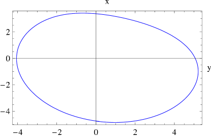
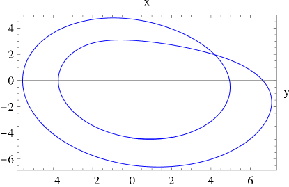
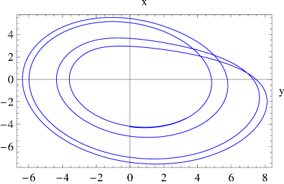
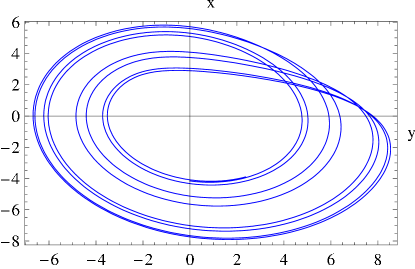
Figure 3: Periodic orbits corresponding to fixed point, period two point, period four point and period eight point for the Poincaré map. Parameter values are $a=2.8$, $a=3.5$, $a=4$ and $a=4.2$.

Before proceeding any further we need to introduce some notation. Let $\Pi=\{(x,y,z)\in\mathbb{R}^{3}\ |\ x=0,x^{\prime}>0\}$ be a Poincaré section. Since for $u\in\Pi$ the first coordinate is equal to zero we will use the remaining two coordinates $u=(y,z)$ to represent a point on $\Pi$. For a fixed parameter value $a>0$ by $P_{a}=(P_{a,y},P_{a,z})\colon\Pi\to\Pi$ we will denote the corresponding Poincaré return map. By $P$ we will denote the map defined by $P(a,y,z)=(a,P_{a,y}(y,z),P_{a,z}(y,z))$.

Apparently the first period doubling bifurcation is observed for $a\approx 2.832445$ and the second one for $a\approx 3.837358$. In the remainder of this section we discuss the computer assisted proof of the existence of both these bifurcations. In our presentation we will discuss the first one more in details, while for the second one we will just state relevant lemmas and estimates.

Let $u_{0}=(y_{0},z_{0})$ be an approximate fixed point for $P_{a_{0}}$, i.e. we set

$$u_{0}=(y_{0},z_{0})=(-4.7946653021070986256,0.052488098609082899093)$$ (38)

and put

$$M=\begin{bmatrix}0.99999765967819775891&-0.9582095926217468751\\ 0.0021634782474835700244&-0.28606708410382636343\end{bmatrix}$$ (39)

The columns of $M$ are normalized approximate eigenvectors of $DP_{a_{0}}(u_{0})$, where first column corresponds to the eigenvalue close to $-1$ and the second one to the eigenvalue close to zero. On section $\Pi$ we choose new coordinates $(\tilde{y},\tilde{z})=M^{-1}((y,z)-u_{0})$ and since, in the sequel, we will use only the new coordinates we will drop the tilde.

Define

$$\begin{array}[]{rcl}A&=&[a_{1},a_{2}]=[2.83244,2.832446]\\ Y&=&[y_{1},y_{2}]=1.3107\cdot[-1,1]\cdot 10^{-3}\\ Z&=&[z_{1},z_{2}]=1.3107\cdot[-1,1]\cdot 10^{-4}\end{array}$$

Now our goal is present the proof of the following theorem

Theorem 10

The map $P_{a}$ has a period doubling bifurcation at some point $(a,y,z)\in{\mathrm{int}}\,(A\times Y\times Z)$.

Remark 11

The existence of period doubling bifurcation is a local phenomenon. In fact the sets $A$, $Y$, $Z$ can be chosen to be smaller which speed up the proof ($13$ minutes versus $87$ minutes), namely we were able to prove the existence of period doubling bifurcation in the set

$$\begin{array}[]{rcl}A&=&[a_{1},a_{2}]=[2.83244,2.832445028]\\ Y&=&[y_{1},y_{2}]=[-1,1]\cdot 10^{-4}\\ Z&=&[z_{1},z_{2}]=[-1,1]\cdot 10^{-5}\end{array}$$

However, the choice of larger set facilitates the proof of the existence of connecting branch of period two points between first and second period doubling bifurcation, because decreasing $a_{2}$ results in the eigenvalue of period-two points to be very close to $1$, which makes it very difficult to rigorously continue it.

6.1 The existence of fixed point curve.

Lemma 12

There exists function $(y_{fp},z_{fp})\colon A\to Y\times Z$ of class $C^{\infty}$ such that for $(a,y,z)\in A\times Y\times Z$ holds

$$P_{a}(y,z)=(y,z)\qquad\text{iff}\qquad(y,z)=(y_{fp}(a),z_{fp}(a))$$

and

$$y_{fp}^{\prime}(A)\subset[-1.3336825610133946629,-1.3275439332565022177]$$ (40)

Proof: The proof, which is computer assisted, consists from two parts, in the first one we prove the existence of the fixed point curve and in the second part we establish estimate (40).

For the first part, we use the Interval Newton Method (Theorem 6) and $C^{1}$-Lohner algorithm to prove that for $a\in A$ there exists a unique fixed point $(y_{fp}(a),z_{fp}(a))$ for $P_{a}$ in $Y\times Z$. In computations we insert the whole set $A\times Y\times Z$ as an initial condition in our routine, which computes the Interval Newton Operator and obtain that the for all $a\in A$ the fixed point $(y_{fp}(a),z_{fp}(a))$ belongs to the set

$$N:=N(\mbox{Id}\,-P_{a},Y\times Z)=\\ \begin{bmatrix}[-2.838378938597049559,3.2727784971172813446]\cdot 10^{-5}\\ [-4.8121450471307824034,4.2979575521536656939]\cdot 10^{-6}\end{bmatrix}^{T}$$ (41)

To obtain (40) we apply $C^{1}$-Lohner algorithm [Z1] to the system

$$\left\{\begin{array}[]{rcl}x^{\prime}&=&-y-z\\ y^{\prime}&=&x+by\\ z^{\prime}&=&b+z(x-a)\\ a^{\prime}&=&0\end{array}\right.$$ (42)

with $b=0.2$ in order to compute a bound for $y_{fp}^{\prime}(A)$. Differentiating

$$P(a,y_{fp}(a),z_{fp}(a))=(a,y_{fp}(a),z_{fp}(a))$$

with respect to $a$ we obtain

$$y_{fp}^{\prime}=\frac{\frac{\partial P_{a,y}}{\partial a}\left(1-\frac{\partial P_{a,z}}{\partial z}\right)+\frac{\partial P_{a,z}}{\partial a}\cdot\frac{\partial P_{a,y}}{\partial z}}{\left(\frac{\partial P_{a,y}}{\partial y}-1\right)\left(\frac{\partial P_{a,z}}{\partial z}-1\right)-\frac{\partial P_{a,y}}{\partial z}\frac{\partial P_{a,z}}{\partial y}}$$ (43)

where the partial derivatives of $P$ are evaluated at $(y_{fp}(a),z_{fp}(a))$.

We use the set $A\times N$, where $N$ is defined in (41) as initial condition in our routine which computes partial derivatives of $P$ and after substituting them to (43) we obtain a bound for $y_{fp}^{\prime}$ as in (40).

We used the Taylor method of order $14$ and the time step equal to $0.02$ to integrate the system (37) in $\mathbb{R}^{3}$ for the first part of the proof and the order $10$ and the time step $0.01$ when we integrate the extended system (42) in the second part.  

Lemma 13

The eigenvalues $\lambda_{1},\lambda_{2}:A\to\mathbb{R}$ of $DP_{a}(y_{fp}(a),z_{fp}(a))$ are given by

$$\lambda_{1}(a) = \frac{1}{2}\left(\frac{\partial P_{a,y}}{\partial y}+\frac{\partial P_{a,z}}{\partial z}-s(a)\right),$$

$$\lambda_{2}(a) = \frac{1}{2}\left(\frac{\partial P_{a,y}}{\partial y}+\frac{\partial P_{a,z}}{\partial z}+s(a)\right),$$

$$s(a) = \sqrt{\left(\frac{\partial P_{a,y}}{\partial y}-\frac{\partial P_{a,z}}{\partial z}\right)^{2}+4\frac{\partial P_{a,y}}{\partial z}\frac{\partial P_{a,z}}{\partial y}}$$

where partial derivatives of $P$ are evaluated at $(y_{fp}(a),z_{fp}(a))$. Let $v(a)$ be the normalized eigenvector corresponding to eigenvalue $\lambda_{1}(a)$. Then

$$\lambda_{1}(a_{1}) \in [-0.99999781944914578613,-0.99999548919217751131]$$

$$\lambda_{1}(a_{2}) \in [-1.00000064581599335217,-1.00000064581598072628]$$

$$\lambda_{2}(A) \subset [-0.0013533261367103342071,0.0013530378340487671934]$$

$$\lambda_{1}^{\prime}(A) \subset [-0.70107900728585614836,-0.62770519734197127715]$$

$$v_{y}(A) \subset \pm[0.99728887963031764841,1.0027184248801992439]$$

where $v_{y}$ denotes the $y$ coordinate of $v$.

Proof: We leave the derivation of formulas for $\lambda_{1},\lambda_{2}$ to the reader. We used the $C^{1}$-Lohner algorithm applied to the system (37) in order to compute bounds for $\lambda_{1}(a_{1})$ and $\lambda_{1}(a_{2})$. Since the parameter $a_{2}$ has been chosen to be very close to the bifurcation parameter we find difficulties with the verification of condition $\lambda_{1}(a_{2})<-1$ in computations performed in interval arithmetics based on double precision (52-bit mantissa) boundary value type. In our computations we used interval arithmetics based on float numbers with $150$-bit mantissa (MPFR [MPFR] and GMP [GMP] packages).

Since the eigenvalue $\lambda_{1}(a)$ of $DP_{a}(y_{fp}(a),z_{fp}(a))$ is given by an explicit formula one can express $\lambda_{1}^{\prime}(a)$ in terms of first and second order partial derivatives of $P$. We obtain

$$\lambda_{1}^{\prime}(a) = \frac{1}{2}\left(\frac{\partial}{\partial a}\frac{\partial P_{a,y}}{\partial y}+\frac{\partial}{\partial a}\frac{\partial P_{a,z}}{\partial z}-s^{\prime}(a)\right)$$

$$s^{\prime}(a) = \frac{1}{s(a)}\left(\frac{\partial P_{a,y}}{\partial y}-\frac{\partial P_{a,z}}{\partial z}\right)\left(\frac{\partial}{\partial a}\frac{\partial P_{a,y}}{\partial y}-\frac{\partial}{\partial a}\frac{\partial P_{a,z}}{\partial z}\right)$$

$$+ \frac{2}{s(a)}\left(\left(\frac{\partial}{\partial a}\frac{\partial P_{a,y}}{\partial z}\right)\frac{\partial P_{a,z}}{\partial y}+\left(\frac{\partial}{\partial a}\frac{\partial P_{a,z}}{\partial y}\right)\frac{\partial P_{a,y}}{\partial z}\right)$$

where the symbols $\frac{\partial}{\partial a}\frac{\partial P_{a,y}}{\partial z}$ and $\frac{\partial}{\partial a}\frac{\partial P_{a,z}}{\partial y}$ should be understood as

$$\frac{\partial}{\partial a}\frac{\partial P_{a,z}}{\partial y}(y_{fp}(a),z_{fp}(a)) = \frac{\partial^{2}P_{a,z}}{\partial a\partial y}(y_{fp}(a),z_{fp}(a))$$

$$+ \frac{\partial^{2}P_{a,z}}{\partial y^{2}}(y_{fp}(a),z_{fp}(a))y_{fp}^{\prime}(a)$$

$$+ \frac{\partial^{2}P_{a,z}}{\partial y\partial z}(y_{fp}(a),z_{fp}(a))z_{fp}^{\prime}(a)$$

and $y_{fp}^{\prime}(a)$ and $z_{fp}^{\prime}(a)$ can be computed as in (43). Next, we applied the $C^{2}$-Lohner algorithm [WZ] to the extended system (42) in order to compute a bound for the first and the second order partial derivatives of $P$ and in consequence a bound for $\lambda_{1}^{\prime}(A)$.

We inserted $A\times N$, where $N$ is defined in (41), as the initial condition in our routine, which computes the partial derivatives of Poincaré map up to second order. In these computations we simultaneously computed bounds for $\lambda_{2}(A)$ and $\lambda_{1}^{\prime}(A)$. The parameter settings of the Taylor method used in the computations are listed in Table 1.

	order	step
$\lambda_{2}(A)$, $\lambda_{1}^{\prime}(A)$	$10$	$0.03$
$\lambda_{1}(a_{1})$	$10$	$0.1$
$\lambda_{1}(a_{2})$ - 150-bit precision	$14$	$0.05$

Table 1: Parameters of the $C^{1}-C^{2}$-Lohner algorithms.

 

6.2 The existence of Liapunov-Schmidt reduction.

Lemma 14

For all $(a,y)\in A\times Y$ there exists unique $z=z(a,y)\in Z$ such that

$$P_{a,z}^{2}(y,z)=z\qquad\text{iff}\qquad z=z(a,y)$$ (44)

and the map $z\colon A\times Y\to Z$ is smooth of class $C^{\infty}$. Moreover, the map $G\colon A\times Y\to\mathbb{R}$ defined by

$$G(a,y)=y-P^{2}_{a,y}(y,z(a,y))$$

satisfies

$$\frac{\partial^{3}G}{\partial y^{3}}(A\times Y)\subset[1.8296823158090675943,7.2204769494502958338]$$ (45)

$$\frac{\partial^{2}G}{\partial y^{2}}(A\times Y)\subset[-0.2084557586786322414,0.2080871792788867581]$$ (46)

Proof: Let us fix $(a,y)\in A\times Y$ and define a function $V_{a,y}\colon Z\to\mathbb{R}$ by $V_{a,y}(z)=z-P_{a,z}^{2}(y,z)$. The computer assisted proof of this Lemma consists of the following steps

• We divide interval $A$ onto $30$ parts. For each subinterval $\bar{A}$ in this covering we proceed as follows

• Using Interval Newton Method (Theorem 6) we verified that for all $(a,y)\in\bar{A}\times Y$ the function $V_{a,y}$ has exactly one zero in $Z$. Denote this zero by $z(a,y)$. This defines the unique map $z\colon\bar{A}\times Y\to Z$ which is smooth by implicit function theorem and which satisfies (44).

• Let $\bar{Z}$ denote a bound for $z(\bar{A},Y)$ resulting from the previous step. Differentiating $z(a,y)-P_{a,z}^{2}(y,z(a,y))=0$ with respect to $y$ we obtain

  $$\left(1-\frac{\partial P_{a,z}}{\partial z}\right)\frac{\partial z}{\partial y} = \frac{\partial P_{a,z}}{\partial y}$$

  $$\left(1-\frac{\partial P_{a,z}}{\partial z}\right)\frac{\partial^{2}z}{\partial y^{2}} = \frac{\partial^{2}P_{a,z}}{\partial z^{2}}(\frac{\partial z}{\partial y})^{2}+2\frac{\partial^{2}P_{a,z}}{\partial y\partial z}\frac{\partial z}{\partial y}+\frac{\partial^{2}P_{a,z}}{\partial y^{2}}$$

  $$\left(1-\frac{\partial P_{a,z}}{\partial z}\right)\frac{\partial^{3}z}{\partial y^{3}} = \frac{\partial^{3}P_{a,z}}{\partial z^{3}}\left(\frac{\partial z}{\partial y}\right)^{3}+3\frac{\partial^{3}P_{a,z}}{\partial y\partial z^{2}}\left(\frac{\partial z}{\partial y}\right)^{2}$$

  $$+ 3\left(\frac{\partial^{2}z}{\partial y^{2}}\frac{\partial^{2}P_{a,z}}{\partial z^{2}}+\frac{\partial^{3}P_{a,z}}{\partial y^{2}\partial z}\right)\frac{\partial z}{\partial y}$$

  $$+ 3\frac{\partial^{2}z}{\partial y^{2}}\frac{\partial^{2}P_{a,z}}{\partial y\partial z}+\frac{\partial^{3}P_{a,z}}{\partial y^{3}}$$

  We see that we can compute all the partial derivatives of $z(a,y)$ as a functions of partial derivatives of $P$. Hence, partial derivatives of $G(a,y)=y-P_{a,y}^{2}(y,z(a,y))$ can be expressed in terms of partial derivatives of $P$.

  Using the $C^{3}$-Lohner algorithm [WZ] applied to the system (37) with a range of parameter values $\bar{A}$ and an initial condition $Y\times\bar{Z}$ we computed bounds of partial derivatives of Poincaré map $P$ up to third order and an estimation for $\frac{\partial^{3}G}{\partial y^{3}}(\bar{A}\times Y)$ and $\frac{\partial^{2}G}{\partial y^{2}}(\bar{A}\times Y)$. The estimates (45) and (46) are an interval enclosures of the estimates obtained in each of $30$ steps.

We used $6$-th order Taylor method with the time step $0.04$, both, to verify the existence of $z(a,y)$ and to compute higher order partial derivatives of $P$.  

6.3 The existence of period doubling bifurcation for $P$.

Lemma 15

For $A=[a_{1},a_{2}]$, $Y=[y_{1},y_{2}]$ the following estimations hold true

$$\frac{\partial G}{\partial y}(a_{2},y_{fp}(a_{2})) \in [-1.2916325,-1.2916323]\cdot 10^{-6}$$ (47)

$$G(a_{2},y_{1}) \in [-1.15,-1.07]\cdot 10^{-13}$$ (48)

$$G(a_{2},y_{2}) \in [5.2,5.21]\cdot 10^{-12}$$ (49)

$$\frac{\partial^{2}G}{\partial y\partial a}(A\times Y) \subset [-2.421398492231531,-0.278863623843693]$$ (50)

$$\frac{\partial G}{\partial y}(\{a_{1}\}\times Y) \subset [0.83,16.87]\cdot 10^{-6}$$ (51)

Proof: The estimations have been obtained using $C^{0}-C^{1}-C^{2}$-Lohner algorithms applied to the systems (37) and (42). The verification of conditions (47–49) required computations in interval arithmetics based on $150$-bit mantissa floating points.

The settings of $C^{0}$-$C^{2}$-Lohner methods for the above computations are listed in Table 2.

	order	step	grid	remarks
$\displaystyle\frac{\partial G}{\partial y}(a_{2},y_{fp}(a_{2}))$	$14$	$0.05$	–	150-bit mantissa
$\displaystyle G(a_{2},y_{1})$	$14$	$0.05$	–	150-bit mantissa
$\displaystyle G(a_{2},y_{2})$	$14$	$0.05$	–	150-bit mantissa
$\displaystyle\frac{\partial^{2}G}{\partial y\partial a}(A\times Y)$	$6$	$0.05$	$5\times 30$	integration of (42)
$\displaystyle\frac{\partial G}{\partial y}(\{a_{1}\}\times Y)$	$10$	$0.05$	$1\times 16000$	nonequal parts

Table 2: Parameters of the $C^{0}-C^{2}$-Lohner algorithms.

 

Proof of Theorem 10: The assertion follows from Theorems 4, 9 and numerical Lemmas 12, 13, 14, 15.

Indeed, assumptions of Theorem 4 has been verified in

• A1 – Lemma 14

• A2 – from Lemma 12 there exists a fixed point curve $(y_{fp},z_{fp})\colon A\to(y_{1},y_{2})$ and from Lemma 14 it has form as desired in A2

• A3 – $0\notin\frac{\partial^{3}G}{\partial y^{3}}(A\times Y)$ because of (45).

  From (46), (50) and (40) it follows that $0\notin\frac{\partial^{2}G}{\partial a\partial y}(A\times Y)+\frac{\partial^{2}G}{\partial y^{2}}y_{fp}^{\prime}(A)\cdot[0,1]$.

  Finally, Lemma 15 guarantees that the remaining assumptions of Lemma 3 with $\varepsilon_{1}=\varepsilon_{\nu}=+1$ and $[\delta_{1},\delta_{2}]=[y_{1},y_{2}]$.

Finally, from Lemma 13 we see that the assumptions about the spectrum of $DP_{a}(A)$ and an eigenvector $v(a)$ as desired in Theorem 9 are satisfied.  

6.4 The existence of second period doubling bifurcation.

In Section 6.3 we gave a computer assisted proof that for some parameter value $\bar{a}_{1}\in[2.83244,2.832446]$ period doubling bifurcation occurs for $P_{\bar{a}_{1}}$. In this section we use similar arguments in order to prove that $P_{\bar{a}_{2}}^{2}$ has period doubling bifurcation for some $\bar{a}_{2}\in[3.83735812,3.837358168411]$.

Since the arguments used to prove the existence of second period doubling bifurcation are the same as in the first period doubling bifurcation we omit the details and we present only the sets and the necessary estimates.

Define

$$A_{2} = [a_{3},a_{4}]=[3.83735812,3.837358168411]$$

$$Y_{2} = [y_{3},y_{4}]=[-1.1,1.1]\cdot 10^{-6}$$

$$Z_{2} = \frac{1}{3}Y_{2}$$

$$u_{2} = (-4.5003284169596655673,0.043136987520848421584)$$

$$M_{2} = \begin{bmatrix}0.99999908059259889903&0.82277742767392003653\\ 0.0013560287448822982113&-0.56836370794614177182\end{bmatrix}$$

The point $u_{2}$ is an approximate period two point for parameter value $a_{4}$, and the columns of matrix $M_{2}$ are normalized eigenvectors of $DP^{2}_{a_{4}}$, where the first column corresponds to eigenvalue close to $-1$.

On the Poincaré section $\Pi$ we will use a coordinates $(y,z)=M^{-1}_{2}(u-u_{2})$, where $u$ denotes a point in cartesian coordinates. In this subsection we will use only these coordinates.

Theorem 16

The Poincaré map $P^{2}_{a}$ has a period doubling bifurcation at some point $(\bar{a}_{2},\bar{y}_{2},\bar{z}_{2})\in{\mathrm{int}}\,(A_{2}\times Y_{2}\times Z_{2})$.

The proof is a consequence of the following lemmas (proved with computer assistance)

Lemma 17

There exist function $(y_{per},z_{per})\colon A_{2}\to Y_{2}\times Z_{2}$ smooth of class $C^{\infty}$ such that for $(a,y,z)\in A_{2}\times Y_{2}\times Z_{2}$ holds

$$P^{2}_{a}(y,z)=(y,z)\qquad\text{iff}\qquad(y,z)=(y_{per}(a),z_{per}(a))$$

and

$$y_{per}^{\prime}(A_{2})\subset[-0.36435039423614490328,-0.36419313389173590956]$$

Lemma 18

Let $\lambda_{1},\lambda_{2}:A\to\mathbb{R}$ be eigenvalues of $DP^{2}_{a}(y_{per}(a),z_{per}(a))$ defined by similar formulas as in Lemma 13. Let $v(a)$ be the normalized eigenvector corresponding to eigenvalue $\lambda_{1}(a)$. Then

$$\lambda_{1}(a_{3}) \in [-0.99999992011934590863,-0.99999992005484927837]$$

$$\lambda_{1}(a_{4}) \in [-1.00000000000149573159618,-1.00000000000149573159615]$$

$$\lambda_{2}(A_{2}) \subset [-7.7304566166653588839,7.7302177026359675856]\cdot 10^{-5}$$

$$\lambda_{1}^{\prime}(A_{2}) \subset [-1.6554066232416912996,-1.6460891324715511974]$$

$$\pi_{y}v(A_{2}) \subset \pm[0.99984657385734598822,1.0001534381577519284].$$

Lemma 19

For all $(a,y)\in A_{2}\times Y_{2}$ there exists unique $z=z(a,y)\in Z_{2}$ such that

$$P_{a,z}^{4}(y,z)=z\qquad\text{iff}\qquad z=z(a,y)$$

and the map $z\colon A_{2}\times Y_{2}\to Z_{2}$ is smooth of class $C^{\infty}$. Moreover, the map $G\colon A_{2}\times Y_{2}\to\mathbb{R}$ defined by

$$G(a,y)=y-P^{4}_{a,y}(y,z(a,y))$$

satisfies

$$\frac{\partial^{3}G}{\partial y^{3}}(A\times Y) \subset [11.780861336872181511,22.544626008881969881]$$

$$\frac{\partial^{2}G}{\partial y^{2}}(A\times Y) \subset [-0.12474597648618415136,0.12474408945310766494]$$

Lemma 20

The following estimations hold true

$$\frac{\partial G}{\partial y}(a_{4},y_{per}(a_{4})) \in [-2.992,-2.991]\cdot 10^{-12}$$

$$G(a_{4},y_{3}) \in [-5.13,-5.11]\cdot 10^{-19}$$

$$G(a_{4},y_{4}) \in [5.21,5.22]\cdot 10^{-19}$$

$$\frac{\partial^{2}G}{\partial y\partial a}(A_{2}\times Y_{2}) \subset [-4.354355790892265432,-2.244876361570084633]$$

$$\frac{\partial G}{\partial y}(\{a_{3}\}\times Y_{2}) \subset [0.99,30.98]\cdot 10^{-8}$$

Parameter settings of computations involved in proofs of the above lemmas are listed in Table 3.

	order	step	grid	remarks
$\displaystyle\frac{\partial^{3}G}{\partial y^{3}}(A_{2}\times Y_{2})$	$10$	$0.04$	$150\times 1$	–
$\displaystyle\frac{\partial^{2}G}{\partial y^{2}}(A_{2}\times Y_{2})$	$10$	$0.04$	$150\times 1$	–
$\displaystyle\frac{\partial G}{\partial y}(a_{4},y_{per}(a_{4}))$	$25$	$0.05$	–	150-bit mantissa
$\displaystyle G(a_{4},y_{3}),G(a_{4},y_{4})$	$25$	$0.05$	–	150-bit mantissa
$\displaystyle\frac{\partial^{2}G}{\partial y\partial a}(A_{2}\times Y_{2})$	$10$	$0.05$	$150\times 1$	integration of (42)
$\displaystyle\frac{\partial G}{\partial y}(\{a_{3}\}\times Y_{2})$	$14$	$0.05$	$1\times 10000$	–

Table 3: Parameters of the $C^{0}-C^{3}$-Lohner algorithms in the proof of the existence of second period doubling bifurcation.

7 Continuation of bifurcation diagram

In the previous sections we proved that the map $P_{a}$ has period doubling bifurcations for parameter values $\bar{a}_{1}\in[a_{1},a_{2}]=A$ and $\bar{a}_{2}\in[a_{3},a_{4}]=A_{2}$ in sets $Y\times Z$ and $Y_{2}\times Z_{2}$, respectively.

Our goal now is to connect these bifurcations with the curve of period two points. More precisely, we prove the following result

Theorem 21

There exists a continuous curve

$$(y_{per},z_{per})\colon(\bar{a}_{1},\bar{a}_{2}]\to\mathbb{R}^{2}$$

of period two points for $P_{a}$. Moreover,

$$(y_{per}(a),z_{per}(a)),P_{a}(y_{per}(a),z_{per}(a)) \in Y\times Z\quad\text{for }\bar{a}_{1}<a\leq a_{2}$$

$$(y_{per}(a),z_{per}(a)),P_{a}^{2}(y_{per}(a),z_{per}(a)) \in Y_{2}\times Z_{2}\quad\text{for }a_{3}\leq a\leq\bar{a}_{2}.$$

Therefore curve $(y_{per},z_{per})$ connects the two bifurcation points for $a=\bar{a}_{1}$ and $a=\bar{a}_{2}$.

The proof of the existence of a branch of period two points for $P$ consists of the following steps.

• the existence of continuous curve of period two points on intervals $(\bar{a}_{1},a_{2}]$ and $[a_{3},\bar{a}_{2}]$ is a consequence of Theorem 10 and Theorem 16, respectively.

• for parameter values slightly above $a_{2}$, $a_{2}<a\leq\tilde{a}$, with $\tilde{a}-a_{2}$ small, we extend this curve using Lemma 8, which requires some $C^{3}$ estimates (hence it is demanding computationally).

• for parameters far from $a_{2}$ up to $a_{3}$, i.e. $\tilde{a}<a\leq a_{3}$, we verify the existence of period two point curves using Krawczyk method (Theorem 7), which requires only $C^{1}$ estimates.

• Since we use different methods for proving the existence of segments of period two points curve over some intervals in $[\bar{a}_{1},\bar{a}_{2}]$ it is necessary to verify that these segments can be glued to produce continuous curve.

At first, it appears that step 2, requiring costly $C^{3}$ computations, is not necessary, because in step 3 we can consider also points close to $a_{2}$ using $C^{1}$ computations. But it turns out that, while in principle possible, this approach may require very large computation times, because the hyperbolicity is very weak there, due to the fact that one eigenvalue of $P^{2}_{a_{2}}$ is very close to $1$.

To deal with this problem we used Lemma 8 to prove that for parameter values slightly above $a_{2}$ there exists a continuous branch of period two points. Algorithm 1 is designed to verify assumptions of Lemma 8. In Lemma 22 we prove its correctness.

Definition 5

Let $U\subset\mathbb{R}^{n}$ be a bounded set. We say that $\mathcal{G}\subset 2^{\mathbb{R}^{n}}$ is a grid of $U$ if

1. $\mathcal{G}$ is a finite set and each $G\in\mathcal{G}$ is a closed set

2. $U\subset\bigcup_{G\in\mathcal{G}}G$

In our algorithms, which will be presented below, we always use grids consisting of interval sets, i.e. sets which are cartesian products of intervals, most of the time uniform grids, which are defined as follows.

Definition 6

Let $Y=\Pi_{i=1}^{n}Y_{i}$, where $Y_{i}=[a_{i},b_{i}]$ for $a_{i}\leq b_{i}$ and let $(g_{1},\dots,g_{n})\in\mathbb{Z}_{+}$. We define a (uniform) $g_{1}\times g_{2}\times\dots\times g_{n}$-grid for $Y$ denoted by $\mathcal{G}(g1_{,}\dots,g_{n},Y)$ as follows.

For any $(j_{1},\dots,j_{n})\in\mathbb{Z}_{+}$, such that $j_{i}\leq g_{i}$ we set

$$g_{j_{1},\dots,j_{n}}=\Pi_{i=1}\left[a_{i},a_{i}+j_{i}\cdot\frac{b_{i}-a_{i}}{g_{i}}\right].$$ (52)

Then $\mathcal{G}(g1_{,}\dots,g_{n},Y)$ is a collection of all $g_{j_{1},\dots,j_{n}}$.

Data: $[\nu_{1},\nu_{2}]$ - an interval, $g_{1},g_{2},g_{3},g_{x}$ - integers, $t\in(0,1)$ - float number, $X\times Y$ - a convex, compact set, $f_{\nu}$ - parameterized family of maps

Result: If algorithms stops and does not throw an exception then assumptions of Lemma 8 are satisfied

begin  $\mathcal{G}_{1}\longleftarrow$ $g_{1}\times g_{x}$-grid for $[\nu_{1},\nu_{2}]\times X$;

foreach $\bar{\nu}\times\bar{X}\in\mathcal{G}_{1}$ do  $y(\bar{\nu},\bar{X})\longleftarrow\mathrm{IntervalNewtonOperator}(\mbox{Id}\,_{Y}-\pi_{Y}\circ f^{2}_{\bar{\nu}}(\bar{X},\cdot),Y,\mathrm{center}(Y))$;

if not $y(\bar{\nu},\bar{X})\subset{\mathrm{int}}\,Y$ then  throw Liapunov-Schmidt reduction not verified   if not $\frac{\partial^{3}G}{\partial x^{3}}(\bar{\nu},\bar{X})>0$ then  throw condition (26) is not satisfied     if (not $G(\nu_{2},\min(X))<0$) or (not $G(\nu_{2},\max(X))>0$) then  throw condition (27) is not satisfied   $\mathcal{G}_{2}\longleftarrow$ $g_{2}$-grid for $[\nu_{1},\nu_{2}]$;

foreach $\bar{\nu}\in\mathcal{G}_{2}$ do  if (not $\frac{\partial G}{\partial\nu}(\bar{\nu},x_{1})>0$) or (not $\frac{\partial G}{\partial\nu}(\bar{\nu},x_{2})<0$) then  throw condition (27) is not satisfied     $\mathcal{G}_{3}\longleftarrow$ $g_{3}$-grid for $[\nu_{1},\nu_{2}]$;

foreach $\bar{\nu}\in\mathcal{G}_{3}$ do  $(\bar{X},\bar{Y})\longleftarrow\mathrm{IntervalNewtonOperator}(\mbox{Id}\,-f_{\bar{\nu}},X\times Y,\mathrm{center}(X\times Y))$;

if not $(\bar{X},\bar{Y})\subset{\mathrm{int}}\,(X\times Y)$ then  throw fixed points curve not verified   $x_{+}\longleftarrow(1-t)\min(X)+t\min(\bar{X})$;

$x_{-}\longleftarrow(1-t)\max(X)+t\max(\bar{X})$;

if (not $G(\min(\bar{\nu}),x_{+})>0$) or (not $G(\min(\bar{\nu}),x_{-})<0$) then  throw condition (28) or (29) is not satisfied   if (not $\frac{\partial G}{\partial\nu}(\bar{\nu},x_{+})<0$) or (not $\frac{\partial G}{\partial\nu}(\bar{\nu},x_{-})>0$) then  throw condition (28) or (29) is not satisfied;

    end

Algorithm 1 verification of assumptions of Lemma 8

Lemma 22

If Algorithm 1 is called with its arguments $\nu_{1},\nu_{2},g_{1},g_{2},g_{3},g_{x},t$, $X\times Y$ and $f_{\nu}$ and it does not throw an exception then the assumptions of Lemma 8 are satisfied for $f_{\nu}$, $\nu\in[\nu_{1},\nu_{2}]$ on $X\times Y$.

Proof: The assumption about existence of fixed point curve is verified in lines 15–19 since for all $\nu\in[\nu_{1},\nu_{2}]$ the Interval Newton Operator satisfies assumptions op Theorem 6.

9

9

9

9

9

9

9

9

9

The existence of Liapunov-Schmidt reduction together with condition (26) is verified in lines 2–8. In lines 4–6 we see that $y(\nu,x)$ which solves equation $y-\pi_{y}(f^{2}_{\nu}(x,y))$ is unique for fixed $\nu$, therefore by the implicit function theorem $y(\nu,x)$ is smooth and we can compute map $G$ and its partial derivatives.

In lines 9–10 we verify that $G(\nu_{2},\min(X))<0$ and $G(\nu_{2},\max(X))>0$. Since $\frac{\partial G}{\partial\nu}(\nu,\min(X))>0$ and $\frac{\partial G}{\partial\nu}(\nu,\max(X))<0$ (lines 11–14) we see that for $\nu\in[\nu_{1},\nu_{2}]$ holds $G(\nu,\min(X))<0$ and $G(\nu,\max(X))>0$. Therefore (27) holds true.

Finally, in lines 15–25 we verify conditions (28–29). Again we verify that for an element of grid $\bar{\nu}$ it holds $G(\min(\bar{\nu}),x_{+})>0$ and $G(\min(\bar{\nu}),x_{-})<0$. This together with $\frac{\partial G}{\partial\nu}(\bar{\nu},x_{+})>0$ and $\frac{\partial G}{\partial\nu}(\bar{\nu},x_{-})<0$ proves (28–29).

 

As was mentioned earlier Algorithm 1 is used to prove the existence of period two points curve for parameter values slightly above the first bifurcation - i.e. for parameters close to $a_{2}$ $G$ has three solutions close to one another. For these parameter values we found difficulties with verifying the existence of period-two points curve using $C^{1}$-computations, only.

For parameter values away from the bifurcation, where all eigenvalues of periodic orbit are well separated from the unit circle, we use Algorithm 2 based on the Newton interval method and the Krawczyk method, both requiring only $C^{1}$-computations, and which verifies the existence of only one branch of period two points for $P_{a}$.

Before we present this algorithm we need to introduce some notations. Let $\bar{\Pi}=\{(x,y,z)\in\mathbb{R}^{3}:x=0\}$ be a Poincaré section for (37) and $\overline{P}_{a}\colon\bar{\Pi}{\mathrel{\longrightarrow\mkern-25.0mu\circ}\;\;}\bar{\Pi}$ be corresponding Poincaré map for a system with parameter value $a$. Notice that the trajectory can intersect $\bar{\Pi}$ at a point $(y,z)\in\bar{\Pi}$ for which $x^{\prime}=-y-z$ is positive or negative (if it is equal to zero the Poincaré map is not defined). Hence we have $\bar{P}^{2}_{a}|_{\Pi}=P_{a}$, where $P_{a}$ is the Poincaré map for section $\Pi=\{(x,y,z)\in\mathbb{R}^{3}\ |\ x=0,x^{\prime}>0\}$ and therefore period two points for $P_{a}$ correspond to period four points for $\bar{P}_{a}$. Let us define a map $F_{a}:\bar{\Pi}^{4}\to\mathbb{R}^{8}$ by

$$F_{a}\begin{bmatrix}(y_{1},z_{1})\\ (y_{2},z_{2})\\ (y_{3},z_{3})\\ (y_{4},z_{4})\end{bmatrix}=\begin{bmatrix}(y_{2},z_{2})-\bar{P}_{a}(y_{1},z_{1})\\ (y_{3},z_{3})-\bar{P}_{a}(y_{2},z_{2})\\ (y_{4},z_{4})-\bar{P}_{a}(y_{3},z_{3})\\ (y_{1},z_{1})-\bar{P}_{a}(y_{4},z_{4})\\ \end{bmatrix}$$

Algorithm 2 was used to verify the existence of a continuous branch of period two points for $P_{a}$ for $a$ belonging to some interval. Sets $X_{i}\times Y_{i}$ give the size of the neighborhood around a candidate periodic orbit on section $\overline{\Pi}$. Lines 4 to 8 constitute a heuristic part and their task is to find a good candidate.

Data: $[a_{*},a^{*}]$ - an interval, $Y_{i}\times Z_{i}$, $i=1,2,3,4$ - convex, compact sets, $g$ - an integer

Result: if algorithm stops and does not throw an exception then there exists a continuous branch of period two points for $P_{a}$ for parameter values $a\in[a_{*},a^{*}]$

begin  $\mathcal{G}\longleftarrow$ $g$-grid for $[a_{*},a^{*}]$;

foreach $\bar{a}\in\mathcal{G}$ do  $a\longleftarrow\mathrm{center}(\bar{a})$;

$u_{1}=(y_{1},z_{1})\longleftarrow$ find approximate period two point for $P^{2}_{a}$ using standard Newton method;

$u_{2}=(y_{2},z_{2})\longleftarrow\bar{P}_{a}(y_{1},z_{1})$;

$u_{3}=(y_{3},z_{3})\longleftarrow\bar{P}_{a}(y_{2},z_{2})$;

$u_{4}=(y_{4},z_{4})\longleftarrow\bar{P}_{a}(y_{3},z_{3})$;

$C\longleftarrow$ compute approximate value of $DF_{a}(u_{1},u_{2},u_{3},u_{4})$;

if $C$ is singular then  $C\longleftarrow\mbox{Id}\,$;

  $U\longleftarrow(u_{1}+Y_{1}\times Z_{1},u_{2}+Y_{2}\times Z_{2},u_{3}+Y_{3}\times Z_{3},u_{4}+Y_{4}\times Z_{4})$;

$u\longleftarrow(u_{1},u_{2},u_{3},u_{4})$;

$K_{\bar{a}}=(k_{1,\bar{a}},k_{2,\bar{a}},k_{3,\bar{a}},k_{4,\bar{a}})\longleftarrow\mathrm{IntervalKrawczykOperator}(F_{\bar{a}},C^{-1},U,u)$;

if not $K_{\bar{a}}\subset{\mathrm{int}}\,U$ then  throw cannot verify the existence of period two point;

  if $k_{1,\bar{a}}\cap k_{3,\bar{a}}\neq\emptyset$ then  throw the unique fixed point for $P^{2}_{\bar{a}}$ in $k_{1,\bar{a}}$ is not necessary period two point for $P_{\bar{a}}$;

    $B\longleftarrow\bigcup_{\bar{a}\in\mathcal{G}}\bar{a}\times k_{1,\bar{a}}$;

if $B$ is not connected then  throw cannot verify if branch of fixed point curve is continuous on interval $[a_{*},a^{*}]$;

  end

Algorithm 2 verification the existence of period two points branch.

16

16

16

16

16

16

16

16

16

16

16

16

16

16

16

16

Lemma 23

If Algorithm 2 is called with its arguments $[a_{*},a^{*}]$, $Y_{i}\times Z_{i}$, $i=1,2,3,4$ and $g$ and does not throw an exception then there exists a continuous curve $(y_{per},z_{per})\colon[a_{*},a^{*}]\to\Pi$ such that $(y_{per}(a),z_{per}(a))$ is period two point for $P_{a}$.

Proof: The existence of fixed point for $P^{2}_{a}$ for all $a\in[a_{*},a^{*}]$ is verified in lines 12–16. Lines 17–18 guarantee that this is a period two point for $P_{a}$, in fact a unique one in $U$.

Uniqueness implies continuity on each $\bar{a}\in\mathcal{G}$ and due to uniqueness and connectedness of the set $B$ defined in line 19 we see that they agree on boundaries of $\bar{a}$.

 

Proof of Theorem 21:

The existence of continuous curve of period two points on intervals $(\bar{a}_{1},a_{2}]$ and $[a_{3},\bar{a}_{2}]$ is a consequence of Theorem 10 and Theorem 16, respectively. Let $a_{s}=2.8329$. For parameter values $[a_{2},a_{s}]$ we verify the existence of period two points branch using Algorithm 1 and for parameter values $a\in[a_{s},a_{3}]$ we use Algorithm 2.

We have ran Algorithm 1 five times with parameters listed in Table 4 (in each case the map is $P_{a}$). Since in each case the algorithm had stopped and did not throw an exception we conclude that in each interval of parameters listed in Table 4 there exist two continuous curves $c_{1}(a)$, and $c_{2}(a)$ of period two points. Sets $X_{i}\times Y_{i}$ listed in Table 4 are chosen so that

$$Y\times Z\subset X_{1}\times Y_{1}\subset\cdots\subset X_{5}\times Y_{5},$$ (53)

where $Y\times Z$ is the set used in the proof of the existence of first period doubling bifurcation. Observe also, that since we know that for $a_{2}$ holds $P_{a_{2}}(c_{1}(a_{2}))=c_{2}(a_{2})$ and $c_{1}(a_{2}),c_{2}(a_{2})\in Y\times Z\subset X_{1}\times Y_{1}$ from Lemma 8 we obtain that $\left\{c_{1}(a),c_{2}(a)\right\}$ is period two orbit for $P_{a}$, for $a\in[a_{2},a_{s}]$, i.e. the whole interval of parameters covered by intervals listed in the first columns in Table 4. The uniqueness of period two orbit together with condition (53) implies that the curves are continuous on $(\bar{a}_{1},a_{s}]$.

One can see that the total number of initial values for which we need compute third order derivatives of $G$,which is equal to the sum of $g_{1}g_{x}$ over all rows in Table 4, is equal to $19350$. The total time of computation of this step is ten hours on the Pentium IV, 3GHz processor.

$[\nu_{1},\nu_{2}]$	$g_{1}$	$g_{2}$	$g_{3}$	$g_{x}$	$t$	$(X_{i}\times Y_{i})\cdot 10^{-4}$
$[a_{2},2.8325]$	$6$	$70$	$600$	$150$	$0.88$	$[-99.0216,97.95]\times[-4,4]$
$[2.8325,2.8326]$	$10$	$80$	$300$	$270$	$0.7$	$[-166.9,163.9]\times[-4,4]$
$[2.8326,2.8327]$	$12$	$60$	$150$	$320$	$0.6$	$[-214.59,209.62]\times[-4,4]$
$[2.8327,2.8328]$	$17$	$50$	$120$	$330$	$0.5$	$[-253.8,246.8]\times[-8,8]$
$[2.8328,2.8329]$	$18$	$50$	$100$	$350$	$0.5$	$[-287.757,279]\times[-8,8]$

Table 4: Parameters of the Algorithm 1.

We have run Algorithm 2 with $74$ different arguments listed in Table 5. We have chosen the parameters of the Algorithm 2 so that such $74$ intervals $[(a_{*})_{i},(a^{*})_{i}]$, $i=1,\ldots,74$ cover the interval $[a_{s},a_{3}]$. Notice also, that for parameters $a$ closer to $a_{s}$ we need larger values of $g$ since the hyperbolicity close to $a_{2}$ is very weak. The total number of subintervals used to cover interval $[a_{s},a_{3}]$ is $614450$. In fact this is the longest part of the numerical proof. The total time of computation of this step is 53 hours on the Pentium IV, 3GHz processor. Since in each case Algorithm 2 stops and does not throw an exception we conclude that on each subinterval $[(a_{*})_{i},(a^{*})_{i}]$ there exists continuous branch of period two points. We need to show that these curves glue continuously at $a^{*}_{i}$’s. In fact, this algorithm returns an upper bound for this period two points branch which is of the form

$$B=\bigcup_{i=1}^{74}B_{i}$$ (54)

where $B_{i}$’s are defined in line 19 of Algorithm 2. We verified that $B$ is connected - this together with an information that for fixed $a\in[a_{s},a_{3}]$ there exists a unique period two point $(y_{per}(a),z_{per}(a))$ such that $(a,y_{per}(a),z_{per}(a))\in B$ implies that the curve $(y_{per}(a),z_{per}(a))$ is continuous on $[a_{s},a_{3}]$.

There remains to show the continuity of fixed point branch for parameter values $a=a_{s}$ and $a=a_{3}$. For $a=a_{s}$ we know that there exist period two points $c_{1}(a_{s}),c_{2}(a_{s})$ which belongs to the last set listed in Table 4, i.e.

$$c_{1}(a_{s}),c_{2}(a_{s})\in W_{1}=u_{0}+M\cdot([-287.757,279]\times[-8,8])\cdot 10^{-4}$$

where $u_{0}$ and $M$ define coordinate system close to first period doubling bifurcation and are defined in (38–39). On the other hand the estimation for period two point resulting from Krawczyk method used in Algorithm 2 is

$$W_{2} = (W_{2}^{1},W_{2}^{2})$$

$$W_{2}^{1} = [-4.7668051788293892557,-4.7667832743925968586]$$

$$W_{2}^{2} = [0.052543190547910088861,0.052543238016254205369]$$

One can verify that $W_{2}\subset W_{1}$ which obviously means that a period two point $(y_{per}(a_{s}),z_{per}(a_{s}))\in W_{2}$ resulting from the Krawczyk method and Algorithm 2 is one of the points $c_{1}(a_{s}),c_{2}(a_{s})$ resulting from Algorithm 1. Hence, the curve of period two points is continuous at $a=a_{s}$.

In a similar way we verified continuity at $a=a_{3}$. From the Krawczyk method used in Algorithm 2 we know that $(y_{per}(a_{3}),z_{per}(a_{3}))$ is a unique period two point in the set

$$W_{3} = (W_{3}^{1},W_{3}^{2})$$

$$W_{3}^{1} = [-4.5010116820607413146,-4.4996232549240025023]$$

$$W_{3}^{2} = [0.043134233933640332703,0.043140290681655812932]$$

On the other hand from Theorem 16 we know that for $a=a_{3}$ period two point belongs to the set

$$W_{4}=u_{2}+M_{2}\cdot(Y_{2}\times Z_{2})$$

where $M_{2}$, $u_{2}$, $Y_{2},Z_{2}$ define the set on which we verify the existence of second period doubling bifurcation. One can verify that $W_{4}\subset W_{3}$ which proves that the branch of period two points is continuous at $a=a_{3}$.

 

$U=[-1,1]\cdot(1100,3,1000,3000,1100,3,1000,3000)\cdot 10^{-8}$
$i$	$[a_{*},a^{*}]$	$g$	$Y_{1}\times Z_{1}\times Y_{2}\times Z_{2}\times Y_{3}\times Z_{3}\times Y_{4}\times Z_{4}$
$1$	$[2.8329,2.83291]$	$14000$	$U$
$2$	$[2.83291,2.83292]$	$13500$	$U$
$3$	$[2.83292,2.83293]$	$12200$	$3U$
$4$	$[2.83293,2.83294]$	$11250$	$3U$
$5$	$[2.83294,2.83295]$	$10400$	$3U$
$6$	$[2.83295,2.83296]$	$9650$	$3U$
$7$	$[2.83296,2.83297]$	$9050$	$3U$
$8$	$[2.83297,2.83298]$	$8500$	$3U$
$9$	$[2.83298,2.83299]$	$8000$	$3U$
$10$	$[2.83299,2.833]$	$7550$	$3U$
$11$	$[2.833,2.83301]$	$7200$	$3U$
$12$	$[2.83301,2.83302]$	$6800$	$3U$
$13$	$[2.83302,2.83303]$	$6500$	$3U$
$14$	$[2.83303,2.83304]$	$6200$	$3U$
$15$	$[2.83304,2.83305]$	$6000$	$3U$
$16$	$[2.83305,2.83306]$	$5700$	$3U$
$17$	$[2.83306,2.83307]$	$5500$	$3U$
$18$	$[2.83307,2.83308]$	$5300$	$3U$
$19$	$[2.83308,2.83309]$	$5100$	$3U$
$20$	$[2.83309,2.8331]$	$4900$	$3U$
$21$	$[2.8331,2.83311]$	$4800$	$3U$
$22$	$[2.83311,2.83312]$	$4600$	$3U$
$23$	$[2.83312,2.83313]$	$4450$	$3U$
$24$	$[2.83313,2.83314]$	$4300$	$3U$
$25$	$[2.83314,2.83315]$	$4150$	$3U$
$26$	$[2.83315,2.83316]$	$4050$	$3U$
$27$	$[2.83316,2.83317]$	$3950$	$3U$
$28$	$[2.83317,2.83318]$	$3850$	$3U$
$29$	$[2.83318,2.83319]$	$3750$	$3U$
$30$	$[2.83319,2.8332]$	$3650$	$3U$
$31$	$[2.8332,2.8333]$	$36000$	$3U$
$32$	$[2.8333,2.8334]$	$29000$	$3U$
$33$	$[2.8334,2.8335]$	$24000$	$3U$
$34$	$[2.8335,2.8336]$	$20000$	$3U$
$35$	$[2.8336,2.8337]$	$18000$	$3U$
$36$	$[2.8337,2.8338]$	$16000$	$3U$
$37$	$[2.8338,2.8339]$	$14000$	$3U$
$38$	$[2.8339,2.834]$	$13000$	$3U$
$39$	$[2.834,2.8345]$	$59000$	$3U$
$40$	$[2.8345,2.835]$	$42000$	$3U$
$41$	$[2.835,2.8355]$	$17500$	$15U$
$42$	$[2.8355,2.836]$	$11000$	$15U$
$43$	$[2.836,2.8365]$	$8000$	$15U$
$44$	$[2.8365,2.837]$	$6200$	$15U$
$45$	$[2.837,2.8372]$	$2800$	$30U$
$46$	$[2.8372,2.8375]$	$3600$	$30U$
$47$	$[2.8375,2.838]$	$5000$	$30U$
$48$	$[2.838,2.8385]$	$3600$	$30U$
$49$	$[2.8385,2.839]$	$2900$	$30U$
$50$	$[2.839,2.8395]$	$2400$	$30U$
$51$	$[2.8395,2.84]$	$2100$	$30U$
$52$	$[2.84,2.841]$	$3700$	$30U$
$53$	$[2.841,2.842]$	$3000$	$30U$
$54$	$[2.842,2.843]$	$2500$	$30U$
$55$	$[2.843,2.844]$	$2200$	$30U$
$56$	$[2.844,2.845]$	$2000$	$30U$
$57$	$[2.845,2.846]$	$1700$	$30U$
$58$	$[2.846,2.848]$	$3100$	$30U$
$59$	$[2.848,2.85]$	$2600$	$30U$
$60$	$[2.85,2.86]$	$11000$	$30U$
$61$	$[2.86,2.87]$	$6500$	$30U$
$62$	$[2.87,2.88]$	$4700$	$30U$
$63$	$[2.88,2.89]$	$3700$	$30U$
$64$	$[2.89,2.9]$	$3100$	$30U$
$65$	$[2.9,2.95]$	$4400$	$150U$
$66$	$[2.95,3]$	$2500$	$150U$
$67$	$[3,3.1]$	$3500$	$150U$
$68$	$[3.1,3.2]$	$2500$	$150U$
$69$	$[3.2,3.3]$	$2100$	$150U$
$70$	$[3.3,3.4]$	$1800$	$150U$
$71$	$[3.4,3.5]$	$1600$	$150U$
$72$	$[3.5,3.6]$	$1400$	$150U$
$73$	$[3.6,3.7]$	$1500$	$150U$
$74$	$[3.7,a_{3}]$	$2400$	$150U$

Table 5: Parameters of Algorithm 2. The initial set $U$ is defined in the first line of the table.

7.1 Technical data.

In order to compute Poincaré maps $P$ and $P^{2}$ with their partial derivatives we used the interval arithmetic [IE, Mo], the set algebra and the $C^{r}$-Lohner algorithm [WZ] developed at the Jagiellonian University by the CAPD group [CAPD]. The C++ source files of the program with an instruction how it should be compiled and run are available at [WI].

All computations were performed with the Pentium IV, 3GHz processor and 512MB RAM under Kubuntu Feisty Fawn linux with gcc-4.1.1 and MS Windows XP Professional with gcc-3.4.4. The computations took approximately three days. The main time-consuming part (over 63 hours) is the verification of the existence of connecting branch of period two points between first and second bifurcation.

References

• [A] G. Alefeld, Inclusion methods for systems of nonlinear equations - the interval Newton method and modifications, in Topics in Validated Computations, J. Herzberger (Editor), Elsevier Science B.V., 1994, pages 7–26
• [An] A. Andronov, Mathematical Problems of self-oscillation theory, in I All-Union Conference on Oscillations, November 1931, GTTI, Moscow-Leningrad 1933, pp. 32–71
• [AK] G. Arioli, H. Koch, Computer-assisted methods for the study of stationary solutions in dissipative systems, applied to the Kuramoto-Sivashinski equation, preprint 2005
• [AAIS] V. Arnold, V. Afraimovich, Y. Ilyashenko, L. Silnikov, Theory of Bifurcations, in V. Arnold ed., Dynamical Systems, 5. Encyclopaedia of Mathemical Sciences, 1994, Springer-Verlag New York
• [BC] M. Benedicks, L. Carleson, The dynamics of the H non map. Ann. of Math. (2) 133 (1991), no. 1, 73–169.
• [CAPD] CAPD – Computer Assisted Proofs in Dynamics group, a C++ package for rigorous numerics, http://capd.wsb-nlu.edu.pl.
• [CH] S.-N. Chow and J. Hale, Methods of Bifurcation Theory, Springer–Verlag, New York, 1982
• [G] G. Iooss, Bifurcation of Maps and Applications, North-Holland, 1979
• [GMP] GNU Multiple Precision Arithmetic Library, http://gmplib.org
• [H] J. Hale, Stability from the bifurcation function, Differential equations (Proc. Eighth Fall Conf., Oklahoma State Univ., Stillwater, Okla., 1979), Ed. Ahmed, Keener, Lazer, pp. 23–30, Academic Press, New York-London-Toronto, Ont., 1980.
• [HK] S.-N. J. Hale and H. Kocak, Dynamics and Bifurcations, Springer–Verlag, New York, 1986
• [HPS] M.W. Hirsch, C.C. Pugh and M. Shub, Invariant manifolds, Lecture Notes in Mathematics vol. 583, 1997
• [IE] The IEEE Standard for Binary Floating-Point Arithmetics, ANSI-IEEE Std 754, (1985).
• [K] A. Kelley, The Stable, Center-Stable, Center-Unstable, Unstable Manifolds. An Appendix in Transversal Mappings and Flows by R. Abraham and J. Robbin, Benjamin, New York, 1967
• [Kr] R. Krawczyk, Newton-Algorithmen zur Bestimmung von Nullstellen mit Fehlerschanken, Computing 4, 187 -201 (1969).
• [Ku] Y. Kuzniecov, Elements of Applied Bifurcation Theory, Applied Mathematical Sciences vol. 112, Springer 1994
• [Lo] R.J. Lohner, Computation of Guaranteed Enclosures for the Solutions of Ordinary Initial and Boundary Value Problems, in: Computational Ordinary Differential Equations, J.R. Cash, I. Gladwell Eds., Clarendon Press, Oxford, 1992.
• [MM] K. Mischaikow, M. Mrozek, The Conley Index Theory, in: Handbook of Dynamical Systems III: Towards Applications, Editors: B. Fiedler, G. Iooss, N. Kopell, Elsevier Science B. V., Singapore 2002, 393-460.
• [MPFR] A C library for multiple-precision floating-point computations with correct rounding, http://www.mpfr.org.
• [Mo] R.E. Moore, Interval Analysis. Prentice Hall, Englewood Cliffs, N.J., 1966
• [MV] L. Mora, M. Viana, Abundance of strange attractors. Acta Math. 171 (1993), no. 1, 1–71.
• [N] A. Neumeier, Interval methods for systems of equations, Cambridge University Press, 1990.
• [NJ] N.S. Nedialkov , K.R. Jackson, An interval Hermite-Obreschkoff method for computing rigorous bounds on the solution of an initial value problem for an ordinary differential equation. in Developments in reliable computing (Budapest, 1998), 289–310, Kluwer Acad. Publ., Dordrecht, 1999.
• [OH] J.C. F. de Oliveira and J. Hale, Dynamic behavior from bifurcation equations, T hoku Math. J. (2) 32 (1980), no. 4, 577–592.
• [P] P. Pilarczyk, Topological numerical approach to the existence of periodic trajectories in ODE’s, Discrete and Continuous Dynamical Systems, A Supplement Volume: Dynamical Systems and Differential Equations, 701-708 (2003)
• [R] O.E. Rössler, An Equation for Continuous Chaos, Physics Letters Vol. 57A no 5, pp 397–398, 1976.
• [T] R. Thom, Stabilité Structurelle et Morphogenése, Benjamin New York 1972
• [WI] D. Wilczak, http://www.ii.uj.edu.pl/~wilczak, a reference for auxiliary materials.
• [WY1] Q. Wang, L.-S. Young, Strange attractors with one direction of instability. Comm. Math. Phys. 218 (2001), no. 1, 1–97
• [WY2] Q. Wang, L.-S. Young, From invariant curves to strange attractors. Comm. Math. Phys. 225 (2002), no. 2, 275–304
• [WZ] D. Wilczak, P. Zgliczyński, $C^{r}$-Lohner algorithm, submitted, available at http://www.ii.uj.edu.pl/~wilczak.
• [Z1] P. Zgliczyński, $C^{1}$-Lohner algorithm, Foundations of Computational Mathematics, 2 (2002), 429–465.
• [Z2] P. Zgliczyński, Towards an rigorous steady states bifurcation diagram for the Kuramoto-Sivashinsky equation - a computer assisted rigorous approach, http://www.ii.uj.edu.pl/~zgliczyn
• [Z3] P. Zgliczyński, Computer assisted proof of chaos in the Hénon map and in the Rössler equations, Nonlinearity, 1997, Vol. 10, No. 1, 243–252.