Measurement of the charged kaon lifetime with the KLOE detector

Abstract:

We have measured the charged kaon lifetime using a sample of 15 $\times$ 10⁶ tagged kaon decays. Charged kaons were produced in pairs at the DA$\Phi$NE $\phi$-factory, $e^{+}e^{-}\to\phi\to K^{+}K^{-}$. The decay of a $K^{+}$ was tagged by the production of a $K^{-}$ and viceversa. The lifetime was obtained, for both charges, from independent measurements of the decay time and decay length distributions. From fits to the four distributions we find $\tau$ = (12.347$\pm$0.030) ns.

1 Introduction

While the lifetime of the $K_{S}$ is well measured and measurements of the lifetime of the $K_{L}$ [1],[2] have been recently performed, the most precise measurement of the lifetime of the charged kaon dates back to 1971: $\tau_{\pm}=(12.380\pm 0.016)$ ns [3]. At the time, the agreement with previous measurements was poor and more recent measurements did not improve the agreement. The 2006 PDG [4] gives $\tau_{\pm}=(12.385\pm 0.025)$ ns corresponding to an accuracy of 0.2$\%$. However the set of measurements upon which the above value is based is not self consistent. The probability that the spread of the values used by PDG be due to the statistical fluctuations is very low, 0.17$\%$. Averaging an inconsistent set is not a valid procedure. The PDG in fact enlarges the errors by a factor of 2.1. It is important therefore to confirm the value of $\tau_{\pm}$. We report in the following on new measurements of $\tau_{\pm}$. The statistical error on the lifetime obtained fitting a decay curve over a time interval $\Delta$t is given by:

$$\frac{\delta\tau}{\tau}=\frac{1}{\sqrt{N}}\times\frac{e^{T}-1}{\sqrt{1+e^{2T}-e^{T}(2+T^{2})}}$$ (1)

where T = $\Delta$t/$\tau$ is the time interval in $K^{\pm}$-lifetime units. With $T\approx 2$ and number of events $N\approx 4\times 10^{6}$, the best statistical accuracy reachable in our case is $0.1\%$, if no other sources of statistical error were present. We have developed two different methods, one employing the reconstruction of the kaon path length and the other measuring directly the kaon decay time.

2 The KLOE detector

Data were collected with the KLOE detector at DA$\Phi$NE [5], the Frascati $e^{+}e^{-}$ collider operated at a center of mass energy $W=M_{\phi}\sim$1020 MeV. Equal-energy positron and electron beams collide with a crossing angle of $\pi-25$ mrad, which results in a small transverse momentum ( $p_{\phi}\sim$ 12.5 MeV) of the $\phi$ mesons produced. The beam spot has $\sigma_{x}\approx$ 2 mm $\sigma_{y}\approx$ 0.02 mm and $\sigma_{z}\approx$ 30 mm. The KLOE detector is inserted in a 0.52 T magnetic field. It consists of a large cylindrical drift chamber (DC), surrounded by a fine sampling lead-scintillating fibers calorimeter (EMC). The DC [6], 4 m diameter and 3.3 m long, has full stereo geometry and operates with a gas mixture of 90% Helium and 10% Isobutane. Momentum resolution for tracks with large PT is $\sigma(p_{\bot})/p_{T}\sim 0.4\%$. Spatial resolution is $\sigma_{r\phi}\sim 150\mu$m and $\sigma_{z}\sim$ 2 mm. Vertices are reconstructed with a 3D accuracy of $\sim$3 mm. The DC inner walls are made in carbonium fibers with thickness of $\sim$1 mm. The beam pipe walls are made of AlBeMet, an alloy of beryl-aluminum 60$\%$-40$\%$, with thickness of $\sim$0.5 mm. The EMC [7], divided into a barrel and two endcaps, for a total of 88 modules, covers 98% of the solid angle. Arrival times of particles, 3D positions and the energy deposits are obtained from readout of signals on both ends of the module, with a granularity of $\sim$ 4.4 $\times$ 4.4 cm², for a total of 2240 cells arranged in five layers. Cells close in time and space are grouped into a calorimeter cluster. Resolution on energy and time measurement are $\sigma_{E}/E=5.7\%/\sqrt{E(\rm{GeV})}$ and $\sigma_{T}=57\textrm{ps}/\sqrt{E(\rm{GeV})}\oplus 100\;\textrm{ps}$. The trigger [8], used for this analysis, is based on the coincidence of at least two local energy deposits in the EMC, above a threshold of 50 MeV in the barrel and 150 MeV in the end caps. Cosmic rays muons crossing the detector are vetoed. Since the trigger time formation is larger than the interbunch time ($\sim$ 2.7 ns), the trigger operates in continuous mode and its signal is synchronized with the DA$\Phi$NE accelerator Radio Frequency. The trigger $T_{0}$ for an event is thus displaced in time with respect to the correct crossing by an integer multiple of the interbunch time which is different event by event. The correct bunch crossing is found after the event reconstruction. For this analysis a sample 3$\times 10^{8}$of $\phi\to K^{+}K^{-}$, events generated with the KLOE MonteCarlo (MC)[9], has been used.

3 The tag procedure

$\phi$-mesons decay, in their rest frame, into anti-collinear $K\bar{K}$ pairs. In the laboratory this remains approximately true because of the small $\phi$-meson $\beta$. The detection of a $K^{+}(K^{-})$ tags the presence of a $K^{-}(K^{+})$ of given momentum and direction. The decay products of the $K^{+}K^{-}$ pair define two spatially separated regions called the tag and the signal hemispheres. Identified $K^{\mp}$ decays tag a $K^{\pm}$ sample of known total count $\mathcal{N}$. This procedure is a unique feature of a $\phi$-factory and allows to measure absolute branching ratios. For this analysis charged kaons are tagged using the $K^{\pm}\rightarrow\mu^{\pm}\hbox to0.0pt{\raise 5.16663pt\hbox{\scriptsize($-$)}\hss}\kern 3.00003pt\nu_{\,\mu}$ ($K_{\mu 2}$) decay. This decay corresponds to about 63% of the charged kaon decay width [4] and since $BR(\phi\rightarrow K^{+}K^{-})\simeq 49\%$ [4] and $\sigma(e^{+}e^{-}\to\phi)\sim$ 3 $\mu$b, there are about $1.1\times 10^{6}K^{+}K^{-}$ events/pb^-1. The $K_{\mu 2}$ decay is clearly identified since it exhibits a peak, reconstucted with a resolution of about 1 MeV, at $\approx$ 236 MeV in the momentum spectrum of the secondary tracks in the kaon rest frame. In order to minimize biases to trigger efficiency, we ensure that the tagging kaon did provide the trigger of the event by requiring a cluster in the EMC (associated to the muon track) which satisfies the trigger conditions. Hereafter these events are called self-triggered tags. We find $N_{\rm selftrg\ tag}\approx 1.2\times 10^{5}$ per pb^-1. The MC simulation shows that the contamination of the selected $\phi\rightarrow K^{+}K^{-}$ sample is negligible. The $K_{\mu 2}$ tag allows a precise determination of the correct bunch crossing of the event using the muon and kaon track lengths and the momenta measured in the DC and the arrival time of the muon in the EMC. The tagging efficiency is almost independent on the proper decay time of the signal kaon. The small residual correlation has been evaluated with the Monte Carlo and checked with data using doubly tagged events, the events in which both the $K^{+}$ and the $K^{-}$ are reconstructed and tag the event.

4 Signal selection

The measurement is performed using data from an integrated luminosity $\mathcal{L}$= 210 pb^-1 collected at the $\phi$ peak. The average $\phi-$meson momentum and the coordinates of the $e^{+}e^{-}$ interaction point (IP) are measured run by run with Bhabha scattering events. $K_{\mu 2}$ tags of both charges have been used. We developed two analysis methods: the kaon decay length and the kaon decay time. The two methods have comparable precision and different systematics; this allows a useful cross-check of the results. We use a coordinate system where the x-axis points to the center of the collider, the z-axis bisects the two beam lines and the y-axis is vertical. For both methods the kaon decay vertex position $(x,y,z)$ is searched for in a fiducial volume (FV) defined by:

$$40\ \mbox{cm}<R<150\ \mbox{cm},\kern 14.22636pt|z|\leq 150\ \mbox{cm}$$ (2)

where $R=\sqrt{x^{2}+y^{2}}$.

4.1 Kaon decay length method

The measurement of the charged kaon decay length requires the reconstruction of the kaon decay vertex using only DC-information. We use any kaon decay mode. The evaluation of the vertex reconstruction efficiency uses a data control sample obtained by EMC-information only. Given a charged kaon fulfilling the self-triggering tag requirements, our signal is given by the opposite charged kaon decaying in the FV. The signal kaon track reconstructed in the DC must satisfy the following requests:

$$R_{\rm{PCA}}<10\ \mbox{cm},$$

$$|z_{\rm{PCA}}|<20\ \mbox{cm},$$ (3)

$$70<p_{K}<130\ \mbox{MeV}.$$

where $R_{\rm{PCA}}=\sqrt{x^{2}_{\rm{PCA}}+y^{2}_{\rm{PCA}}}$ and PCA indicates the point of closest approach of the kaon track to the interaction point. The low level of background allows to keep these cuts very loose, even accounting for the effect of multiple scattering and energy loss of the kaon in the DC wall and into the beam pipe. We ask the reconstruction of a vertex formed by the kaon track and one of its charged decays, lying inside the FV. The only source of background is given by events in which one kaon track is split in two pieces by the reconstruction algorithm so as to mimic a decay vertex. This happens for kaon with low $p_{t}$ which describe cirles in the DC. In order to reject these events we used the momentum of the charged secondary particle ($p^{\ast}$) evaluated in the kaon rest frame, using the kaon mass hypothesis. With the cut $p^{\ast}>100$ MeV we lose about 5.4% of signal and we reduce this background to the 0.46% level. Since charged kaons have an average velocity $\beta\approx$ 0.2 they lose a non negligible fraction of their energy traversing the beam pipe and DC walls and in the DC gas. Therefore, given the decay length, we have to correct for the corresponding change in $\beta$, of the order of 25$\%$, to evaluate the proper time. Once the decay vertex has been identified, the kaon track is extrapolated backwards to the interaction point in 5 mm steps, $\Delta l_{i}$, taking into account the average ionization energy loss $dE/dx$ to evaluate its velocity $\beta_{i}$ in each step. The kaon proper decay time, $t^{*}$ is finally evaluated as

$$t^{*}=\sum_{i}\Delta t_{i}=\sum_{i}\frac{\sqrt{1-\beta^{2}_{i}}}{\beta_{i}}\frac{\Delta l_{i}}{c}$$ (4)

In the range $12<t^{*}<40$ ns we collected $1.7\times 10^{6}$ events. The average resolution in $t^{*}$, evaluated from MC simulation, is of the order of 1 ns, see fig. 1 and its effects are taken into account in the fit procedure by means of a resolution smearing matrix, as described in section 6, which makes the resolution folding.

4.2 Kaon decay time method

The second method relies on the measurement of the kaon decay time using EMC information only for the signal side. We consider events with a $\pi^{0}$ in the final state:

$$K^{\pm}\rightarrow X+\pi^{0}\rightarrow X+\gamma\gamma$$ (5)

In this case the reconstruction efficiency of the kaon decay vertex is evaluated using a data control sample given by DC information only. We obtain the kaon decay time using the photon arrival time to the EMC. From the measured momenta of the $\phi$-meson and of the tagging kaon we can evaluate the momentum of the signal kaon at the IP and build the expected path of the signal kaon: it is obtained by geometrical step by step extrapolation, corrected for local magnetic field and energy loss effects. Then we look for clusters not associated to tracks in the DC, “neutral” clusters. Among these we select as photon candidates the two (or three, if present) most energetic clusters with:

$$24^{\circ}<\theta_{\rm{cl}}<156^{\circ}$$

$$T_{0}<t_{\rm{cl}}<T_{0}+70~{}\rm{ns}$$ (6)

where $\theta_{cl}$ is the polar angle, the angle between the position of the cluster with respect the IP and the z axis, $t_{cl}$ is the time of the cluster, and $T_{0}$ is the $\phi$ decay time evaluated considering the $K_{\mu 2}$ decay chain on the tagging side. These cuts are used to reject the machine background. The request of three neutral clusters allows us to select also the events with the track of the charged decay particle not associated to its calorimeter cluster.
Then we move along the expected path of the signal kaon in 5 mm steps and at each step we look for the $\pi^{0}\to\gamma\gamma$ decay vertex by minimizing a $\chi^{2}$ function:

$$\chi^{2}=\frac{(M_{\gamma\gamma}-M_{\pi^{0}})^{2}}{\sigma_{M_{\pi^{0}}}^{2}}+\frac{\Delta t_{12}^{2}}{\sigma_{t_{12}}^{2}}+\frac{(t_{K}-t_{cl})^{2}}{\sigma_{t}^{2}}$$ (7)

In Eq. (7) $M_{\gamma\gamma}$ is the invariant mass of the two photon candidates, $M_{\pi^{0}}$ is the $\pi^{0}$ mass and $\sigma_{M_{\pi^{0}}}\simeq 17$ MeV is the resolution on the $\pi^{0}$ mass; $\Delta t_{12}$ is defined as:

$$\Delta t_{12}=(t_{\gamma_{1}}-r_{1}/c)-(t_{\gamma_{2}}-r_{2}/c)$$ (8)

where $t_{\rm{\gamma_{i}}}$ is the time of the i-th neutral cluster, $r_{i}$ is the distance of the neutral cluster from the candidate kaon decay vertex; $\sigma_{t_{12}}$ is obtained by propagating the errors on the equation 8. $t_{K}$ is the time of flight of the charged kaon measured along the kaon path, $t_{cl}$ is the time of flight of the charged kaon given by the weighted mean of the arrival time of the two photons; $\sigma_{t}$ is the uncertainty on the kaon decay time obtained from the selected neutral clusters, of the order of few hundreds ps. In case three clusters have been selected we choose the pair with best $\chi^{2}$. The position along the signal kaon path that gives the minimum value of the $\chi^{2}$ defines the $K^{\pm}\rightarrow X+\pi^{0}\rightarrow X+\gamma\gamma$ decay point and is accepted if lying inside the FV. Moreover we require:

$$\chi^{2}<30,$$

$$80~{}\rm{MeV}<M_{\gamma\gamma}<200~{}\rm{MeV},$$ (9)

$$\left|\frac{\Delta t_{12}}{\sigma_{t_{12}}}\right|<5.$$

The charged kaon proper time is obtained from:

$$t^{*}=\frac{t_{cl}}{\langle\gamma\rangle}$$ (10)

Where $\langle\gamma\rangle$ is the average between the charged kaon Lorentz factor $\gamma$ at the IP and at the decay vertex. This approximation is appropriate because the variation of $\gamma$ along the decay path is of the order of 1$\%$. The average $t^{*}$ resolution of the events selected is better than 1 ns, see fig. 1. The secondary peaks at $\pm$n$\times$2.7 ns are due to events with an incorrect bunch crossing determination. In the range between 10 and 50 ns we collected $8\times 10^{5}$ events.

Figure 1: $t^{*}$ resolution from kaon path length measurement (left) and from kaon decay time measurement (right). The side lobes at $\pm$n$\times$2.7 ns in the right plot are events with incorrect bunch crossing time determination. This effect is absent for the length measurement.

5 Efficiency evaluation

In order to be as little dependent as possible from the MonteCarlo simulation and from possible differences between data and MonteCarlo, we measured directly on data the reconstruction efficiency of the kaon decay vertex, as a function of the charged kaon proper time, for both methods. A data control sample for the efficiency of the first method, using DC information for signal selection, is obtained from the signal selection of the second method, based on EMC information only, and viceversa. What is relevant for the fit is the efficiency behavior as a function of $t^{*}$ rather than its absolute value. In both cases the efficiency has been obtained in bins of $t^{*}$ using the definitions (10) and (4) respectively. We applied the same method on MonteCarlo events and we compared the efficiencies obtained with this method (MC datalike efficiencies) with the MC true efficiencies, determined as functions of the true proper time including all the decay modes used for each method ($K^{\pm}\to all$ for the first method and $K^{\pm}\to X\pi^{0}$ for the second method). Fig. 2 shows a comparison between the MC true and the MC datalike efficiencies. For the first method it is important to stress that even if the control sample is obtained reconstructing kaon decays with a $\pi^{0}$ in the final state, datalike efficiency reproduces the true one obtained reconstructing all the kaon decay modes. Fig. 3 shows the ratio of the efficiency measured on data over the MC datalike efficiency, for both methods. For the kaon decay length method, the efficiency measured on data in the range [5, 20] ns is different in shape from the MC efficiency. The highly ionizing charged kaon fires multiple hits in the small cells of the DC, i.e. in the inner 12 layers of detector. This effect has been introduced in the MC simulation afterwards. For this reason we used the efficiency evaluated directly data with the small, $\mathcal{O}$(10^-4), correction given by the ratio of the MC true efficiencies over MC datalike efficiencies.

Figure 2: Left: charged vertex reconstruction efficiency as function of the charged kaon proper time. Right: $\pi^{0}$ decay vertex efficiency as a function of the charged kaon proper time. Dots (open circles) represent MC datalike (MC true) efficiencies.

Figure 3: Left: ratio between the charged vertex reconstruction efficiency as function of the charged kaon proper time evaluated on data and the MC datalike one. Right: ratio between the $\pi^{0}$ decay vertex efficiency as a function of the charged kaon proper time evaluated on data and the MC datalike one.

6 Fit to the proper time distribution

The fit to the proper time distribution is done comparing the observed with the expected distribution and minimizing a $\chi^{2}$ function. The entries in each bin of the expected histogram are given by the integral of the exponential decay function (which depends only on the kaon lifetime) corrected for the efficiency curve; a smearing matrix accounts for the effect of the resolution. We fit the proper time distribution in the time interval where we have good agreement between MC true and MC datalike efficiencies. The efficiency profiles obtained on data as in section 5 are corrected for the tiny residual difference between the MC true and MC datalike shapes, and for the small effect of the tag-signal hemispheres correlation; the overall corrections is of $\mathcal{O}$(10^-3) for both methods. The resolution function is evaluated in slices of the order of few nanoseconds on a MC data sample of about 175 pb^-1 of $\phi\rightarrow K^{+}K^{-}$ events. We then define the $N\times N$ smearing matrix, whose element $s_{ji}$ gives the fraction of events generated in the i-th bin but reconstructed in the $j-th$ bin. We chose a bin size of 1 ns in order to reduce the statistical fluctuations and the relative importance of the smearing corrections. We then minimize

$$\chi^{2}=\sum_{j=1}^{N_{\rm{fit}}}\frac{(N^{\rm{obs}}_{j}-N^{\rm{ex}}_{j})^{2}}{(\sigma^{\rm{fit}}_{j})^{2}}$$ (11)

where $N^{\rm{obs}}_{j}$ is the number of entries in the $j-th$ bin of the proper decay time distribution. The content of the $j-th$ bin of the expected histogram, ($N^{\rm{ex}}_{j}$), is given by:

$$N^{\rm{ex}}_{j}=\sum_{i=1}^{N}s_{ji}\times\epsilon_{i}\times\epsilon_{i}^{\rm{corr}}\times I_{i}(\tau),$$ (12)

where $I_{i}(\tau)$ is the integral of the exponential over bin $i$, $\epsilon_{i}$ is the measured reconstruction efficiency and $\epsilon_{i}^{\rm{corr}}$ is the efficiency correction described above. The statistical fluctuation of the expected histogram in the bin $j-th$, $\sigma^{\rm{fit}}_{j}$, is given by the sum of the statistical fluctuation of the efficiency, the statistical fluctuation of its correction and the poissonian fluctuation of the expected histogram. $N_{\rm{fit}}$ is the number of bins used in the fit. The number of bins $N$ of the expected histogram is larger than $N_{\rm{fit}}$ since we have allowed the migration from/to the bins used in the fit for a slightly larger range.

6.1 Kaon decay length results

We build the expected histogram in the region between 12 and 40 ns and we fit it in the region between 15 and 35 ns. For $K^{+}$ we obtained:

$$\tau^{+}=(12.338\pm 0.042)~{}\rm{ns}\hskip 28.45274pt\chi^{2}/\rm{ndf}=18.2/18\hskip 28.45274ptP(\chi^{2})=44.7\%~{}.$$ (13)

While for the $K^{-}$ we obtained:

$$\tau^{-}=(12.395\pm 0.045)~{}\rm{ns}\hskip 28.45274pt\chi^{2}/\rm{ndf}=26.7/18\hskip 28.45274ptP(\chi^{2})=10.8\%~{}.$$ (14)

The left panel of fig. 4 and 5 shows the data distribution of $t^{*}$ together with the fit results. The right panel shows the distribution of the residuals defined as the difference between the data distribution and the fit. For both charges the distribution of residuals is satisfactory fitted by a constant compatible with zero within errors.

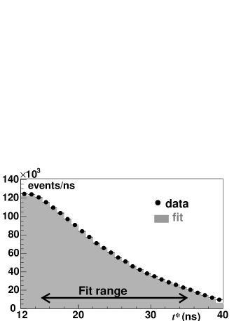
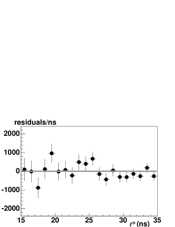
Figure 4: Decay length method. Left: fit to the $K^{+}$ proper time distribution: the black dots are data distribution, in grey the expected histogram fitting function. Right: Residuals in the region between 15 and 35 ns.

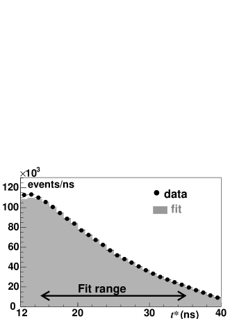
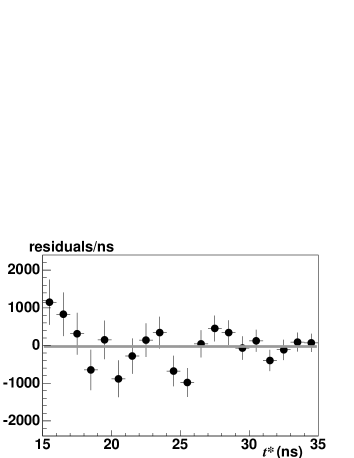
Figure 5: Decay length method. Left: fit to the $K^{-}$ proper time distribution: the black dots are data distribution, in grey the expected histogram fitting function. Right: Residuals in the region between 15 and 35 ns.

The measurements obtained for the two charges are in agreement with each other. Their weighted mean is:

$$\tau=(12.364\pm 0.031)~{}\rm{ns}.$$ (15)

6.2 Kaon decay time results

For the second method we build the expected histogram in the region between 10 and 50 ns. We made the fit in the region between 13 and 42 ns. The result from the fit to the $K^{+}$ proper decay time distribution, see fig. 6, is:

$$\tau^{+}=(12.315\pm 0.042)~{}\rm{ns}\hskip 28.45274pt\chi^{2}/\rm{ndf}=25.5/27\hskip 28.45274ptP(\chi^{2})=49\%.$$ (16)

For the $K^{-}$ lifetime, see fig. 7, we obtained:

$$\tau^{-}=(12.360\pm 0.043)~{}\rm{ns}\hskip 28.45274pt\chi^{2}/\rm{ndf}=22.9/27\hskip 28.45274ptP(\chi^{2})=69\%.$$ (17)

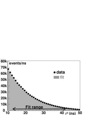
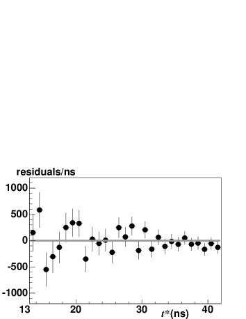
Figure 6: Decay time method. Left: fit to the $K^{+}$ proper time distribution: the black dots are data distribution, in grey the expected histogram fitting function. Right: Residuals in the region between 13 and 42 ns.

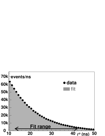
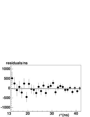
Figure 7: Decay time method. Left: fit to the $K^{-}$ proper time distribution: the black dots are data distribution, in grey the expected histogram fitting function. Right: Residuals in the region between 13 and 42 ns.

The measurements obtained for the two charges are in agreement with each other. Their weighted mean is:

$$\tau=(12.337\pm 0.030)~{}\rm{ns}.$$ (18)

As shown in the fig. 4, 5, 6 and 7 the agreement between data distribution and $\it{expected}$ histo distribution is very good also outside the fit range for both the charges and both the methods.

7 Systematic uncertainties

All the measurement strategy has been designed in order to have redundancy to keep systematic effects under control, and also to use as much as possible control samples selected on data, rather than relying on MonteCarlo simulations, for all the inputs to the fit. The determination of efficiencies has been already discussed; the efficiency correction effect has been checked by performing the fit with and without it. For the resolution functions, which at first order we obtain from MonteCarlo, we have checked the data/MC agreement on the distribution of the difference between the $t^{*}$ from the decay length and the $t^{*}$ from the decay time, on doubly reconstructed events. This allows us to check also the amount of incorrect bunch crossing determinations since the length is clearly not affected by this feature. The core of the time resolution is also kept under control by comparing the time of the two neutral clusters. All checks have shown very small data/MC corrections and negligible variations to the fit results and quality. The stability of the fit procedure with respect to the fit range has been checked by varying significantly the fit window and by changing the bin size from 1 ns to 0.5 or 2 ns. The systematics due to the selection have been obtained by comparing the fit results with different cuts for both the signal and the control samples. The beam pipe and DC wall thickness are known to about 10$\%$; this in turn affects the evaluation of the kaon energy loss in the materials and consequently the kaon $\beta$. We have repeated both measurements considering different thicknesses (by varying them within their errors) in order to assess the systematic effect on the lifetime. The energy loss inside the DC is more than one order of magnitude smaller than the one in the walls and the uncertainty on the material crossed inside the DC gives a negligible contribution to the systematic error on the lifetime measurements. The first method is very sensitive to systematic shift on the $\beta$ of the kaon (see eq. 4) and we observe a sizeable effect on the lifetime. This is not true for the second method (see eq. 10): for a typical charged kaon in our detector $\delta\gamma/\gamma\simeq 0.06\times\delta\beta/\beta$ and $t_{cl}$ depends on the kaon energy loss only at second order, via the third term of the $\chi^{2}$ function in eq. 7. For the time method the overall systematic effect due to the uncertainty on the kaon energy loss has been actually found negligible. The estimates of the systematic effects are summarized in table 1. The systematics of the two measurements are almost completely uncorrelated.

systematic uncertainty	Length (ps)	Time (ps)
Fit range	$\pm$ 10	$\pm$ 10
binning	$\pm$ 10	$\pm$ 10
efficiency correction	$\pm$ 15	$\pm$ 10
beam pipe thickness	$\pm$ 10	negligible
DC wall thickness	$\pm$ 15	negligible
Signal selection cuts	$\pm$ 15	negligible
Control sample cuts	negligible	$\pm$10
Resolution effects	negligible	negligible
total systematic uncertainty	$\pm$ 31	$\pm$ 20

Table 1: Sources of systematic uncertainties.

The result from the length measurement is:

$$\tau=(12.364\pm 0.031_{\rm{stat}}\pm 0.031_{\rm{syst}})~{}\rm{ns}$$ (19)

and from the time measurement is:

$$\tau=(12.337\pm 0.030_{\rm{stat}}\pm 0.020_{\rm{syst}})~{}\rm{ns}$$ (20)

8 Correlation and average

In order to average the two methods we calculate the statistical correlation between the two results. The correlation arises because the data samples used for the two methods have $\approx 30\%$ of events in common. The normalized correlation is 30.7$\%$ in agreement with a direct estimate obtained dividing the data in subsamples. Assuming that the systematic uncertainties are uncorrelated we then obtain the average:

$$\tau=(12.347\pm 0.030)~{}\rm{ns}$$ (21)

The measurement obtained agrees, within the errors, with the result given by Ott and Pritchard, [3]:

$$\tau=(12.380\pm 0.016)~{}\rm{ns}$$ (22)

and with the PDG fit, [4]:

$$\tau=(12.384\pm 0.024)~{}\rm{ns}$$ (23)

9 CPT test

The comparison of $K^{+}$ and $K^{-}$ lifetimes is a test of $CPT$ invariance which requires the equality of the decay lifetimes for particle and antiparticle. The average of the two methods is:

$$\begin{split}\tau^{+}=(12.325\pm 0.038)~{}\rm{ns}\\ \tau^{-}=(12.374\pm 0.040)~{}\rm{ns}\end{split}$$ (24)

From these measurements, and taking into account that most of the systematic effects cancel out in the ratio, we obtain:

$$\frac{\tau^{-}}{\tau^{+}}=1.004\pm 0.004$$ (25)

Our result agrees with $CPT$ invariance at the 0.4$\%$ level. Ref [10] had already verified agreement at the 0.08$\%$ level.

References

- [1] F. Ambrosino et al., [KLOE collaboration] Phys. Lett. B, 626:15-23, 2005
- [2] F. Ambrosino et al., [KLOE collaboration] Phys. Lett. B, 632:43-50, 2006
- [3] R. J. Ott T. W. Pritchard Phys.Rev. D3:52-56 1971.
- [4] W.-M. Yao et al., Journal of Physics, G33, 1 (2006)
- [5] S. Guiducci et al., Proc. of the 2001 Particle Accelerator Conference (Chicago, Illinois,(USA)), P. Lucas S. Webber Eds. 2001 353.
- [6] M. Adinolfi et al., [KLOE Collaboration], Nucl. Instrum. Meth A 488 2002 51
- [7] M. Adinolfi et al., [KLOE Collaboration], Nucl. Instrum. Meth A 482 2002 364
- [8] M. Adinolfi et al., [KLOE Collaboration], Nucl. Instrum. Meth A 492 2002 134
- [9] F. Ambrosino et al., [KLOE Collaboration], Nucl. Instrum. Meth A 534 2004 403
- [10] F. Lobkowicz et al., Phys.Rev. 185:1676-1687 1969
-
[11]
F. Ambrosino, P. Massarotti, Measurement of
charged Kaon lifetime, KLOE Note 218.
URL: http://www.lnf.infn.it/kloe/pub/knote/kn218.ps.