Quantum Dimer Model on the triangular lattice: Semiclassical and variational approaches to vison dispersion and condensation

Abstract

After reviewing the concept of vison excitations in $\mathbb{Z}_{2}$ dimer liquids, we study the liquid-crystal transition of the Quantum Dimer Model on the triangular lattice by means of a semiclassical spin-wave approximation to the dispersion of visons in the context of a “soft-dimer” version of the model. This approach captures some important qualitative features of the transition: continuous nature of the transition, linear dispersion at the critical point, and $\sqrt{12}\times\sqrt{12}$ symmetry-breaking pattern. In a second part, we present a variational calculation of the vison dispersion relation at the RK point which reproduces the qualitative shape of the dispersion relation and the order of magnitude of the gap. This approach provides a simple but reliable approximation of the vison wave functions at the RK point.

I Introduction

Since they have been shown to possess Resonating Valence Bond (RVB) phases on the triangular,ms01b kagomemsp02 and other (non-bipartite) lattices,ms03 Quantum Dimer Models (QDM) have been one of the main paradigms in the field of quantum spin liquids. These models, where the Hilbert space is spanned by hard-core dimer coverings of the lattice, are expected to capture the phenomenology of quantum antiferromagnets where the wave function is dominated by short-range valence bond configurations. On the triangular lattice, the simplest QDM is defined by the Hamiltonian:

$$\mathcal{H}= -t \sum_{r}\left(\left|\begin{picture}(22.0,10.0)(-8.0,-6.0) \put(-6.0,-10.0){\circle*{4.0}}\put(6.0,-10.0){\circle*{4.0}}\put(0.0,0.0){\circle*{4.0}}\put(12.0,0.0){\circle*{4.0}} \put(6.0,-10.0){\line(3,5){6.0}}\put(0.0,0.0){\line(-3,-5){6.0}} \end{picture}\right>\left<\begin{picture}(22.0,10.0)(-8.0,-6.0) \put(-6.0,-10.0){\circle*{4.0}}\put(6.0,-10.0){\circle*{4.0}}\put(0.0,0.0){\circle*{4.0}}\put(12.0,0.0){\circle*{4.0}} \put(-6.0,-10.0){\line(1,0){12.0}}\put(12.0,0.0){\line(-1,0){12.0}} \end{picture}\right|+{\rm H.c.}\right)$$ (1)

$$+V \sum_{r}\left(\left|\begin{picture}(22.0,10.0)(-8.0,-6.0) \put(-6.0,-10.0){\circle*{4.0}}\put(6.0,-10.0){\circle*{4.0}}\put(0.0,0.0){\circle*{4.0}}\put(12.0,0.0){\circle*{4.0}} \put(6.0,-10.0){\line(3,5){6.0}}\put(0.0,0.0){\line(-3,-5){6.0}} \end{picture}\right>\left<\begin{picture}(22.0,10.0)(-8.0,-6.0) \put(-6.0,-10.0){\circle*{4.0}}\put(6.0,-10.0){\circle*{4.0}}\put(0.0,0.0){\circle*{4.0}}\put(12.0,0.0){\circle*{4.0}} \put(6.0,-10.0){\line(3,5){6.0}}\put(0.0,0.0){\line(-3,-5){6.0}} \end{picture}\right|+\left|\begin{picture}(22.0,10.0)(-8.0,-6.0) \put(-6.0,-10.0){\circle*{4.0}}\put(6.0,-10.0){\circle*{4.0}}\put(0.0,0.0){\circle*{4.0}}\put(12.0,0.0){\circle*{4.0}} \put(-6.0,-10.0){\line(1,0){12.0}}\put(12.0,0.0){\line(-1,0){12.0}} \end{picture}\right>\left<\begin{picture}(22.0,10.0)(-8.0,-6.0) \put(-6.0,-10.0){\circle*{4.0}}\put(6.0,-10.0){\circle*{4.0}}\put(0.0,0.0){\circle*{4.0}}\put(12.0,0.0){\circle*{4.0}} \put(-6.0,-10.0){\line(1,0){12.0}}\put(12.0,0.0){\line(-1,0){12.0}} \end{picture}\right|\right)$$

where the sum runs over all plaquettes (rhombi) including the three possible orientations. The kinetic term, controlled by $t$, flips the two dimers on every flippable plaquette, i.e., on every plaquette with two parallel dimers, while the potential term controlled by the interaction $V$ describes a repulsion ($V>0$) or an attraction ($V<0$) between nearest-neighbor dimers.

The RVB phase is now relatively well understood. The first result goes back to Rokhsar and Kivelsonrk88 who showed that, for $V/t=1$ (the Rokhsar-Kivelson or RK point), the ground state is the sum of all configurations with equal amplitudes:

$$|RK\rangle=\frac{1}{\sqrt{\mathcal{N}}}\sum_{c}|c\rangle.$$ (2)

Since then, dimer-dimer correlations have been shown to be short-ranged in a range of parameters below $V/t=1$, ms01b ; ioselevich02 and the excitation spectrum to be gapped.ms01b ; ivanov04 ; ralko05 ; lca07 Besides, it has topologically degenerate ground states on non-simply connected clusters.ms01b ; ioselevich02 ; ralko05 This degeneracy is not related to a standard symmetry breaking. Indeed, there is no local order parameter,ioselevich02 ; fmo06 but only $\mathbb{Z}_{2}$ topological order.fm07

In QDM, the nature of the phase transition from a liquid to a solid is a long standing problem. It goes back to Jalabert and Sachdevjs91 (see also sv00 ) who studied a three-dimensional frustrated Ising model related to the square lattice QDM.

In a more general context, Senthil and Fishersf00 ; sf01 showed that models of Mott insulators can be cast in the form of a $\mathbb{Z}_{2}$ gauge theory. In this language, the transition from a fractionalized insulator to a conventionally ordered insulator appears to be a condensation of $\mathbb{Z}_{2}$-vortices (dubbed visons). Using a duality relation,wegner71 they showed that such transitions correspond to an ordering transition in a frustrated Ising model in transverse field. As we will see, this applies to the present QDM.

Building on a mapping between QDM’s at $V=0$ and Ising models in a transverse field, Moessner et al. msc00 ; ms01 have developed a Landau-Ginzburg approach and suggested that the transition could be continuous and in the three-dimensional $O(4)$ universality class.

Numerical evidence in favor of this scenario has been obtained with Green’s function Quantum Monte Carlo by Ralko et al., who have shown that, at the transition point, the static form factor of the crystal decreases to zero on the crystal side of the transition, while the dimer gap also decreases to zero on the liquid side.ralko06 More recently, the vison spectrum has also been numerically determined using Green’s function Quantum Monte Carlo, with the conclusion that a soft mode indeed develops at the transition.ralko07

In spite of these results, a simple picture for the wave functions of the visons and the evolution of their spectrum is still missing. One difficulty is that, like any vortex, these excitations cannot be created by operators which are local (in the dimer variables). To attack this problem, we follow two strategies. First of all, we look at the problem in the context of a $\mathbb{Z}_{2}$ gauge theory on the triangular lattice. As usual, this theory can be mapped onto a dual Ising model.wegner71 The duality transforms the nonlocal excitations of the gauge theory into local excitations, which we study using a semiclassical approach. This simple $1/S$ expansion already captures most aspects of the confinement-deconfinement transition (soft mode and condensation) of the $\mathbb{Z}_{2}$ gauge theory. Secondly, building on the explicit form of the excitations of the $\mathbb{Z}_{2}$ gauge theory, we construct single vison wave functions for the QDM and study the properties of the system at the RK point in the variational Hilbert space spanned by these states. These “variational visons” – living on the triangular plaquettes and experiencing a flux $\pi$ emanating from each site of the lattice – turn out to be linearly independent. The associated dispersion is in good qualitative agreement with that obtained in Monte Carlo simulations and the value of the gap at the RK point ($\Delta_{\rm var}=0.119$), obtained with a single variational parameter, has the correct order of magnitude (Monte Carlo simulationsivanov04 give 0.089). Improving quantitatively further these variational results would require more adjustable parameters to account in more details for the local (dimer-dimer, etc) correlations in the vicinity of the core of the vortex, a task which has not been carried out here.

II Visons in $\mathbb{Z}_{2}$ gauge theory

The connection between QDMs and $\mathbb{Z}_{2}$ gauge theories has already been discussed from different perspectives (see in particular Refs. sv00, ; msf02, ; msp02, ; ms03, ), and is rooted in the existence, in both families of models, of Ising-like degrees of freedom subjected to local constraints (hard-core constraints for the dimers, Gauss law for the gauge theory).

In this section, we review two known mappings: i) from a $\mathbb{Z}_{2}$ lattice gauge theory on the hexagonal lattice to the triangular lattice QDM (valid in a particular limit, Sec. II.1) and ii) from the $\mathbb{Z}_{2}$ theory to its dual frustrated Ising model (Sec.II.2). The latter Ising model is then studied using a semiclassical approximation in Secs. II.2.2 and II.2.3. Since the $\mathbb{Z}_{2}$ gauge theory - QDM mapping is formally justified only in the confined phase of the gauge theory, the relevance of the results obtained in the RVB (deconfined) phase of the QDM is not guaranteed a priori. Some reasons why this is expected to be the case are discussed in the next section, when we build on the results obtained for the excitations of the $\mathbb{Z}_{2}$ gauge theory in its deconfined phase to construct elementary excitations in the RVB phase of the QDM.

II.1 $\mathbb{Z}_{2}$ gauge theory

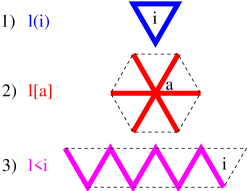
Figure 1: (Color online) Some useful definitions of sets of bonds: 1) $l(i)$ is the set of the three bonds forming the edges of the plaquette $i$. 2) $l[a]$ is the set of the six (fat) bonds emanating from the triangular site $a$. 3) $l<i$ denotes the bonds forming a “zigzag” string extending (to the left) from the triangular plaquette $i$ to an edge of the lattice.

To write down a $\mathbb{Z}_{2}$ gauge theory analogous to a QDM, the starting point is to define Pauli matrices $\vec{\tau}_{l}$ on the bonds $l$ of the triangular lattice such that $\tau^{x}_{l}=-1$ if bond $l$ is occupied by a dimer and $+1$ if it is empty, while $\tau^{z}_{l}$ changes the state of bond $l$. Since each kinetic term of the QDM flips the dimers around a rhombus, it corresponds to a product of four $\tau^{z}_{l}$ around this rhombus. This would, however, not keep the structure of the simple $\mathbb{Z}_{2}$ gauge theories, in which the kinetic term acts on an elementary plaquette of the lattice, a crucial ingredient to get a simple Ising model by duality.wegner71 An alternative is to consider the more standard $\mathbb{Z}_{2}$ gauge theory which, in its Hamiltonian formulation, is defined by:

$$H=H_{J}+H_{\Gamma}=-J\sum_{l}\tau^{x}_{l}-\Gamma\sum_{i}\prod_{l(i)}\tau^{z}_{l(i)};$$ (3)

where $i$ runs over the sites of the dual honeycomb lattice, and $l(i)$ are the three bonds forming the triangular plaquette around site $i$ (see Fig. 1). The hallmark of this model is to have local conserved quantities. Indeed,

$$[H,\prod_{l[a]}\tau^{x}_{l[a]}]=0,$$ (4)

where $a$ is a site of the triangular lattice, and the product over $l[a]$ runs over the six links emanating from $a$ (see Fig. 1). This allows one to define different sectors according to whether $\prod_{l[a]}\tau^{x}_{[a]}$ is equal to $+1$ or $-1$. Since in the QDM the number of dimers emanating from a given site is exactly equal to 1, it is clearly better to consider the sector where

$$\prod_{l[a]}\tau^{x}_{l[a]}=-1$$ (5)

for all $a$ since this forces the number of dimers emanating from a site to be odd (defining an odd Ising gauge theory in the terminology of Ref. msf02, ). Then, the true constraint is recovered in the limit $\Gamma/J\rightarrow 0$ if $J>0$ since, in the ground state, the number of dimers is then minimal. A bona fide QDM is then recovered if $H_{\Gamma}$ is treated with degenerate perturbation theory. Since $H_{\Gamma}$ changes the number of dimers, its effect vanishes to first order. To second order however, one recovers exactly the QDM of Eq. (1) with $V=0$ and $t=\Gamma^{2}/J$. So, if $J/\Gamma\gg 1$, the $\mathbb{Z}_{2}$ gauge theory maps onto the QDM at $V/t=0$. At finite $J/\Gamma$ the model can be viewed as a “soft-dimer” model, where 1, 3 or 5 dimers may touch a given site.

As we shall see below, the limit $J/\Gamma\gg 1$ lies deep inside the confined phase of the gauge theory, and from previous work on the QDM, it is known that at $V/t=0$, the model is in a Valence Bond Crystal phase. It would, of course, be very interesting to connect the two models away from this limit, when the gauge theory is in its deconfined phase and the QDM is in the dimer liquid phase. An interesting step in this direction is provided by higher order perturbation theory. Indeed, to fourth order in $\Gamma/J$, a repulsion between dimers $V=\Gamma^{4}/2J^{3}$ is generated. However, other terms of the same order, involving dimer shifts along loops of length 6, are also generated (see Appendix A). So, a rigorous mapping does not extend beyond the $V/t=0$ point.

II.2 Dual Ising model

As usual, this $\mathbb{Z}_{2}$ gauge theory is best analyzed by mapping it onto a dual Ising model in a transverse field.

II.2.1 The model

This can be achieved by introducing spin-$\frac{1}{2}$ operators $\vec{\sigma}_{i}$ on the dual honeycomb lattice:

$$\sigma^{x}_{i}=\prod_{l(i)}\tau^{z}_{l(i)},\ \ \sigma^{z}_{i}=\prod_{l<i}\tau^{x}_{l},$$ (6)

where $l<i$ represents all bonds cutting a straight path (say, horizontal, see Fig. 2 or 1) starting at $i$ (we implicitly assume a finite lattice with open boundary conditions). Combined with the constraint, this definition implies that

$$\sigma^{z}_{i}\sigma^{z}_{j}=M_{ij}\;\tau^{x}_{l}$$ (7)

for two neighboring sites $i,j$ separated by the bond $l$. $M_{ij}=\pm 1$ is such that each hexagon has exactly one $M_{ij}=-1$ bond (see Fig. 3). In terms of these spin operators, the Hamiltonian is the fully frustrated Ising model (FFIM)villain77 discussed by Moessner and Sondhi:ms01 ^,

$$H=H_{J}+H_{\Gamma}=-J\sum_{\langle i,j\rangle}M_{ij}\sigma^{z}_{i}\sigma^{z}_{j}-\Gamma\sum_{i}\sigma^{x}_{i}.$$ (8)

Note that choosing other paths to define $\sigma^{z}_{i}$ leads to other signs for $M_{ij}$, which, however, are always such that an odd number of minus signs appear around each hexagon, leading to the same Ising model up to a gauge transformation. The present choice leads to the smallest unit cell (4 honeycomb sites).

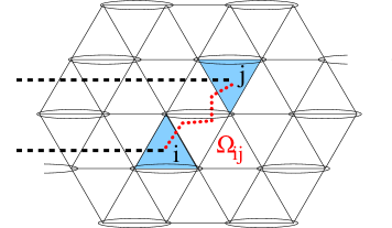
Figure 2: (Color online) Dashed lines: Horizontal paths used in Eq. 6 connecting the boundary of the system to triangles $i$ and $j$. Dotted segment: Path $\Omega_{ij}$. In this example $\Omega_{ij}$ crosses one dimer of the reference configuration $c_{0}$ (ellipses) and, therefore, $\epsilon_{ij}=-1$ (Eq. 58)

In the following, we study the phase diagram and the excitations of this model within a semiclassical (large $S$) approximation.

II.2.2 Classical phase diagram

First, we determine the classical ground state of the model as a function of $\Gamma/J$. To this end, we replace the spin-$\frac{1}{2}$ operators by classical 3-component vectors of unit length. Since the $y$ component does not appear in the Hamiltonian, it is clear that in the ground state the magnetization must lie in the $x$-$z$ plane. To find the lowest energy solution, we use the following parametrization:

$$\sigma^{z}_{i} \to \rho(i),$$ (9)

$$\sigma^{x}_{i} \to \sqrt{1-\rho(i)^{2}},$$ (10)

with $|\rho(i)|\leq 1$. The corresponding energy is

$$E=-\frac{J}{2}\sum_{ij}M_{ij}\rho(i)\rho(j)-\Gamma\sum_{i}\sqrt{1-\rho(i)^{2}}.$$ (11)

Initially defined for nearest neighbors (Eq. 7), the coefficients $M_{ij}$ have been upgraded to a matrix $M$ by setting all other elements to 0. This matrix describes the motion of a particle on a honeycomb lattice with 4 sites per unit cell and a flux $\pi$ per hexagonal plaquette. It reduces to a 4$\times$4 matrix after Fourier transformation. The eigenvalues associated with the momentum $k=(k_{x},k_{y})$ arems01

$$m_{k}^{1,2,3,4}=$$

$$\pm\sqrt{3\pm\sqrt{2[3+\cos(2k_{x})-\cos(k_{x}+k_{y})+\cos(k_{x}-k_{y})]}}.$$

Likewise, we denote by $\rho$ the column vector of components $\{\rho_{i}\}$.

$\Gamma/J>\sqrt{6}$ For $\Gamma\gg J$, we expect the $\rho(i)$’s to be small (or zero). We can, therefore, expand Eq. 11 to quadratic order:

$$E=-\frac{J}{2}\rho^{t}M\rho+\frac{1}{2}\Gamma\rho^{t}\rho.$$ (12)

The largest eigenvalue of $M$ being $\sqrt{6}$, we find that, as long as $\Gamma/J>\sqrt{6}$, the energy is minimized by $\rho=0$ and all spins point in the $x$ direction.

$0<\Gamma/J\leq\sqrt{6}$ At $\Gamma/J=\sqrt{6}$, all the real eigenvectors of $M$ for the eigenvalue $\sqrt{6}$ (satisfying $|\rho_{i}|\leq 1$) minimize Eq. 12. Let us choose four complex vectors which form a basis of the subspace associated with the eigenvalue $\sqrt{6}$:ms01

$$v_{1}(x,y) = v_{3}^{*}=\left[\begin{array}[]{c}e^{5i\pi/12}/F\\ e^{-i\pi/6}/F\\ 1\\ e^{-i\pi/12}\end{array}\right]\exp\left(\frac{i\pi}{6}x+i\frac{\pi}{2}y\right),$$ (17)

$$v_{2}(x,y) = v_{4}^{*}=\left[\begin{array}[]{c}e^{i\pi/12}\\ e^{-5i\pi/6}\\ 1/F\\ e^{-5i\pi/12}/F\end{array}\right]\exp\left(i\frac{5\pi}{6}x+i\frac{\pi}{2}y\right),$$ (22)

$$F = 2\sin(5\pi/12),$$ (23)

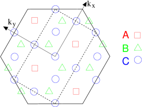
Figure 6: (Color online) Dashed rectangle: Brillouin zone ($-\pi\leq k_{x}\leq\pi$ and $-\pi\leq k_{y}\leq\pi$) of the hexagonal lattice shown in Fig. 3. A, B, and C are the high-symmetry points used in Fig. 5. The large hexagon is the Brillouin zone of the underlying triangular lattice.

where the 4 entries of the vector refer to the 4 sites in the unit cell (numbered as in Fig. 3) and $x,y$ are the (Bravais) coordinates of the unit cell. These eigenvectors correspond to the four points labelled B in the rectangular Brillouin zone of Fig. 6.

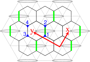
Figure 3: (Color online) The fat (green) bonds of the hexagonal lattice (crossed by a dimer of the reference configuration on the triangular lattice) have $M_{ij}=-1$, the other bonds have $M_{ij}=1$. The four sites of the unit cell (small blue triangles) are labelled from 1 to 4 and the Bravais vector are $x$ and $y$.

The most general real eigenvector $\rho$ can be parametrized by three angles $\alpha_{1}$, $\alpha_{2}$, and $\beta$ and a normalization factor $\lambda$:

$$\rho(i)=\lambda\left[\cos(\beta)\Re(v_{1}(i)e^{i\alpha_{1}})+\sin(\beta)\Re(v_{2}(i)e^{i\alpha_{2}})\right].$$ (24)

To find the ground state, the energy has to be minimized as a function of these 3 parameters. The analysis is made easier when one realizes that the second and fourth moments of the spin deviations are independent of the three angles. Indeed,

$$\frac{1}{N}\sum_{i}\rho(i)^{2} = r^{2}\lambda^{2},$$ (25)

$$\frac{1}{N}\sum_{i}\rho(i)^{4} = 2r^{4}\lambda^{4},$$ (26)

$${\rm with}\;\;r^{2} = \frac{1}{4}\left(1+\frac{1}{F^{2}}\right).$$ (27)

Replacing $\rho$ by Eq. 24 in the expression for the energy (Eq. 11), we get up to order $\lambda^{4}$:

$$E/N=-\Gamma+\frac{1}{2}\left(\Gamma-J\sqrt{6}\right)r^{2}\lambda^{2}+\frac{1}{4}\Gamma r^{4}\lambda^{4}+\mathcal{O}(\lambda^{6})$$ (28)

Minimizing with respect to $\lambda^{2}$ gives:

$$\lambda^{2}=\frac{J\sqrt{6}-\Gamma}{f^{2}\Gamma}.$$ (29)

For $\Gamma>J\sqrt{6}$ the energy is minimized for $\lambda=0$. For $\Gamma\leq J\sqrt{6}$, we have to expand Eq. 11 to the 6^th order to find the angles $\alpha_{1}$, $\alpha_{2}$ and $\beta$ which minimize the classical energy. Indeed, Eq. 28 shows that, up to order $\lambda^{4}$, the energy is independent of the three angles. At this order, the energy is constant and minimum on a 3-dimensional sphere, a consequence of the $O(4)$ symmetry discovered by Moessner and Sondhi.ms01 One, therefore, has to go to the next order to find the actual minima. At 6^th order in $\lambda$, the energy is minimized when

$$\frac{1}{N}\sum_{i}\rho(i)^{6}$$ (30)

is minimum. A numerical investigation shows that the solutions (for $\Gamma/J$ close to but below $\sqrt{6}$) are 48-fold degenerate and can be deduced from each other by symmetry operations (12 translations and 4 point-group operations). This confirms the result obtained previously on symmetry grounds.msc00 ; ms01

Motivated by the FFIM/dimer model correspondence, we are interested in the average “dimer density”:

$$d_{ij}=\frac{1}{2}(1-M_{ij}\langle\sigma^{z}_{i}\sigma^{z}_{j}\rangle)$$ (31)

for all pairs $(i,j)$ of nearest-neighbor honeycomb sites. In the classical limit, this may be approximated by

$$d_{ij}=\frac{1}{2}(1-M_{ij}\rho(i)\rho(j)),$$ (32)

where $\rho$ (Eq. 24) is the classical ground state. Close to the transition at $\Gamma_{c}=J\sqrt{6}$, $\rho$ scales as $\lambda\sim\sqrt{\Gamma_{c}-\Gamma}$ (Eq. 29) and the “dimer density”, thus, shows small deviations about $\frac{1}{2}$. To visualize the “dimerization” pattern in the vicinity of $\Gamma_{c}$, the appropriate quantity is, therefore, a relative rescaled “dimer” density defined by $D_{ij}=\frac{1}{\lambda^{2}}(d_{ij}-\frac{1}{2})$, and plotted in Fig. 4 for one of the 48 ground states. The obtained pattern is highly reminiscent of the $\sqrt{12}\times\sqrt{12}$ VBC observed in the triangular lattice QDM. In particular, the 48 spin configurations give only 12 different “dimer” patterns, with a smaller unit cell containing 12 sites of the triangular lattice. It is also interesting to notice that $\rho(i)$ vanishes in the triangles located inside the large diamonds (marked with a dot in Fig. 4). From Eq. 10, the corresponding sites have a magnetization pointing exactly in the $x$ direction, which means a total absence of “vison” and local correlations identical to that of the $J=0$ paramagnetic ground state. The “dimer” density $d_{ij}$ is uniform inside these diamonds, in qualitative agreement with the intriguing observation made in Ref. ralko06, .

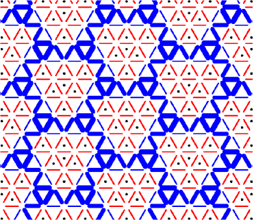
Figure 4: (Color online) Plot of the rescaled relative “dimer” density $D_{ij}$ in one of the 48 classical ground states of the FFIM in transverse field, for a transverse field $\Gamma$ just below $\Gamma_{c}$. Thin red bonds represent $D_{ij}=0$ (corresponding to the highest “dimer density” $d_{ij}=0.5$). Blue bonds are for $D_{ij}<0$, that is, a lower dimer density, with a width proportional to $|D_{ij}|$. $D_{ij}$ takes only 4 different values: 0, -0.259, -0.518, and -0.776.

II.2.3 Semi-classical analysis for $\Gamma/J\geq\sqrt{6}$

If $J=0$, the ground state is the fully polarized state $\sigma^{x}_{i}=1$. The first (degenerate) excited state is obtained by flipping one spin at some arbitrary triangle. To first order in $J/\Gamma$, the spectrum is obtained by diagonalizing the perturbation $H_{J}$ in this subspace. This amounts to diagonalizing $M$, and leads to the eigenvalues $\epsilon^{i}_{k}=2\Gamma+Jm^{i}_{k}$, a result already obtained previously.ms01

To go further, beyond the limit $J/\Gamma\ll 1$, we perform a $1/S$ semiclassical expansion. We generalize the spin-1/2 Hamiltonian to an arbitrary value $S$ of the spin:

$$\mathcal{H}=-\frac{J}{S^{2}}\sum_{\langle i,j\rangle}M_{ij}S^{z}_{i}S^{z}_{j}-\frac{\Gamma}{S}\sum_{i}S^{x}_{i}$$ (33)

(which reduces to Eq. 8 when $S=1/2$). Spin deviations away from the $x$ directions are represented using Holstein-Primakoff bosons. To leading order in $1/S$:

$$S^{z}_{i} = \frac{1}{2}\sqrt{2S}\left(b^{\dagger}_{i}+b_{i}\right),$$ (34)

$$S^{x}_{i} = S-b^{\dagger}_{i}b_{i}.$$ (35)

One truncates the Hamiltonian to quadratic order in $b_{i}$, and diagonalizes it through a Bogoliubov transformation:

$$b^{\dagger}_{i} = \sum_{j}U_{ij}a^{\dagger}_{j}+\sum_{j}V_{ij}a_{j}$$ (36)

For the $a^{\dagger}_{j}$ operators to be bosonic creation operators, the matrices $U$ and $V$ must satisfy $U^{\dagger}U-V^{\dagger}V=1$. It is convenient to introduce a unitary matrix $\Omega$ which transforms $M$ into a diagonal matrix $\tilde{M}$:

$$M = \Omega\tilde{M}\Omega^{\dagger},$$ (37)

$$\tilde{M}_{kp} = m_{k}\delta_{kp}.$$ (38)

In this new basis, we can look for diagonal solutions for $U$ and $V$:

$$U=\Omega\tilde{U}\Omega^{\dagger}\;\;,\;\;V=\Omega\tilde{V}\Omega^{\dagger},$$ (39)

$$\tilde{U}_{kp}=u_{k}\delta_{kp}\;\;,\;\;\tilde{V}_{kp}=v_{k}\delta_{kp}.$$ (40)

Since $M$ is real, we can choose $\Omega\in O(N)$. After some algebra, one finds that the $u_{k}$ and $v_{k}$ which diagonalize $H$ are given by

$$u_{k} = \cosh(\theta_{k}),$$ (41)

$$v_{k} = \sinh(\theta_{k}),$$ (42)

$$\tanh(2\theta_{k}) = -\frac{m_{k}}{m_{k}+2\Gamma/J}.$$ (43)

The energies of the Bogoliubov excitations are given by

$$\epsilon_{k} = \frac{J}{S}\sqrt{\frac{\Gamma}{J}\left(m_{k}+\frac{\Gamma}{J}\right)}.$$ (44)

As expected, the spectrum becomes gapless at $\Gamma/J=\sqrt{6}$ and we recover the localized spin flip energy $\epsilon_{k}\simeq\Gamma/S$ when $\Gamma\to\infty$. The Bogoliubov spectrum is shown Fig. 5 for a few values of $\Gamma$ at or above $\Gamma_{c}$. One clearly sees that the dispersion is linear around the gapless points at the transition.

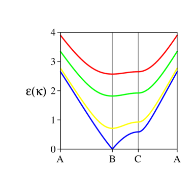
Figure 5: (Color online) Spin-wave dispersion relation $S\epsilon_{k}/J$ (Eq. 44) for the path A$\to$B$\to$C$\to$A in the Brillouin zone (see Fig. 6) and different values of $\Gamma/J$:3 (top), 2.75, 2.5, and $\sqrt{6}\simeq 2.448$ (bottom). At the critical point $\Gamma/J=\sqrt{6}$, the spectrum is linear around $k=(\pi/6,\pi/2)$ and $k=(5\pi/6,\pi/2)$.

This behavior is remarkably similar to that found numerically by Ralko et al.ralko07 for the QDM by Green’s function Quantum Monte Carlo. In the next section, we build on this resemblance to develop a variational approach to the vison spectrum of the QDM. Note that, as stated above, the $\mathbb{Z}_{2}$ gauge theory and the QDM can only be rigorously mapped onto each other deep into the confined (resp. VBC) phase, and the resemblance between their spectra in the deconfined (resp. RVB) phases might seem fortuitous. A somewhat deeper connection will be described in the next section.

III Visons in the Quantum Dimer Model

In the Ising model, elementary excitations for large enough $\Gamma/J$ are spin flips, induced by $\sigma^{z}_{i}$, which delocalize and get dressed under the effect of $H_{J}$. In the equivalent dual gauge theory, this excitation is produced by the nonlocal string operator $\sigma^{z}_{i}=\prod_{l<i}\tau^{x}_{l}$. By analogy, it is natural to define a “point” vison creation operator for the QDM byrc89 ; ioselevich02

$$V_{i}=(-1)^{\hat{N}(i)}\;\;,\;\;\hat{N}(i)=\sum_{l<i}\hat{n}_{l},$$ (45)

where the dimer operator $\hat{n}_{l}$ is defined by $\hat{n}_{l}=1$ if bond $l$ is occupied, and $0$ otherwise. Again, we consider here a finite lattice with open boundary conditions. Let us first see to which extent this operator is the analog of the vortex creation operator in Ising gauge theories.

III.1 $\mathbb{Z}_{2}$ gauge structure of QDM

In gauge theories, the Wilson loop operator defined by

$$W_{\partial\Omega}=\prod_{l\in\partial\Omega}\tau^{z}_{l}$$ (46)

plays a central role since it allows one to distinguish (in the absence of matter field, as here) the deconfined and confined phases depending on whether its ground state expectation value (or flux) tends to zero exponentially with the perimeter of the domain $\Omega$ (deconfined) or with the area of the domain (confined). For a $\mathbb{Z}_{2}$ gauge theory $W_{\partial\Omega}^{2}=1$ and the flux going through $\Omega$ measured by $W_{\partial\Omega}$ can only take two values $\pm 1$. In that respect, an interesting property of the operator $\sigma^{z}_{i}=\prod_{l<i}\tau^{x}_{l}$ is that it changes the flux between -1 and +1 if the site $i$ is inside the domain. Then, $\sigma^{z}_{i}\sigma^{z}_{j}$ commutes with the Wilson loop and does not change the flux unless $i$ and $j$ sit on opposite sides of the boundary. Since the deconfined phase can be accessed from the $J\ll\Gamma$ limit, the ground state can be thought of as an Ising paramagnet ($\sigma^{x}=1$ and $W_{\partial\Omega}=1$ everywhere) “dressed” perturbatively by successive applications of $J\sigma^{z}_{i}\sigma^{z}_{j}$, where $i$ and $j$ are nearest neighbors. Since $J\sigma^{z}_{i}\sigma^{z}_{j}$ only changes the flux for pairs $ij$ across the boundary, the expectation value of the Wilson loop operator behaves according to a perimeter law. A similar perturbative argument can be used to derive the area law in the confined phase.

Most of these standard $\mathbb{Z}_{2}$ gauge theory results apply to the QDM, with one difficulty however. The Wilson loop operator cannot be defined in the same way since flipping the dimer occupation along a loop will often lead to an unphysical state that violates the condition of having exactly one dimer emanating from each site. Different ways to overcome this problem can be envisaged. One possibility is to accept that the Wilson loop operator gives zero when applied to states that are non-flippable along the loop. The property $W_{\partial\Omega}^{2}=1$ is lost, but $W_{\partial\Omega}$ has eigenvalues $0$, $+1$, or $-1$, and eigenstates with eigenvalues $+1$ or $-1$ are still interchanged when a vison operator (Eq. 45) is applied inside the domain. So confinement or deconfinement of visons is still expected to lead to area or perimeter laws.

Alternatively, starting from the observation that, when it does not give zero, the Wilson loop operator just shifts the dimers along the contour, one can try to define a (complicated) flux operator in the dimer space which shifts the dimer along a “fattened” contour which “adapts” locally to the dimer configuration it acts upon. Although tricky to define in practice, this operator would have the advantage that its square is still equal to 1, preserving the manifest $\mathbb{Z}_{2}$ structure of the theory.

Another way to underline the deep connection between the two models is to consider the Ising model as a “soft-dimer” model and introduce the projection operator onto the “hard-core” dimer Hilbert space, defined by:

$$\hat{P}=\prod_{p}\frac{(\hat{n}_{p}-3)(\hat{n}_{p}-5)}{(1-3)(1-5)}$$ (47)

where the operator $\hat{n}_{p}$ counts the number of frustrated bonds (dimers) around the plaquette $p$:

$$\hat{n}_{p}=\frac{1}{2}\sum_{i=1}^{6}(1-M_{i,i+1}\sigma^{z}_{i}\sigma^{z}_{i+1})$$ (48)

By construction, $\hat{P}=1$ on all the Ising configurations which correspond to a valid “hard-core” dimer covering (of the triangular lattice) and $\hat{P}=0$ otherwise. Now, $\hat{P}$ commutes with $\prod_{i}\sigma^{x}_{i}$ since all terms in $\hat{P}$ contain an even number of $\sigma^{z}$ operators. This means that $\hat{P}$ conserves the total flux, so that a spin state with -1 flux becomes a dimer wave function with an odd number of visons after projection.

III.2 Point vison

Equation 45 defines the simplest operator which changes the flux, that is, which creates a vison. So we may consider

$$|i\rangle = V(i)|RK\rangle=\frac{1}{\sqrt{\mathcal{N}}}\sum_{c}(-1)^{\hat{N}(i)}|c\rangle$$ (49)

$$= \frac{1}{\sqrt{\mathcal{N}}}\hat{P}\sigma^{z}_{i}|\left\{\sigma^{x}_{j}=+1\right\}\rangle$$ (50)

as a first variational approximation to the true lowest eigenstate of $\mathcal{H}$ in the $-1$ flux sector ($\mathcal{N}$ is the total number of dimer coverings). The ground state $|RK\rangle$ is a zero-energy eigenstate of $\mathcal{H}$, implying that the expectation value $E_{K}<0$ of the kinetic energy term exactly compensates the expectation value $E_{P}>0$ of the potential energy term. Indeed,

$$E_{P}=3Np_{0}=-E_{K},$$ (51)

where $3N$ is the total number of rhombi ($N$ the number of sites) and $p_{0}$ the probability to have 2 parallel dimers on a given rhombus in the classical dimer problem (with uniform measure over all dimer configurations). Using the Pfaffians method,k61 ; krauth one finds in the thermodynamic limit

$$p_{0}\simeq 0.0933310104...$$ (52)

In $|i\rangle$ the expectation value of the potential energy term is the same as in $|RK\rangle$. In fact, all the observables which are diagonal in the dimer basis commute with $\sigma^{z}$ and thus have the same expectation value in the ground state $|RK\rangle$ and in the trial wave function $|i\rangle$. The increase of the energy is only kinetic. Because the kinetic terms corresponding to the three diamonds around $i$ anticommute with $\sigma^{z}_{i}$, their expectation values has changed sign. Thus we find

$$\langle i|\mathcal{H}|i\rangle-\langle RK|\mathcal{H}|RK\rangle=6p_{0}\simeq 0.56.$$ (53)

III.3 Dispersing point vison

One can lower the energy by constructing plane waves. To compute the associated dispersion relation we have to evaluate the following matrix elements:

$$S_{ij}^{0} = \langle i|j\rangle$$ (54)

$$H_{ij}^{0} = \langle i|\mathcal{H}|j\rangle$$ (55)

We begin with the overlap matrix

$$S_{ij}^{0} = \frac{1}{\mathcal{N}}\sum_{c}\langle c|(-1)^{\hat{N}(i)+\hat{N}(j)}|c\rangle$$ (56)

($\hat{N}(i)$ and $\hat{N}(j)$ are defined in Eq. 45) which simplifies to

$$S_{ij}^{0} = \epsilon_{ij}\frac{1}{\mathcal{N}}\sum_{c}\langle c|(-1)^{\hat{N}(i,j)}|c\rangle$$ (57)

$$\epsilon_{ij} = (-1)^{N_{0}(i,j)}$$ (58)

where the local operator $\hat{N}(i,j)$ counts the number of dimers across some path $\Omega_{ij}$ connecting the triangles $i$ and $j$ (see Fig. 2), and $N_{0}(i,j)$ is equal to that number in the reference configuration $c_{0}$, chosen with all the dimers horizontal (Fig. 2). This follows from two simple properties: $\langle c|(-1)^{\hat{N}(i)+\hat{N}(j)+\hat{N}(i,j)}|c\rangle$ is independent of the configuration $c\rangle$, and $\langle c_{0}|(-1)^{\hat{N}(i)+\hat{N}(j)}|c_{0}\rangle=1$. We finally write

$$S_{ij}^{0}=\epsilon_{ij}\left<(-1)^{\hat{N}(i,j)}\right>$$ (59)

where $\left<\cdots\right>$ represents the average with equal weight over all dimer coverings.

The average of any such diagonal observable can be computed using the Pfaffian of a (modified) Kasteleyn matrix.k61 ; krauth In the present case, the “string” observable $(-1)^{\hat{N}(i,j)}$ is coded in the Kasteleyn matrix by changing the signs of the matrix elements corresponding to bonds crossed by $\Omega_{ij}$, i.e., setting some bond fugacities to $-1$. To evaluate numerically such an expectation value, we construct the modified Kasteleyn matrices corresponding to a large enough triangular lattice, in which the path $\Omega_{ij}$ is embedded. Finite-size effects decay exponentially with the system size, so that lattices with $28\times 28$ sites (with periodic boundary conditions) can safely be used to evaluate $S_{ij}^{0}$ with high accuracy up to distances $d\simeq 10$ between triangles $i$ and $j$.

The matrix elements $S_{ij}^{0}$, plotted in Fig. 7 as a function of the distance between $i$ and $j$, decay exponentially (a result anticipated by Read and Chakrabortyrc89 ). These quantities have already been evaluated by Ioselevich et al.ioselevich02 using a classical Monte Carlo sampling.

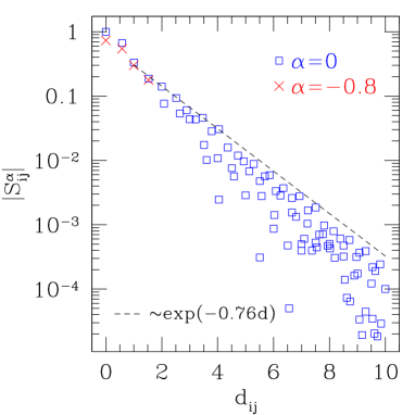
Figure 7: (Color online) Overlap $|\langle i|j\rangle|$ between two point-vison states (defined in Eq. 49) as a function the distance $d_{ij}$ between $i$ and $j$. The (blue) square correspond to Eq. 54 and the three (red) crosses correspond to Eq. 81 with $\alpha=-0.8$. The calculations are done using an exact evaluation of the Pfaffians on a $28$-site lattice with periodic boundary conditions. Dashed line: guide to the eye corresponding to an exponential decay with the dimer-dimer correlation length $\xi^{-1}=0.76$.ioselevich02

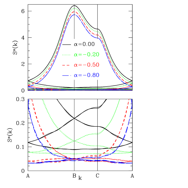
Figure 8: (Color online) Spectrum of the overlap matrix $S^{\alpha}(k)$ (Eqs.54 and 81), for different values of $\alpha$ (0, -0.2, -0.5 and -0.8), along the path A$\to$B$\to$C$\to$A in the Brillouin zone (see Fig. 6). The bottom panel is a zoom on the lowest eigenvalues of $S^{\alpha}$. In these calculations, the matrix elements $S_{ij}^{\alpha}$ are neglected for triangles $i$ and $j$ at distance $d\geq d_{\rm max}=10$ (102^th neighbor on the hexagonal lattice). Up to this distance, the finite-size lattice used in the calculation ($28\times 28$ sites) gives practically the infinite volume limit for $S_{ij}^{\alpha}$. The value of $d_{\rm max}$ used here is large enough to ensure a good convergence of the spectrum since the curves obtained with a smaller truncation distance ($d_{\rm max}\simeq 8.47$ – shown here with the same colors) are almost superposed with that for $d_{\rm max}=10$, except for the bottom of the spectrum at $\alpha=-0.5$ and $\alpha=-0.8$. The overlap spectrum turns out to be gapped for $\alpha=0$ and $\alpha=-0.2$ (and probably at $\alpha=-0.5$ and $\alpha=-0.8$ too), indicating the linear independence of the vison states.

By construction, a product like $\epsilon_{i_{1},i_{2}}\epsilon_{i_{2},i_{3}}\cdots\epsilon_{i_{n},i_{1}}$ (where $i_{1},i_{2},\cdots,i_{n}$ form a closed loop of triangles) is equal to the parity of the number of sites enclosed in the loop. Thus, the signs of the matrix elements $S_{ij}^{0}$ are similar to those of the hopping amplitude of a particle moving on the hexagonal lattice and subjected to a magnetic field corresponding to half a flux quantum per hexagon. In such a case, the magnetic unit cell has to be doubled compared to the original lattice cell. Since the original unit cell contains one triangular site and two triangular plaquettes, the magnetic one contains four triangular plaquettes and thus four sites of the hexagonal lattice. In Fourier space, $S^{0}(k)$ is a $4\times 4$ matrix, as the matrix $M$ discussed previously. The same is also true for the Hamiltonian matrix elements described below.

The spectrum of the overlap matrix $S^{0}(k)$ is plotted in Fig. 8 (for $k$ describing a representative path in the Brillouin zone). As an important result, the eigenvalues are strictly positive for all $k$. To our knowledge, it is the first time that the linear independence of point vison states is proved.

Let us now turn to the matrix elements of the Hamiltonian. We wish to transform Eq. 55 into an expression which can be evaluated using the Pfaffians, that is the expectation value of a diagonal observable in the dimer basis. First, we write $\mathcal{H}$ as a sum of projectors

$$\mathcal{H} = 2\sum_{r_{0}}\hat{\Pi}_{r_{0}}$$ (60)

$$\hat{\Pi}_{r_{0}} = |\psi_{r_{0}}\rangle\langle\psi_{r_{0}}|$$ (61)

$$|\psi_{r_{0}}\rangle = \frac{1}{\sqrt{2}}\left(\left|\begin{picture}(22.0,10.0)(-8.0,-6.0) \put(-6.0,-10.0){\circle*{4.0}}\put(6.0,-10.0){\circle*{4.0}}\put(0.0,0.0){\circle*{4.0}}\put(12.0,0.0){\circle*{4.0}} \put(-6.0,-10.0){\line(1,0){12.0}}\put(12.0,0.0){\line(-1,0){12.0}} \end{picture}\right>-\left|\begin{picture}(22.0,10.0)(-8.0,-6.0) \put(-6.0,-10.0){\circle*{4.0}}\put(6.0,-10.0){\circle*{4.0}}\put(0.0,0.0){\circle*{4.0}}\put(12.0,0.0){\circle*{4.0}} \put(6.0,-10.0){\line(3,5){6.0}}\put(0.0,0.0){\line(-3,-5){6.0}} \end{picture}\right>\right)$$ (62)

and expand Eq. 55 into

$$H_{ij}^{0} = \frac{2}{\mathcal{N}}\sum_{c_{1},c_{2}}\sum_{r_{0}}(-1)^{N(c_{1},i)+N(c_{2},j)}\langle c_{1}|\hat{\Pi}_{r_{0}}|c_{2}\rangle,$$ (63)

with the notation $N(c,i)=\langle c|\hat{N}(i)|c\rangle=\pm 1$. Because of the double sum $\sum_{c_{1},c_{2}}$, this does not yet have the form of a diagonal observable amenable to an evaluation with Pfaffians. To go further we note that $\langle c_{1}|\hat{\Pi}_{r_{0}}|c_{2}\rangle$ vanishes if $c_{1}$ and/or $c_{2}$ is not flippable around the rhombus ${r_{0}}$. In addition, $\langle c_{1}|\hat{\Pi}_{r_{0}}|c_{2}\rangle=0$ if $c_{1}$ and $c_{2}$ differ anywhere outside ${r_{0}}$. So we can restrict the sum to pairs of configurations $(c,\bar{c})$ which differ by a dimer flip in ${r_{0}}$ and which are identical elsewhere on the lattice:

$$H_{ij}^{0} = \frac{2}{\mathcal{N}}\sum_{r_{0}}\sum_{\begin{array}[]{c}(c,\bar{c})\\ F_{r_{0}}(c)=1\end{array}}$$ (67)

$$\left[(-1)^{N(c,i)}\langle c|+(-1)^{N(\bar{c},i)}\langle\bar{c}|\right]$$

$$\hat{\Pi}_{r_{0}}\left[(-1)^{N(c,j)}|c\rangle+(-1)^{N(\bar{c},j)}|\bar{c}\rangle\right]$$

where $F_{r_{0}}(c)=1$ if $c$ is flippable on rhombus ${r_{0}}$, and $F_{r_{0}}(c)=0$ otherwise.

$c$ and $\bar{c}$ only differ inside ${r_{0}}$, so the signs $(-1)^{N(c,i)}$ and $(-1)^{N(\bar{c},i)}$ are the same if $i$ is not inside $r_{0}$, and are opposite if $i\in{r_{0}}$. Let us note $\delta_{i,{r_{0}}}=-1$ if $i\in{r_{0}}$ and $\delta_{i,{r_{0}}}=1$ otherwise. This leads to

$$H_{ij}^{0} = \frac{2}{\mathcal{N}}\sum_{r_{0}}\sum_{\begin{array}[]{c}(c,\bar{c})\\ F_{r_{0}}(c)=1\end{array}}(-1)^{N(c,i)+N(c,j)}$$ (71)

$$\times\left[\langle c|+\delta_{i,{r_{0}}}\langle\bar{c}|\right]\hat{\Pi}_{r_{0}}\left[|c\rangle+\delta_{j,{r_{0}}}|\bar{c}\rangle\right].$$

Using the explicit form of $\hat{\Pi}_{r_{0}}$, we get

$$\left[\langle c|+\delta_{i,{r_{0}}}\langle\bar{c}|\right]\hat{\Pi}_{r_{0}}\left[|c\rangle+\delta_{j,{r_{0}}}|\bar{c}\rangle\right]=\frac{1}{2}(1-\delta_{i,{r_{0}}})(1-\delta_{j,{r_{0}}})$$

and, finally,

$$H_{ij}^{0} = \sum_{r_{0}}(1-\delta_{i,{r_{0}}})(1-\delta_{j,{r_{0}}})$$ (78)

$$\times\frac{1}{2\mathcal{N}}\sum_{\begin{array}[]{c}c\\ F_{r_{0}}(c)=1\end{array}}(-1)^{N(c,i)+N(c,j)}$$

$$= \epsilon_{ij}\sum_{r_{0}}(1-\delta_{i,r_{0}})(1-\delta_{j,{r_{0}}})$$

$$\times\frac{1}{2\mathcal{N}}\sum_{\begin{array}[]{c}c\\ F_{r_{0}}(c)=1\end{array}}\langle c|(-1)^{\hat{N}(i,j)}|c\rangle.$$

The last expression is the average of a diagonal observable and can, thus, be evaluated using Pfaffians:

$$H_{ij}^{0} = \frac{1}{2}\epsilon_{ij}\sum_{r_{0}}(1-\delta_{i,{r_{0}}})(1-\delta_{j,{r_{0}}})$$ (79)

$$\times\left<(-1)^{\hat{N}(i,j)}\hat{F}_{r_{0}}\right>$$

where we used an operator notation for the “flippability” $\hat{F}_{r_{0}}|c\rangle=F_{r_{0}}(c)|c\rangle$. To get a nonzero contribution, there must be at least one rhombus ${r_{0}}$ containing $i$ and $j$. So $H_{ij}^{0}=0$ if $i$ and $j$ are not nearest neighbors. Using modified Kasteleyn matrices in a way similar to that described for the overlap matrix $S^{0}$, the nonzero matrix elements can be calculated. We find $|H_{ij}^{0}|=6p_{0}$ for $i=j$, $|H_{ij}^{0}|=2p_{0}$ when $i$ and $j$ are first neighbors.

Although the matrix elements of $\mathcal{H}$ are simple, the band structure is, however, not that of a simple tight-binding Hamiltonian, because of the non-orthogonality of the present variational vison states. In Fourier space, $S^{0}(k)$ and $H^{0}(k)$ are $4\times 4$ matrices. The spectrum is obtained by solving the generalized eigenvalue problem $H^{0}(k)\psi_{k}-E(k)S^{0}(k)\psi_{k}=0$. The results are shown in Fig. 9 ($\alpha=0$ curve). The minimum of $\epsilon_{k}$ is found at $(k_{x},k_{y})=(\pi/6,\pi/2)$, in agreement with the Monte Carlo results.ivanov04 ; ralko06 The corresponding energy is $\epsilon_{\rm min}=0.16$, which is significantly lower than the energy (0.56) found above for a completely localized point vison $|i\rangle$. The bottom of this variational point vison band is, however, still high compared to Ivanov’sivanov04 estimate (0.089) of the gap in the vison sector. The next section provides an improved family of variational states.

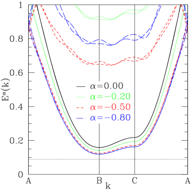
Figure 9: (Color online) Variational vison (Eq. 80) dispersion relation for different values of $\alpha$, along the path A$\to$B$\to$C$\to$A in the Brillouin zone (see Fig. 6). The curve for $\alpha=0$ corresponds to the variational energies of point-vison states (Eq. 49). The absolute minimum is $E_{\rm min}=0.119$, found at $(k_{x},k_{y})=(\pi/6,\pi/2)=B$ for a value $\simeq-0.8$ of the variational parameter $\alpha$. The exact value of the gap (0.089)ivanov04 is marked as a dotted horizontal line. In this calculation, the matrix elements $S_{ij}^{\alpha}$ are neglected for triangles $i$ and $j$ at distance $d\geq d_{\rm max}=10$. This value is large enough to ensure a perfect convergence of the spectrum below $E\lesssim 0.6$, as can be checked from the fact that the dispersion curves obtained with a smaller truncation distance ($d_{\rm max}\simeq 8.47$ – shown here with the same colors) are practically identical. Some higher energy states, however, are not fully converged.

III.4 Dressed vison

The vison wave function of Eq. 49, differs from the RK wave functions only through minus signs. It has the “accidental” property that dimer-dimer correlations are the same as in the ground state. As a consequence, the excitation energy of such a state is carried only by the kinetic part of the Hamiltonian. Clearly, some local reweighting of the dimer configurations in the vicinity of the vortex core would allow an optimized balance between the potential and kinetic costs of the excitation, and would lead to an improved variational wave function. This amounts to “dressing” locally the initial point-vison state by some even – but fluctuating – number of additional point visons.

As a simple improvement of the vison wave function, we introduce a variational parameter $\alpha$ to reweight the configurations depending on their “flipability” at the core of the vison. This gives the following vison state:

$$|i,\alpha\rangle = \frac{1}{\sqrt{\mathcal{N}}}\sum_{c}(-1)^{\hat{N}(i)}\left(1+\alpha\hat{F}_{i}\right)|c\rangle,$$ (80)

$$\hat{F}_{i} = \hat{F}_{r_{1}(i)}+\hat{F}_{r_{2}(i)}+\hat{F}_{r_{3}(i)},$$

where $\hat{F}_{i}|c\rangle=|c\rangle$ if the dimer configuration $c$ is flippable around one of the three rhombi $r_{1}(i)$, $r_{2}(i)$, and $r_{3}(i)$ containing the triangle $i$, and $\hat{F}_{i}|c\rangle=0$ otherwise.

As for the point vison of Eq. 49, the vison states of Eq. 80 are not orthogonal and we have to evaluate their overlaps:

$$S^{\alpha}_{ij}=\langle i,\alpha|j,\alpha\rangle$$ (81)

Repeating the transformation leading to Eq. 59, we get

$$S_{ij}^{\alpha}=\epsilon_{ij}\left<(-1)^{\hat{N}(i,j)}\left(1+\alpha\hat{F}_{i}\right)\left(1+\alpha\hat{F}_{j}\right)\right>,$$ (82)

which is an expectation value for a diagonal operator that we evaluate using Pfaffians. In addition to the sign changes due to $(-1)^{\hat{N}(i,j)}$, some entries of the Kasteleyn matrix have to be modified to incorporate the flippability operators $\hat{F}_{r}$. More precisely, counting only the coverings which satisfy $\hat{F}_{r}=1$ is done by “isolating” the rhombus $r$, that is, by switching to zero in the Kasteleyn matrix the 14 bonds which connect the sites of rhombus $r$ to their neighbors outside $r$.

Beyond some distance between the vison cores $i$ and $j$ (fourth neighbor on the hexagonal lattice), no rhombus can touch simultaneously both triangles. In that case, it can be shown that $S^{\alpha}_{ij}=S^{0}_{ij}$ is independent of $\alpha$. The eigenvalues of the overlap matrix $S^{\alpha}(k)$ are displayed in Fig. 8 for a few selected values of $\alpha$. Although a full convergence as a function of the truncation distance $d_{\rm max}$ (see caption of Fig. 8) has not been obtained, we believe that there is a finite gap for all the values of $\alpha$ shown here, and that the dressed vison states are linearly independent.

The evaluation of the Hamiltonian matrix elements

$$H^{\alpha}_{ij}=\langle i,\alpha|\mathcal{H}|j,\alpha\rangle$$ (83)

for dressed vison can still be done using Pfaffians, but the algebraic manipulations are slightly more lengthy than the previous ones and we refer the reader to Appendix B. We find nonzero matrix elements $H_{ij}^{\alpha}$ up to (and including) the 9^th neighbor (compared to first neighbor for point vison).

The results for the variational dispersion relation are shown Fig. 9. The qualitative shape of the lowest band is almost unchanged compared to the point vison states ($\alpha=0$), except for an almost uniform shift which lowers the gap. The minimum of $E_{k}$ is found at $(k_{x},k_{y})=(\pi/6,\pi/2)=B$ for a variational parameter $\alpha\simeq-0.8$, and the corresponding energy is $E_{\rm min}=0.119$, about $33\%$ higher than the exact value.

The fact that simple wave functions like those of Eq. 49 or Eq. 80 reproduce qualitatively the shape of the exact dispersion relation is presumably due to the fact that the dimer-dimer correlation length is rather small at the RK point (of order of one lattice spacingms01b ). As a consequence, the exact vison states only differ from Eq. 49 at short distances from the vortex core, and the long-distance part (string), responsible for the flux $\pi$ per hexagon, is essentially exact. This is, of course, no longer true away from the RK point and in the direction of the crystal, where the correlation length rapidly grows.

In an attempt to extend this variational approximation away from the RK point, we computed the gap of the dressed vison states in perturbation theory to first order in $(1-V)$. However, at this order, the gap turns out to close very slowly and does not lead to a meaningful estimate for the critical $V$ at the liquid/crystal transition. This failure is closely related to the remark above: the size of the core of the vison presumably grows rapidly away from the RK point, a feature which cannot be accounted for with the present variational states.

IV Conclusions

In this paper, we have developed two simple approaches to describe the vison excitations of the QDM on the triangular lattice. The first one is based on a soft-dimer version of the model, which exactly takes the form of a $\mathbb{Z}_{2}$ gauge theory. We have shown that a semiclassical spin-wave approximation to the spectrum of the dual Ising theory captures the important fact that the disappearance of the RVB liquid is due to a vison condensation. It also reproduces the qualitative shape of the vison spectrum in the disordered phase and, more importantly, at the transition (linear spectrum at the correct points of the Brillouin zone), as well as the spatial pattern of the ordered crystalline state.

The second approach is a variational approximation to the vison wave functions at the RK point of the (hard-core) QDM. It reproduces semiquantitatively the vison dispersion relation, and provides a simple picture for the vison wave functions which goes beyond the naive point-vison approximation.

Beyond the problem of vison dispersion and condensation, we expect these approaches to be useful for other problems related to vison excitations in QDM, in particular, their mutual interaction and their interaction with vacancies and mobile holes. This is left for future investigations.

Appendix A Fourth order effective Quantum Dimer Model

The goal of this Appendix is to derive an effective Hamiltonian for the model of section II.A defined by the Hamiltonian

$$H=H_{J}+H_{\Gamma}=-J\sum_{l}\tau^{x}_{l}-\Gamma\sum_{i}\prod_{l(i)}\tau^{z}_{l(i)}$$ (84)

in the limit $\Gamma/J\ll 1$ to fourth order in $\Gamma/J$. For simplicity, let us define the unperturbed Hamiltonian $H_{0}\equiv H_{J}$ and the perturbation $V\equiv H_{\Gamma}$. Since the Hilbert space of the model is restricted by the constraint that the number of dimers starting from a given site is odd, the ground state manifold of the unperturbed Hamiltonian for positive $J$ consists of all states having exactly one dimer emanating from each site. Let us denote by $P_{0}$ the projector onto the Hilbert space generated by these states, and by $S$ the resolvent defined by

$$S=-\frac{1-P_{0}}{H_{0}-E_{0}}.$$ (85)

It is easy to check that $V$ changes the parity of the number of dimers. Indeed, the term of $V$ acting on the triangle $i$ transforms the states with 0 and 3 (resp. 1 and 2) dimers around the triangle $i$ into each other. This implies that $P_{0}VP_{0}=0$, and more generally that the effective Hamiltonian only contains even powers of the perturbation. Thanks to the property $P_{0}VP_{0}=0$, the fourth order contribution reduces to 3 terms, and the effective Hamiltonian up to fourth order reads:

$$H_{\rm eff} = P_{0}VSVP_{0}+P_{0}VSVSVSVP_{0}$$

$$- \frac{1}{2}P_{0}\left(VS^{2}VP_{0}VSV+VSVP_{0}VS^{2}V\right)P_{0}$$

Up to a constant, this effective Hamiltonian can be written as a QDM acting on 4 and 6-site plaquettes. The 4-site Hamiltonian has the form of the regular RK model with $t=\Gamma^{2}/J-\Gamma^{4}/J^{3}$ and $V=\Gamma^{4}/2J^{3}$. The 6-site Hamiltonian only consists of kinetic terms that flip the dimers around the three possible types of 6-site plaquettes shown in Fig. 10, with amplitude $-3\Gamma^{4}/4J^{3}$ for types (1) and (2), and with amplitude $-\Gamma^{4}/J^{3}$ for type (3).

Figure 10: The three types of 6-site plaquettes around which dimer shifts are generated at fourth order in $\Gamma/J$.

Appendix B Hopping amplitude for the dressed visons

For the dressed vison states (Eq. 80), the equivalent of Eq. 71 is

$$H_{ij}^{\alpha} = \frac{2}{\mathcal{N}}\sum_{r_{0}}\sum_{\begin{array}[]{c}(c,\bar{c})\\ F_{r_{0}}(c)=1\end{array}}(-1)^{N(c,i)+N(c,j)}$$ (89)

$$\times\left[\langle c|(1+\alpha\hat{F}_{i})+\delta_{i,{r_{0}}}\langle\bar{c}|(1+\alpha\hat{F}_{i})\right]$$

$$\hat{\Pi}_{r_{0}}\left[(1+\alpha\hat{F}_{j})|c\rangle+\delta_{j,{r_{0}}}(1+\alpha\hat{F}_{j})|\bar{c}\rangle\right]$$

Using the explicit form of the projector $\hat{\Pi}_{r}$, we get

$$\langle i,\alpha|\hat{\Pi}_{r_{0}}|j,\alpha\rangle =\frac{1}{2\mathcal{N}}\sum_{\begin{array}[]{c}(c,\bar{c})\\ F_{r_{0}}(c)=1\end{array}}(-1)^{N(c,i)+N(c,j)}$$ (93)

$$\times\left(1+\alpha F_{i}(c)-\delta_{i,{r_{0}}}(1+\alpha F_{i}(\bar{c}))\right)$$

$$\times\left(1+\alpha F_{j}(c)-\delta_{j,{r_{0}}}(1+\alpha F_{j}(\bar{c}))\right)$$

Unlike Eq. 78, both the coverings $c$ and $\bar{c}$ enter the expression. This does not have the form of a diagonal observable and the terms $F_{r}(\bar{c})$ (with $r\in\left\{r_{1}(i),r_{2}(i),r_{3}(i),r_{1}(j),r_{2}(j),r_{3}(j)\right\}$) need to be eliminated to allow for an evaluation with Pfaffians. By inspecting the possible relative positions of two rhombi $r_{0}$ and $r$, one arrives at the following two relations:

• If two rhombi $r_{0}$ and $r$ have 0,1,3 or 4 sites in common, $F_{r}(\bar{c})=F_{r}(c)$ for any pair of configurations $(c,\bar{c})$ which differ by a flip around the rhombus $r_{0}$.

• It $r_{0}$ and $r$ have 2 sites in common, let us call $b$ the bond of $r$ which does not touch $r_{0}$. Then we have $F_{r}(\bar{c})=D_{b}(c)(1-F_{r}(c))$, where $D_{b}(c)=1$ if $b$ is occupied by a dimer of $c$, and 0 otherwise.

We may combine the two cases above into some compact notation $F_{r}(\bar{c})=A_{r,r_{0}}(c)$, valid for any pair of configurations $(c,\bar{c})$ which differ by a flip around the rhombus $r_{0}$. Accordingly, we define an operator $\hat{A}_{i,r_{0}}=\hat{A}_{r_{1}(i),r_{0}}+\hat{A}_{r_{2}(i),r_{0}}+\hat{A}_{r_{3}(i),r_{0}}$ for each triangle $i$ and rhombus $r_{0}$. The matrix element of Eq. 89 is now expressed as the expectation value of a diagonal operator:

$$H_{ij}^{\alpha} = \frac{\epsilon_{ij}}{2}\sum_{r_{0}}\left<(-1)^{\hat{N}(i,j)}\hat{F}_{r_{0}}\right.$$ (94)

$$\times\left(1+\alpha\hat{F}_{i}-\delta_{i,{r_{0}}}(1+\alpha A_{i,r_{0}})\right)$$

$$\times\left.\left(1+\alpha\hat{F}_{j}-\delta_{j,{r_{0}}}(1+\alpha A_{j,r_{0}})\right)\right>$$

This expression has to be expanded into a polynomial in $\hat{F}$ and $\hat{D}$ operators before each term can be evaluated thanks to the Pfaffian of an appropriate Kasteleyn matrix. As before the $(-1)^{\hat{N}(i,j)}$ introduces some sign changes, and each $\hat{F}$ (or $\hat{D}$) operator requires to “isolating” the corresponding rhombus (or bond) by switching to zero the corresponding matrix elements. Several tens of terms typically appear for each pair of triangles $(ij)$, and an automated treatment by computer had to be coded to obtain the hopping amplitudes. The results of Fig. 9 represent several hundreds of CPU hours using the software Maple to generate all the correlators and evaluate the corresponding Pfaffians on a finite lattice with $28\times 28$ sites.

References

- (1) R. Moessner and S. L. Sondhi, Phys. Rev. Lett. 86, 1881 (2001).
- (2) G. Misguich, D. Serban, and V. Pasquier, Phys. Rev. Lett. 89, 137202 (2002).
- (3) R. Moessner and S. L. Sondhi, Phys. Rev. B68, 054405 (2003).
- (4) D. S. Rokhsar and S. A. Kivelson, Phys. Rev. Lett. 61, 2376 (1988).
- (5) A. Ioselevich, D. A. Ivanov, and M. V. Feigelman, Phys. Rev. B66, 174405 (2002).
- (6) D. Ivanov, Phys. Rev. B70, 094430 (2004).
- (7) A. Ralko, M. Ferrero, F. Becca, D. Ivanov, and F. Mila Phys. Rev. B71, 224109 (2005).
- (8) A. Laeuchli, S. Capponi and F. F. Assaad, J. Stat. Mech., P01010 (2008).
- (9) S. Furukawa, G. Misguich and M. Oshikawa, J. Phys.: Condens. Matter 19, 145212 (2007).
- (10) S. Furukawa and G. Misguich, Phys. Rev. B75, 214407 (2007).
- (11) R. A. Jalabert and S. Sachdev, Phys. Rev. B44, 686 (1991).
- (12) S. Sachdev and M. Voijta, J. Phys. Soc. Jpn 69, Suppl. B 1 (2000); cond-mat/9910231.
- (13) T. Senthil and M. P. A. Fisher, Phys. Rev. B62, 7850 (2000).
- (14) T. Senthil and M. P. A. Fisher, Phys. Rev. Lett. 86, 292 (2001); Phys. Rev. B63, 134521 (2001).
- (15) F. Wegner, J. Math. Phys. 12, 2259 (1971).
- (16) R. Moessner, S. L. Sondhi, and P. Chandra, Phys. Rev. Lett. 84, 4457 (2000).
- (17) R. Moessner and S. L. Sondhi Phys. Rev. B63, 224401 (2001).
- (18) A. Ralko, M. Ferrero, F. Becca, D. Ivanov and F. Mila, Phys. Rev. B74, 134301 (2006).
- (19) A. Ralko, M. Ferrero, F. Becca, D. Ivanov and F. Mila, Phys. Rev. B76, 140404(R) (2007).
- (20) R. Moessner, S. L. Sondhi, and E. Fradkin, Phys. Rev. B65, 024504 (2002).
- (21) J. Villain, J. Phys C 10, 1717 (1977).
- (22) N. Read and B. Chakraborty, Phys. Rev. B40, 7133 (1989).
- (23) P. W. Kasteleyn, Physica 27, 1209 (1961).
- (24) W. Krauth, Statistical Mechanics: Algorithms and Computations, Oxford University Press, 2006.
- (25) X.-G. Wen, Phys. Rev. B65, 165113 (2002).