Short-time critical dynamics at perfect and non-perfect surface

Abstract

We report Monte Carlo simulations of critical dynamics far from equilibrium on a perfect and non-perfect surface in the $3d$ Ising model. For an ordered initial state, the dynamic relaxation of the surface magnetization, the line magnetization of the defect line, and the corresponding susceptibilities and appropriate cumulant is carefully examined at the ordinary, special and surface phase transitions. The universal dynamic scaling behavior including a dynamic crossover scaling form is identified. The exponent $\beta_{1}$ of the surface magnetization and $\beta_{2}$ of the line magnetization are extracted. The impact of the defect line on the surface universality classes is investigated.

I Introduction

The breakdown of space and time translation invariance leads to geometric and temporal surface effects. The former is very common in a system whose spatial correlation length is comparable to its dimensions. Such effects become even more important when nano-scale materials are concerned. In a recent experiment, for example, an anomalous temperature profile of the phase transitions was observed in the presence of a ferromagnetic surface M.A. Torija, A.P. Li, X.C. Guan, E.W. Plummer, and J. Shen (2005). The latter occurs in a nonequilibrium system, which is prepared by suddenly quenching the system to its critical temperature from any given initial condition.

The breakdown of space translation invariance modifies the critical behaviors near geometric surface and new critical exponents must be introduced. There may exist several universality classes in one bulk system in the presence of free geometric surface. The critical behavior of geometric surface has been extensively studied, and the equilibrium phase diagram has been well established in the past decades K. Binder (1987); H.W. Diehl (1987, 1997); M. Pleimling (2004). However, most previous studies concentrated on the static behaviors K. Binder and P.C. Hohenberg (1972); K. Binder and D.P. Landau (1984); D.P. Landau and K. Binder (1990); C. Ruge and F. Wagner (1995); Y. Deng, H.W.J. Blöte, and M.P. Nightingale (2005) and the dynamics in the long-time regimeS. Dietrich and H.W. Diehl (1983); M. Kikuchi and Y. Okabe (1985); H.W. Diehl (1994), i.e. system only with geometric surface. The critical dynamics of surface in the macroscopic short-time regime, i.e., when the system is still far from equilibrium, is much less touched M. Pleimling (2004).

On the other hand, for a system quenched to its critical temperature, because there is no characteristic time scale, the temporal surface has long-lasting effect. This effect has very important consequences. One is that in nonequilibrium dynamic relaxation of magnetization, if in the initial state, there is small, nonvanishing magnetization $m_{0}\ll 1$, the magnetization grows as $m_{0}t^{\theta}$ with $\theta$ being a new nonequilibrium dynamic exponentH.K. Janssen, B. Schaub and B. Schmittmann (1989). In such short-time critical dynamics, there exist two competing nonequilibrium dynamic processes. One is the domain growth with scaling dimension $x_{i}$ and the other is the critical thermal fluctuation with scaling dimension $x=\beta/\nu$. Because the spatial correlation length $\xi$ grows as $t^{1/z}$, we can relate $\theta$ to $x_{i}$ and $x$ by $\theta=\frac{x_{i}-x}{z}$. Generally $x_{i}$ is larger than $x$ and the net effect is the domain growth in the nonequilibrium relaxation process. This short-time critical dynamics of bulk has been established in the past decade, and successfully applied to different physical systems H.K. Janssen, B. Schaub and B. Schmittmann (1989); Huse (1989); Zheng (1998); B. Zheng, M. Schulz, and S. Trimper (1999); C. Godréche and J.M. Luck (2002); P. Calabrese and A. Gambassi (2005). Based on the short-time dynamic scaling, new techniques for the measurements of both dynamic and static critical exponents as well as the critical temperature have been developed Z.B. Li, L. Schülke, and B. Zheng (1995); H.J. Luo, L. Schülke, and B. Zheng (1998); L. Schülke and B. Zheng (2000). Recent progresses can be found partially in Refs. Zheng (1998); B. Zheng, F. Ren, and H. Ren (2003); J.Q. Yin, B. Zheng, and S. Trimper (2004, 2005); A.A. Fedorenko and S. Trimper (2006).

Obviously, the physical phenomena are more complicated, when both temporal and geometric surfaces are considered. The interplay between both surfaces embraces many interesting physics and is worth for careful studiesM. Pleimling (2004); Ritschel and Czerner (1995). Recently it is reported that in non-equilibrium states, the surface cluster dissolution may take place instead of the domain growth M. Pleimling and F. Iglói (2004, 2005). In these studies, the dynamic relaxation starting from a high-temperature state is concerned.

The impact of defect on geometric surface is also of great concern. The presence of imperfection may alter the surface university classes and even the phase diagram. The former is easily signaled from the non-equilibrium dynamics as in the case of bulkJ.Q. Yin, B. Zheng, and S. Trimper (2004, 2005); H.J. Luo, L. Schülke, B. Zheng (2001).

In this paper, we study the short-time critical dynamics on a perfect and non-perfect surface with Monte Carlo simulations. We generalize the universal dynamic scaling behavior to the dynamic relaxation at geometric surfaces, starting from the ordered state. At the ordinary, special and surface phase transitions, the dynamic scaling behavior of the surface magnetization, susceptibility and appropriate cumulant are identified. The static exponent $\beta_{1}$ of the surface magnetization and $\beta_{2}$ of the line magnetization of the defect line are extracted from the dynamic behavior in the macroscopic short-time regime. The robustness of surface university class against extended defect is investigated by means of non-equilibrium dynamics. The surface transition and special transition can also be detected from the short-time dynamics.

The remaining part of this paper is organized as follows. In Sec. II, the definition of the model and the short-time dynamic scaling analysis are presented. In Sec. III and IV, the dynamic relaxation on a perfect and non-perfect surface is studied. In Sec. V, the results are summarized.

II Model and dynamic scaling analysis

II.1 Model

The Hamiltonian of the $3d$ Ising model with Glauber dynamics and line defect on free surface in the absence of external magnetic field can be written as the sum of bulk interactions, surface interactions and line interactions,

$$\begin{array}[]{l}H=-J_{b}\sum_{<xyz>}^{bulk}\sigma_{xyz}\sigma_{x^{\prime}y^{\prime}z^{\prime}}-J_{s}\sum_{<xy>}^{surface}\sigma_{xyz}\sigma_{x^{\prime}y^{\prime}z^{\prime}}\\ \\ -J_{l}\sum_{<y>}^{defect}\sigma_{xyz}\sigma_{x^{\prime}y^{\prime}z^{\prime}},\end{array}$$ (1)

where spin $\sigma$ can take values $\pm 1$ and $<xyz>$ indicates the summation over all nearest neighbors. The first sum runs over all links including at least one site that does not belong to the surface, whereas the second sum runs over all surface links excluding the links that both sites are inside the defect line. The last summation extends over all links which belong to the defect line. $J_{b}$, $J_{s}$ and $J_{l}$ are the coupling constants for the bulk, surface and defect line respectively. For ferromagnetic materials, $J_{b}$ and $J_{s}$ are positive. It is generally believed that the dynamic universality class of Glauber dynamics is insensitive to the detailed algorithm used as long as the updating algorithm is local. Here we use Metropolis spin-flip algorithm. Without explicitly specified, the dynamic exponent refers to the Ising model with Glauber dynamics in the following discussions.

For a perfect surface, i.e., $J_{l}=J_{s}$, it is well known that there exists a special threshold $r_{sp}\equiv J_{s}/J_{b}$ in equilibrium. For $J_{s}/J_{b}<r_{sp}$, the surface undergoes a phase transition at the bulk transition temperature $T_{b}$, due to the divergent correlation length in the bulk. This phase transition is called the ordinary transition, and the critical behavior is independent of $J_{s}/J_{b}$. See Fig. 1. This is a strong universality. For $J_{s}/J_{b}>r_{sp}$, the surface first becomes ferromagnetic at a surface transition temperature $T_{s}>T_{b}$, while the bulk remains to be paramagnetic. If the temperature is further reduced, the bulk becomes also ferromagnetic at $T_{b}$. The former phase transition is called the surface transition and the latter is called the extraordinary transition. It is generally believed that the surface transition belongs to the universality class of the $2d$ Ising model K. Binder (1987); H.W. Diehl (1987). Around $r_{sp}$ occurs the crossover behavior. At exactly $J_{s}/J_{b}=r_{sp}$, the lines of surface transition, ordinary transition and extraordinary transition meet at this multicritical point with new surface exponents. The surface and bulk become critical simultaneously at this point and this phase transition is called the special transition. The best estimate of $r_{sp}$ for the $3d$ Ising in equilibrium is $1.5004(20)$ C. Ruge, S. Dunkelmann, and F. Wagner (1992).

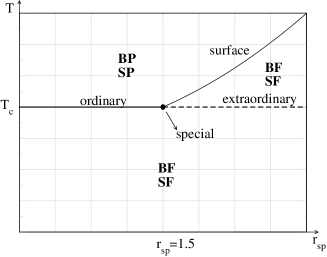
Figure 1: Schematic phase diagram for the semi-infinite Ising model with bulk coupling $J_{b}$ and surface coupling ratio $J_{s}/J_{b}$. $T_{b}$ is the bulk transition temperature and the ferromagnetic bulk is denoted by FB while the paramagnetic is denoted by PB. The surface phases are labeled FS for a ferromagnet and PS for a paramagnet.

For a non-perfect surface, we introduce a defect line with coupling strength $J_{l}$ onto the surface. Generally speaking, the impact of imperfection on a surface is two fold. Take a surface with random bond disorder as an example. The randomness may reduce the surface transition temperature, and alter the global phase diagram of a semi-infinite system. For example, the special transition point of the Ising model with a amorphous surface is located at $r_{sp}=1.70(1)$ M. Pleimling and W. Selke (1998a), noticeably larger than that of the Ising model with a perfect surface $r_{sp}=1.5004$. Another effect of the randomness is that it may change the universality class of the surface. The relevance or irrelevance of random imperfections on the pure surface can be assessed by the Harris-type criterion H.W. Diehl and A. Nüsser (1990). The extended-Harris criterion states that for a surface with random bond disorder, the disorder is relevant for $\alpha_{11}>0$ but irrelevant for $\alpha_{11}<0$. Based on this criterion, the random surface coupling of the Ising model is irrelevant at the ordinary transition since $\alpha_{11}<0$. In this case, it was rigorously proved $\beta_{1}^{dis}=\beta_{1}^{ord}$ by Diehl based on the Griffiths-Kelly-Sherman inequality, where $\beta_{1}^{dis}$ is the critical exponent at the ordinary transition on a random bond surfaceH.W. Diehl (1998). The situation is less clear at the special transition, for $\alpha_{11}$ is very close to $0$. Recent simulations suggest that $\alpha_{11}<0$ and hence the disorder is irrelevantY. Deng, H.W.J. Blöte, and M.P. Nightingale (2005). The irrelevance at the special transition has also been reported in Ref. M. Pleimling and W. Selke (1998a). At the surface transition, the surface is equivalent to the $2d$ Ising model. The disorder only leads to logarithm correction (see H.J. Luo, L. Schülke, B. Zheng (2001) and reference therein). In the case of defect line, the defect doesn’t shift the transition temperatures of the surface transition, and therefore, the special transition point $r_{sp}$ at which the surface transition line and ordinary transition line meet remains to be unchanged M.E. Fisher and A.E. Ferdinand (1967). We only consider the robustness of the ordinary, special and surface transition in the presence of line defect.

II.2 Dynamic scaling analysis

Table 1: The bulk critical temperature and critical exponents of the $3d$ Ising model.

$T_{c}$	$\nu_{3d}$	$z_{3d}$
$4.5115248(6)$ Y. Deng and H.W.J. Blöte (2003)	$0.6298(5)$ A.M. Ferrenberg and D.P. Landau (1991)	$2.042(6)$ A. Jaster, J. Mainville, L. Schülke, and B. Zheng (1999)

For a dynamic system, which is initially in a high-temperature state, suddenly quenched to the critical temperature, and then released to the dynamic evolution of model A, one expects that there exist universal scaling behaviors already in the macroscopic short-time regime H.K. Janssen, B. Schaub and B. Schmittmann (1989). This has been shown both theoretically and numerically in a variety of statistical systems H.K. Janssen, B. Schaub and B. Schmittmann (1989); Huse (1989); Zheng (1998); B. Zheng, M. Schulz, and S. Trimper (1999); C. Godréche and J.M. Luck (2002); P. Calabrese and A. Gambassi (2005); B. Zheng, F. Ren, and H. Ren (2003); J.Q. Yin, B. Zheng, and S. Trimper (2005), and it explains also the spin glass dynamics. Furthermore, the short-time dynamic scaling behavior has been extended to the dynamic relaxation with an ordered initial state or arbitrary initial state, based on numerical simulations Zheng (1998); B. Zheng, F. Ren, and H. Ren (2003); J.Q. Yin, B. Zheng, and S. Trimper (2005); B. Zheng (1996); A. Jaster, J. Mainville, L. Schülke, and B. Zheng (1999). Recent renormalization group calculations also support the short-time dynamic scaling form for the ordered initial state A.A. Fedorenko and S. Trimper (2006).

On the other hand, Ritschel and Czerner have generalized the short-time critical dynamics in a homogenous system to that in an inhomogeneous one, i.e., the systems with a free surface, and derived the scaling behavior of the magnetization close to the surface for the dynamic relaxation with a high-temperature initial state Ritschel and Czerner (1995). Recent development can be found in Refs. M. Pleimling and F. Iglói (2004, 2005). In this paper, we alternatively focus on the dynamic relaxation with the ordered initial state, and with a non-perfect surface. As pointed out in the literatures Zheng (1998); B. Zheng, F. Ren, and H. Ren (2003), the fluctuation is less severe in this case. It helps to obtain a more accurate estimate of the critical exponents at surface. From theoretical point of view, it is also interesting to study the dynamic relaxation with the ordered or even arbitrary initial state.

Similar to the scaling analysis in bulk H.K. Janssen, B. Schaub and B. Schmittmann (1989); Zheng (1998); A. Jaster, J. Mainville, L. Schülke, and B. Zheng (1999); A.A. Fedorenko and S. Trimper (2006), we phenomenologically assume that, for dynamic relaxation with ordered initial state, the surface magnetization decays by a power law,

$$<m_{1}(t)>\sim t^{-\beta_{1}/\nu_{s}z_{s}},$$ (2)

after a microscopic time scale $t_{mic}$. Here $<\cdot>$ represents the statistical average, $\beta_{1}$ is the static exponent of the surface magnetization, $\nu_{s}$ is the static exponent of the spatial correlation length, and $z_{s}$ is the dynamic exponent. This assumption can be understood by noting that, for nonequilibrium preparation with ordered initial state $m_{0}=1$, the dynamic relaxation is governed by critical thermal fluctuation with scaling dimension $x_{1}=\beta_{1}/\nu_{s}$. For the ordinary and special transitions where the criticality of surface originates from the divergence of the correlation length in bulk, there are no genuine new surface dynamic exponent $z_{s}$ and static exponent $\nu_{s}$. $\nu_{s}$ and $z_{s}$ are just the same as those in the bulk, i.e. $\nu_{s}=\nu_{3d}$ and $z_{s}=z_{3d}$, while $\beta_{1}$ is neither that of the $2d$ Ising model nor that of the $3d$ Ising model S. Dietrich and H.W. Diehl (1983). For the surface transition where the critical fluctuation of surface is of the universality class of the $2d$ Ising model, it is generally believed that all static and dynamic exponents are the same as those of the $2d$ Ising model K. Binder (1987); H.W. Diehl (1987). i.e. $\beta_{1}=\beta_{2d}=1/8$, $\nu_{s}=\nu_{2d}=1$ and $z_{s}=z_{2d}\approx 2.16(2)$ Zheng (1998).

Table 2: Summary of the surface critical exponents at the ordinary and special transition in the $3d$ Ising model, as obtained by different techniques. MF: mean-field, MC: Monte Carlo simulations, FT: field-theoretical methods, CI: conformal invariance. The data marked with $*$ are calculated by using scaling law $2\beta_{1}+\gamma_{11}=(d-1)\nu_{s}$.

	MF K. Binder (1987)	MC D.P. Landau and K. Binder (1990)	MC C. Ruge and F. Wagner (1995)	MC M. Pleimling and W. Selke (1998b)	MC Y. Deng, H.W.J. Blöte, and M.P. Nightingale (2005)	MC C. Ruge, A. Dunkelmann, F. Wagner and J. Wulf (1993)	MC+CI Y. Deng and H.W.J. Blöte (2003)	FT H.W. Diehl and M. Shpot (1998)	this work
$\beta_{1}^{ord}$	$1$	$0.78(2)$	$0.807(4)$	$0.80(1)$	$0.796(1)$	$-$	$0.798(5)$	$0.796$	$0.795(6)$
$\beta_{1}^{sp}$	$1/2$	$0.18(2)$	$0.238(2)$	$-$	$0.229(1)$	$0.237(5)$	$-$	$0.263$	$0.220(3)$
$\gamma_{11}^{sp}$	$1/2$	$0.96(9)$	$0.788(1)$	$-$	$0.802(3)^{*}$	$0.785(11)^{*}$	$-$	$0.734$	$0.823(4)$

Another important observable is the second moment of the surface magnetization, or the so-called time-dependent surface susceptibility, defined as

$$\chi_{11}=L^{2}[<m_{1}^{2}>-<m_{1}>^{2}].$$ (3)

Simple finite-size scaling analysis Zheng (1998) reveals that

$$\chi_{11}(t)\sim t^{\gamma_{11}/\nu_{s}z_{s}}.$$ (4)

Here the exponent $\gamma_{11}/\nu_{s}$ is related to $\beta_{1}/\nu_{s}$ by $\gamma_{11}/\nu_{s}=d-1-2\beta_{1}/\nu_{s}$, with $d=3$ being the spatial dimension of bulk. This is nothing but the scaling law in equilibrium between the exponent of the surface susceptibility and the exponent of the surface magnetization. One can also understand the scaling behavior in Eq. (4) in an intuitive way. In equilibrium, $\chi_{11}$ behaves as $\chi_{11}\sim L^{\gamma_{11}/\nu_{s}}$ with $L$ being the lattice size. In the dynamic evolution, $\chi_{11}(t)$ should be related to the non-equilibrium spatial correlation length $\xi(t)$ with $\chi_{11}(t)\sim\xi(t)^{\gamma_{11}/\nu_{s}}$, since the finite size effect is negligible. Then the growth law $\xi(t)\sim t^{1/z_{s}}$ of the non-equilibrium spatial correlation length immediately leads to Eq. (4).

Alternatively, one can also construct the appropriate time-dependent cumulant $U(t)=<m_{1}^{2}>/<m_{1}>^{2}-1$. Obviously, $U(t)\sim t^{(\gamma_{11}+2\beta_{1})/\nu_{s}z_{s}}$. From the scaling law $\gamma_{11}/\nu_{s}=d-1-2\beta_{1}/\nu_{s}$, one derives $(\gamma_{11}+2\beta_{1})/\nu_{s}=d-1$. The scaling behavior of $U(t)$ then reduces to the standard form Zheng (1998); A. Jaster, J. Mainville, L. Schülke, and B. Zheng (1999),

$$U(t)\sim t^{(d-1)/z_{s}},$$ (5)

with $d-1$ being the spatial dimension of the surface.

In other words, from Eqs. (2) and (4), or from Eqs. (2) and (5), we obtain independent measurements of two critical exponents, e.g., $\beta_{1}/\nu_{s}$ and $z_{s}$. Alternatively, if we take $\nu_{s}$ and $z_{s}$ as input, we have two independent estimates of the static exponent $\beta_{1}$ of the surface magnetization. This may testify the consistency of our dynamic scaling analysis.

All foregoing equations involve the bulk exponents $\nu_{s}$ and $z_{s}$. Therefor an accurate estimate of the surface critical exponents $\beta_{1}$ needs precise values of $\nu_{3d}$ and $z_{3d}$, as well as $z_{2d}$. Since the $3d$ bulk Ising model has been extensively studied with various methods, many accurate results of the critical exponents and transition temperature are available. We concentrate our attention to the surface exponents and take the bulk exponents as input. The results of the bulk exponents of the $3d$ Ising model are summarized in Table 1. The criteria to choose those values are their relative accuracy, as well as the methods used to extract these exponents.

II.3 Simulations

In this paper, with Monte Carlo simulations we study the dynamic relaxation of the $3d$ Ising model on a perfect and non-perfect surface at the transition temperature, quenched from a completely ordered initial state. The standard Metropolis algorithm is adopted in the simulations. In order to investigate the surface critical behavior, we apply the periodic boundary condition in the $xy$ plane and open boundary condition in the z direction to the $L\times L\times L$ cubic lattice.

The main results are obtained with the lattice size $L=128$ and $L=80$, and additional simulations with other lattice sizes are also performed to study the finite-size effect. For a perfect surface, the surface magnetization is defined as

$$m_{1}=\frac{1}{2L^{2}}\sum_{xy}^{L}(\sigma_{xy1}+\sigma_{xyL}),$$ (6)

and its critical exponent is denoted by $\beta_{1}$. For a non-perfect surface, the defect line is placed at surface position $x=L/2$ and the line magnetization is defined as

$$m_{2}=\frac{1}{2L}\sum_{xy}^{L}(\sigma_{\frac{L}{2}y1}+\sigma_{\frac{L}{2}yL}),$$ (7)

and its critical exponent is denoted by $\beta_{2}$. The spin $\sigma_{xyz}$ denotes the spin sitting at site $(x,y,z)$. We measure the surface and line magnetization during the nonequilibrium relaxation. We average from $5000$ to $20000$ runs with different random numbers to achieve a good statistics. Error bars are estimated by dividing the total samples into two subgroups, and by measuring the exponents at different time intervals. Most of the simulations are carried out on the Dawning 4000A supercomputer. The total CPU time is about $3$ node-year.

III Short-time dynamics on a perfect surface

In this section we study the nonequilibrium critical dynamics on a perfect surface, i.e. $J_{l}=J_{s}$. To investigate the critical behavior on the surface, it is important to know the special transition point $r_{sp}$. For a perfect surface of the $3d$ Ising model with ferromagnetic interactions, there exist rather accurate estimates of $r_{sp}$ in equilibrium, e.g., $r_{sp}=1.5004(20)$ in Ref. C. Ruge, S. Dunkelmann, and F. Wagner (1992). We adopt this value as the special transition point. As illustrated later, the special transition point $r_{sp}$ can also be estimated from the scaling plot of a dynamic crossover scaling relation.

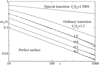
Figure 2: Dynamic relaxation of the surface magnetization is displayed with solid lines on a double-log scale, at the ordinary transition with various $J_{s}/J_{b}$, and at the special transition $J_{s}/J_{b}=r_{sp}=1.5004$. The temperature is set to the bulk critical temperature $T_{c}$, and the lattice size is $L=80$. Open circle are the data for $J_{s}/J_{b}=1.0$ and $L=40$. Well away from the special transition, the slope of the curves is independent of $J_{s}/J_{b}$.

Figure 3: Dynamic relaxation of the surface susceptibility and cumulant at the special transition is plotted on a double-log scale. The lattice size is $L=128$ and $T=T_{c}$.

For the ordinary phase transition, the dynamic relaxation of the surface magnetization with different $J_{s}/J_{b}$ are shown in Fig. 2. The curves of $J_{s}/J_{b}=1.0$ with $L=40$ and $L=80$ overlap up to $t\geq 300$MCS(Monte Carlo sweep per site). It confirms that the finite-size effect is negligibly small for $L=80$ up to at least $t=1000$MCS, since the correlating time of a finite system increases by $t_{L}\sim L^{z}$. In Fig. 2, a power-law behavior is observed for all $J_{s}/J_{b}$. The microscopic time scale $t_{mic}$, after which the short-time universal scaling behavior emerges, in other words, after which the correction to scaling is negligible, gradually increases as the surface coupling is being enhanced. For $J_{s}/J_{b}=0.2$, $t_{mic}\sim 10$MCS, while for $J_{s}/J_{b}=1.2$, $t_{mic}\sim 100$MCS.

A direct observation in Fig. 2 is that the curves for $J_{s}/J_{b}<r_{sp}$ are parallel to each other. By fitting these curves to Eq. (2), we obtain $\beta_{1}^{ord}=0.790(7)$, $0.792(6)$, $0.795(6)$, $0.786(6)$ and $0.755(12)$ for $J_{s}/J_{b}=0.2$, $0.5$, $0.8$, $1.0$ and $1.2$ respectively. The values of $\beta_{1}^{ord}$ at $J_{s}/J_{b}=0.2$, $J_{s}/J_{b}=0.5$ and $J_{s}/J_{b}=0.8$ are well consistent with each other within error. It indicates that the ordinary transition is universal over a wide range in the $J_{s}/J_{b}$ space. Deviation occurs for $J_{s}/J_{b}>1.0$ and manifests itself as the effect of the crossover to the special transition. This is in agreement with the observation in Ref. D.P. Landau and K. Binder (1990). From our analysis, $\beta_{1}^{ord}=0.795(6)$ is a good estimate for the ordinary transition. In Table 2, we have compile all the existing results which were obtained with simulations and analytical calculations in equilibrium, and our measurements from the non-equilibrium dynamic relaxation. A reasonable agreement in $\beta_{1}^{ord}$ can be observed. Part of the statistical error in our dynamic measurements is from the input of the bulk exponents $\nu_{s}$ and $z_{s}$.

With $m_{1}(t)$ at hand, one may proceed to investigate the time-dependent susceptibility, $\chi_{11}(t)$. In the case of the ordinary transition of the $3d$ Ising model, however, $\gamma_{11}$ is negative. Therefore the $\chi_{11}$ is suppressed during the time relaxation according to Eq. (4) and fluctuating around $0$ if nonequilirium preparation is an ordered initial state $\chi_{11}(0)=0$. The power-law behavior in Eq. (4) could not be observed. Nevertheless, at the special transition, where $\gamma_{11}$ is positive, the situation is different. The power-law behavior of the surface susceptibility and cumulant shows up.

In Fig. 2 and 3, the surface magnetization, surface susceptibility and appropriate cumulant are displayed at the special transition $J_{s}/J_{b}=r_{sp}$. A power-law behavior is observed for all three observables. From the slope of the curve of the surface magnetization, we measure $\beta_{1}^{sp}/\nu_{s}z_{s}=0.171(2)$, and then obtain $\beta_{1}^{sp}=0.220(3)$ with $\nu_{s}$ and $z_{s}$ in Table 1 as input. From the curve of the surface susceptibility, we measure $\gamma_{11}^{sp}/\nu_{s}z_{s}=0.640(3)$, and then calculate $\gamma_{11}^{sp}=0.823(4)$. From the scaling law $\gamma_{11}/\nu_{s}=d-1-2\beta_{1}/\nu_{s}$, one derives $\beta_{1}^{sp}=0.218(2)$, which is in good agreement with $\beta_{1}^{sp}=0.220(3)$ estimated from the surface magnetization. The scaling behaviors in Eqs. (2) and (4) indeed hold.

The remarkable feature of the cumulant on the surface is that its scaling behavior in Eq. (5) does not involve the exponent $\beta_{1}$ of the surface magnetization. From the curve in Fig. 3, we obtain $(d-1)/z_{s}=0.996(11)$, then calculate the bulk dynamic critical exponent $z_{s}=2.01(2)$. This value of $z_{s}$ is very close to $z_{3d}=2.04(1)$ measured in numerical simulations in the bulk in Table 1, and it confirms that the dynamic exponent on the surface is the same as that in the bulk.

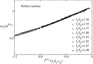
Figure 4: The scaling plot of $m_{1}(t)$ according to Eq. (9) around the special transition $J_{s}/J_{b}=r_{sp}=1.5004$. The time window in this plot is within $[10,1000]$. The lattice size is $L=80$ and $T=T_{c}$.

In order to describe the dynamic behavior of the surface magnetization around $r_{sp}$, we need to introduce a crossover scaling relation. To understand the scaling relation in non-equilibrium states, we first recall the crossover scaling relation in equilibrium. In equilibrium, $m_{1}(\tau)$ near the special transition is described by a crossover scaling relation

$$m_{1}(\tau)\tau^{-\beta_{1}^{sp}}=M_{eq}(\tau^{-\phi}(J_{s}/J_{b}-r_{sp})),$$ (8)

where $\tau=1-T/T_{c}$ is the reduced temperature, and $\phi$ is the crossover exponent. From the crossover scaling relation of $m_{1}(\tau)$ , one can determine the special transition point $r_{sp}$ as well as $\beta_{1}^{sp}$ and $\phi$ D.P. Landau and K. Binder (1990). Nevertheless, up to now it has not been studied whether there also exists a corresponding crossover scaling relation in non-equilibrium states. Here we will verify that such a dynamic crossover scaling form indeed exists. For simplicity, we consider the case when $J_{s}/J_{b}$ approaches the special transition from $r_{sp}^{-}$ and the system is at the bulk critical temperature. Now the non-equilibrium spatial correlation length $\xi(t)\sim t^{1/z}$ takes the place of the equilibrium spatial correlation length $\tau^{-\nu}$. By substituting $t^{-1/\nu_{s}z_{s}}$ for $\tau$ into Eq. (8), we obtain

$$m_{1}(t)t^{\beta_{1}^{sp}/\nu_{s}z_{s}}=M_{neq}(t^{\phi/\nu_{s}z_{s}}(J_{s}/J_{b}-r_{sp})).$$ (9)

We have performed non-equilibrium simulations at $J_{s}/J_{b}=1.30$, $1.35$, $1.37$, $1.40$, $1.43$, $1.45$, $1.47$, $1.49$, and made a scaling plot according to Eq. (9). This is demonstrated in Fig. 4. All curves of different $J_{s}/J_{b}$ collapse into a single master curve, and it indicates that Eq. (9) does describe the crossover behavior during the dynamic relaxation. The scaling plot in Fig. 4 yields the exponents $\phi=0.52$ and $\beta_{1}^{sp}=0.220$, as well as the special transition point $r_{sp}=1.50$. The crossover exponent $\phi$ is very close to the mean-field value $0.5$ D.P. Landau and K. Binder (1990), and $\beta_{1}^{sp}$ and $r_{sp}$ are in agreement with the existing results from simulations in equilibrium in Table 2 and in Ref. C. Ruge, S. Dunkelmann, and F. Wagner (1992). Although the precision of $r_{sp}$ and critical exponents obtained here are not very high, it is still theoretically interesting. The dynamic crossover scaling form in Eq. (9) should be general, and hold in various statistical systems.

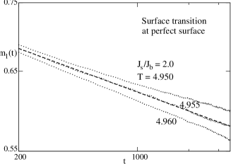
Figure 5: Determination of the surface transition temperature $T_{s}$ for $J_{s}/J_{b}=2.0$. The dashed line is a power-law fit to the curve of $T=4.955$. The lattice size is $L=80$.

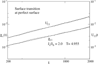
Figure 6: Dynamic relaxation of the surface susceptibility and cumulant at the surface transition $J_{s}/J_{b}=2.0$ plotted on double-log scale. The lattice size is $L=80$ and $T_{s}=4.955$. The dashed lines are power-law fits to the curves.

To carry out the simulation at the surface transition, we fix $J_{s}/J_{b}$ at $2.0$, well above $r_{sp}$. At the surface transition, where the critical fluctuation is essentially two dimensional, $\nu_{s}$ and $z_{s}$ in Eq. (2) become $\nu_{2d}$ and $z_{2d}$. Around the transition temperature, the surface magnetization obeys a dynamic scaling form $<m_{1}(t)>\sim t^{-\beta_{1}/\nu_{s}z_{s}}F(t^{1/\nu_{s}z_{s}}\tau)$ Zheng (1998). To determine the surface transition temperature $T_{s}$, one may search for a best-fitting power-law curve to the surface magnetization. Then the corresponding temperature is identified as the transition temperature $T_{s}$. We perform the simulations with three temperatures around the transition temperature $T_{s}$, and measure the surface magnetization. The results are displayed in Fig. 5. Interpolating the surface magnetization to other temperatures around these three temperatures, one finds the best power-law behavior of the surface magnetization at $T_{s}=4.955$. The corresponding slope of the curve gives $\beta_{1}/z_{s}=0.0570(10)$ at $T_{s}=4.955$, and it is in agreement with the value in the $2d$ Ising model Zheng (1998). Therefore we take $T_{s}=4.955$ as the surface transition temperature, which is consistent with $T_{s}=4.9575(75)$ obtained with Monte Carlo simulations in equilibrium M. Pleimling and W. Selke (1999).

The time-dependent cumulant $U$ and susceptibility $\chi_{11}$ at the surface transition are measured, and displayed in Fig. 6. The slope of cumulant is $0.916(15)$, in a good agreement with $2/z_{2d}=0.926(9)$ of the $2d$ Ising model Zheng (1998). Consistence is also observed for the susceptibility where the slope is $0.824(10)$, in comparison with $\gamma_{2d}/z_{2d}=0.810(8)$ in the $2d$ Ising model. We thus confirm that the surface transition belongs to the universality class of the $2d$ Ising model. Meanwhile, $T_{s}=4.955$ is a good estimate of the surface transition temperature.

IV Short-time dynamics on a non-perfect surface

In this section we investigate the nonequilibrium critical dynamics on a non-perfect surface, i.e. $J_{l}\neq J_{s}$. The static and dynamic properties of a non-perfect surface are important and interesting, because real surfaces are often rough, due to the impurity or limitation of experimental conditions M. Pleimling (2004). Furthermore, the advance in nano-science allows experimentalists to create other structures on top of films artificially. We study the line defect on a surface, and the procedure can be generalized to other extended defects.

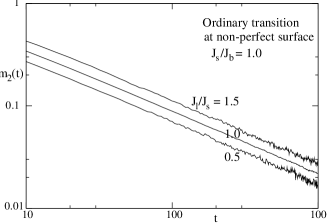
Figure 7: Dynamic relaxation of the line magnetization at the ordinary transition on a non-perfect surface with various $J_{l}$ is plotted on a double-log scale. The slope of the curves is independent of $J_{l}$.

We first consider the dynamic behavior of $m_{2}$ at the ordinary transition. For convenience, we fix $J_{s}/J_{b}=1.0$. The profiles of $m_{2}(t)$ with $J_{l}=0.5J_{s}$, $J_{l}=1.0J_{s}$ and $J_{l}=1.5J_{s}$ are depicted in Fig. 7. All lines look parallel to each other, and it indicates that they may belong to a same universality class. By fitting these curves to the power law in Eq. (2), we estimate $\beta_{2}^{ord}=0.792(18)$, $0.786(6)$ and $0.797(33)$ with $J_{l}=1.5J_{s}$, $J_{l}=1.0J_{s}$ and $J_{l}=0.5J_{s}$ respectively. These values are consistent with each other and with $\beta_{1}^{ord}$ on the perfect surface reported in the previous section. It confirms that the defect in the ordinary transition is irrelevant, in term of the renormalization group argument. This conclusion echoes that in Ref. M. Pleimling and W. Selke (1998a), where the impact of random bonds on the surface is investigated in equilibrium. According to the generalized Harris criterion H.W. Diehl and A. Nüsser (1990), defects with random bonds or diluted bonds on a surface are irrelevant. The short-time dynamic approach shows its merits in identifying the universal behavior of the surface magnetization M. Pleimling and W. Selke (1998a, b); M. Pleimling and W. Selke (1999, 2000). Here we note that the line magnetization is one-dimensional, and therefore somewhat more fluctuating than the surface magnetization.

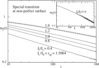
Figure 8: Dynamic relaxation of the line magnetization at the special transition $J_{s}/J_{b}=r_{sp}=1.5004$ on a non-perfect surface with various $J_{l}$ is plotted on a double-log scale. The open circles are a fit to Eq. (10) with a correction to scaling. The inset displays the line magnetization at $J_{l}=1.6J_{s}$ but with a longer simulation time. The lattice size is $L=128$ and $T=T_{c}$. The slope of the curves is dependent on $J_{l}$ even after taking the correction to scaling into account.

Figure 9: Dynamic relaxation of the line magnetization with various $J_{l}$ at the surface transition is plotted on a double-log scale. The lattice size is $L=80$ and $T=T_{s}$. The slope of the curves is dependent on $J_{l}$, and given in Table 3.

Now we turn to the special transition. We perform simulations with various $J_{l}$ at the special transition, and the line magnetization is presented in Fig. 8. From the slopes of the curves, one measures the exponent $\beta_{2}^{sp}/\nu_{s}z_{s}$, and then calculates $\beta_{2}^{sp}=0.260(4)$, $0.230(3)$, $0.219(5)$, $0.204(6)$ and $0.162(3)$ for $J_{l}=0.4J_{s}$, $J_{l}=0.8J_{s}$, $J_{l}=1.0J_{s}$, $J_{l}=1.2J_{s}$ and $J_{l}=1.6J_{s}$ respectively, with $\nu_{s}$ and $z_{s}$ taken as input from Table 1. Obviously $\beta_{2}^{sp}$ changes continuously with $J_{l}$.

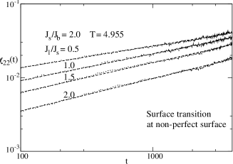
Figure 10: Dynamic relaxation of the line susceptibility with various $J_{l}$ at the surface transition plotted on a double-log scale. The dashed lines are power-law fits. The slope of the curves is dependent on $J_{l}$, and given in Table 3.

Since there exists certain deviation from a power law in shorter times for the curves with a larger ratio $J_{l}/J_{s}$ in Fig. 8, one may wonder whether the small variation in $\beta_{2}^{sp}$ may stem from the correction to scaling induced by the defect line. Therefore, a careful analysis of the correction to scaling is necessary in this case. Assuming a power-law correction to scaling, $m_{2}(t)$ should evolve according to

$$m_{2}(t)=at^{-\beta_{2}^{sp}/\nu_{s}z_{s}}(1-bt^{-c}).$$ (10)

As shown in Fig. 8, such an ansatz fits the numerical data very well, and yields $\beta_{2}^{sp}=0.258(1)$, $0.235(7)$, $0.228(3)$, $0.214(6)$ and $0.171(3)$ for $J_{l}=0.4J_{s}$, $J_{l}=0.8J_{s}$, $J_{l}=1.0J_{s}$, $J_{l}=1.2J_{s}$ and $J_{l}=1.6J_{s}$ respectively. For $J_{l}=1.6J_{s}$, we extend our simulations up to a maximum time $t=10000$MCS to gain more confidence on our results. Still $\beta_{2}^{sp}$ varies continuously with $J_{l}$, and the strong universality is violated. This is different from the case on a random surface, where the generalized Harris criterion states that the enhancement of the short-range randomness on the surface is irrelevant at the surface transition in the $3d$ Ising model H.W. Diehl and A. Nüsser (1990). Our result is, however, not surprising, for the defect line is not a short-range randomness M. Pleimling (2004), but an extended one. As the short-range random surface is close to being relevant M. Pleimling (2004), it is not surprising that the defect line modifies the surface universality class. This can also be understood. The reduction of the coupling in the defect line is somewhat like turning the local surface from the special transition to the ordinary one, and therefore gives rise to a large value of the critical exponent $\beta_{2}^{sp}$.

Table 3: Comparison between the numerical simulations of surface transition with a non-perfect surface and the theory of the two-dimensional Ising model with a defect line. $\nu_{s}=\nu_{2d}=1$ and $z_{s}=z_{2d}=2.16(2)$ have been taken as input Zheng (1998).

	line magnetization		susceptibility		cumulant
exponent	$\beta_{2}/z_{s}$		$(1-2\beta_{2})/z_{s}$		$1/z_{s}$
	Simulation	Theory	Simulation	Theory	Simulation	Theory
$J_{l}=0.5J_{s}$	$0.0923(36)$	$0.0936(9)$	$0.282(4)$	$0.276(3)$	$0.462(2)$	$0.463(4)$
$J_{l}=1.0J_{s}$	$0.0570(10)$	$0.0579(5)$	$0.356(5)$	$0.347(3)$	$0.475(2)$	$0.463(4)$
$J_{l}=1.5J_{s}$	$0.0301(24)$	$0.0307(3)$	$0.405(4)$	$0.402(4)$	$0.468(2)$	$0.463(4)$
$J_{l}=2.0J_{s}$	$0.0149(12)$	$0.0145(1)$	$0.428(9)$	$0.434(4)$	$0.459(9)$	$0.463(4)$

To investigate the impact of the line defect at the surface transition, we fix $J_{s}/J_{b}=2.0$. We measure the time evolution of the line magnetization at its transition temperature $T_{s}=4.955$ with $J_{l}=0.5J_{s}$, $J_{l}=1.0J_{s}$, $J_{l}=1.5J_{s}$ and $J_{l}=2.0J_{s}$. In Fig. 9, one observes that after a microscopic time $t_{mic}\sim 100$MCS, the power-law behavior emerges. However, the exponent $\beta_{2}$ is $J_{l}$-dependent, and the strong universality is violated. This is similar to the case in Ref. M. Pleimling and W. Selke (1999, 2000), where a non-universal behavior of the edge and corner magnetization has been found at the surface transition.

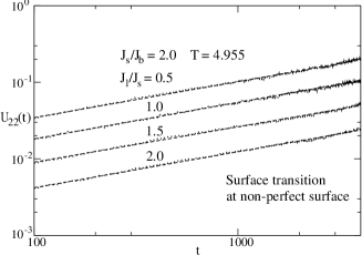
Figure 11: Dynamic relaxation of the cumulant with various $J_{l}$ at the surface transition plotted on a double-log scale. The dashed lines are power-law fits. The slope of the curves is independent of $J_{l}$, and given in Table 3.

Since the surface transition is essentially two-dimensional, one may relate this non-perfect surface to the $2d$ Ising model with a defect line without the presence of bulk. The violation of the strong universality of the $2d$ Ising model with a line or a ladder defect is rigorously proved by Bariev R. Z. Bariev (1979). For the line defect, exact calculations show that

$$\beta_{2}=\frac{2}{\pi^{2}}\arctan^{2}(\kappa_{l}),$$ (11)

with

$$\kappa_{l}=\exp(-2(J_{l}-J)/k_{B}T_{c}).$$ (12)

The critical exponent $\beta_{2}$ reduces monotonically, when the defect coupling $J_{l}$ is enhanced. We measure the exponent $\beta_{2}$ and compare it with the exact values obtained from Eqs. (11) and (12). The results are summarized in Table 3. One finds a good agreement between simulations and exact results. A similar behavior of the edge magnetization, which can be viewed as a line defect at the surface transition, is also observed in Ref. M. Pleimling and W. Selke (1999). Our results support that at the surface transition, the critical exponent $\beta_{2}$ will change in the presence of a small perturbation.

Finally, the susceptibility $\chi_{22}(t)$ and cumulant $U_{22}(t)$ of the line magnetization, which are similarly defined as those of the surface magnetization, are also measured. The results are plotted in Fig. 10 and 11. Simple scaling analysis shows that $\chi_{22}(t)\sim t^{(d-2-2\beta_{2}/\nu_{s})/z_{s}}$ and $U_{22}(t)\sim t^{(d-2)/z_{s}}$. The estimated exponents are also compiled in Table 3, and a good consistency with the theory can be spotted.

V Conclusion

With Monte Carlo simulations, we have studied the dynamic relaxation on a perfect and non-perfect surface in the $3d$ Ising model, starting from an ordered initial state. On the perfect surface, the dynamic behavior of the surface magnetization, susceptibility and appropriate cumulant is carefully analyzed at the ordinary, special and surface transition. The universal dynamic scaling behavior is revealed, and the static exponent $\beta_{1}$ of the surface magnetization, the static exponent $\gamma_{11}$ of the surface susceptibility and the dynamic exponent $z_{s}$ are estimated. All the results for $\beta_{1}$ are compiled in Table 2. Since the exponents $\nu_{s}$ and $z_{s}$ can be identified as those at bulk, it is convenient to study different phase transitions from the non-equilibrium dynamic relaxation. Especially, the dynamic crossover scaling form in Eq. (9) is interesting. Because of the existence of new scaling variable $J_{s}/J_{b}$, the nonequilibrium relaxation of magnetization at the critical temperature may not obey a power law, which is quite different from the general systems investigated so far where a power law behavior was always expected. This unusual nonequilibrium behavior is a consequence of the presence of geometric surface.

On the non-perfect surface, i.e., with a defect line in the surface, the universality class of the ordinary transition remains the same as that at the perfect surface. On the other hand, for the special and surface transitions, the critical exponent $\beta_{2}$ of the line magnetization varies with the coupling $J_{l}$ strength of the defect line. The susceptibility and appropriate cumulant of the line magnetization also exhibit the dynamic scaling behavior and yield the static exponent $\gamma_{22}$ and the dynamic exponent $z_{s}$. The short-time dynamic approach is efficient in understanding the surface critical phenomena.

Acknowledgements: This work was supported in part by NNSF (China) under Grant No. 10325520. The authors would like to thank M. Pleimling for helpful discussions. One of the authors (SZL) would like to thank L. Y. Wang for critical reading this manuscript. The computations are partially carried out in Shanghai Supercomputer Center.

References

- M.A. Torija, A.P. Li, X.C. Guan, E.W. Plummer, and J. Shen (2005) M.A. Torija, A.P. Li, X.C. Guan, E.W. Plummer, and J. Shen, Phys. Rev. Lett. 95, 257203 (2005).
- K. Binder (1987) K. Binder, in Phase Transition and Critical Phenomena (Academic Press, London, 1987), vol. 8, p.1, and references therein.
- H.W. Diehl (1987) H.W. Diehl, in Phase Transition and Critical Phenomena (Academic Press, London, 1987), vol. 10, p.76, and references therein.
- H.W. Diehl (1997) H.W. Diehl, Int. J. Mod. Phys. B11, 3503 (1997).
- M. Pleimling (2004) M. Pleimling, J. Phys. A37, R79 (2004).
- K. Binder and P.C. Hohenberg (1972) K. Binder and P.C. Hohenberg, Phys. Rev. B6, 3461 (1972).
- K. Binder and D.P. Landau (1984) K. Binder and D.P. Landau, Phys. Rev. Lett. 52, 318 (1984).
- D.P. Landau and K. Binder (1990) D.P. Landau and K. Binder, Phys. Rev. B41, 4633 (1990).
- C. Ruge and F. Wagner (1995) C. Ruge and F. Wagner, Phys. Rev. B52, 4209 (1995).
- Y. Deng, H.W.J. Blöte, and M.P. Nightingale (2005) Y. Deng, H.W.J. Blöte, and M.P. Nightingale, Phys. Rev. E72, 016128 (2005).
- S. Dietrich and H.W. Diehl (1983) S. Dietrich and H.W. Diehl, Z. Phys. B51, 343 (1983).
- M. Kikuchi and Y. Okabe (1985) M. Kikuchi and Y. Okabe, Phys. Rev. Lett. 55, 1220 (1985).
- H.W. Diehl (1994) H.W. Diehl, Phys. Rev. B49, 2846 (1994).
- H.K. Janssen, B. Schaub and B. Schmittmann (1989) H.K. Janssen, B. Schaub and B. Schmittmann, Z. Phys. B 73, 539 (1989).
- Huse (1989) D. Huse, Phys. Rev. B 40, 304 (1989).
- Zheng (1998) B. Zheng, Int. J. Mod. Phys. B12, 1419 (1998), review article.
- B. Zheng, M. Schulz, and S. Trimper (1999) B. Zheng, M. Schulz, and S. Trimper, Phys. Rev. Lett. 82, 1891 (1999).
- C. Godréche and J.M. Luck (2002) C. Godréche and J.M. Luck, J. Phys.:Condens. Matter 14, 1589 (2002).
- P. Calabrese and A. Gambassi (2005) P. Calabrese and A. Gambassi, J. Phys. A38, R133 (2005).
- Z.B. Li, L. Schülke, and B. Zheng (1995) Z.B. Li, L. Schülke, and B. Zheng, Phys. Rev. Lett. 74, 3396 (1995).
- H.J. Luo, L. Schülke, and B. Zheng (1998) H.J. Luo, L. Schülke, and B. Zheng, Phys. Rev. Lett. 81, 180 (1998).
- L. Schülke and B. Zheng (2000) L. Schülke and B. Zheng, Phys. Rev. E62, 7482 (2000).
- B. Zheng, F. Ren, and H. Ren (2003) B. Zheng, F. Ren, and H. Ren, Phys. Rev. E68, 046120 (2003).
- J.Q. Yin, B. Zheng, and S. Trimper (2004) J.Q. Yin, B. Zheng, and S. Trimper, Phys. Rev. E70, 056134 (2004).
- J.Q. Yin, B. Zheng, and S. Trimper (2005) J.Q. Yin, B. Zheng, and S. Trimper, Phys. Rev. E72, 036122 (2005).
- A.A. Fedorenko and S. Trimper (2006) A.A. Fedorenko and S. Trimper, Europhys. Lett. 74, 89 (2006).
- Ritschel and Czerner (1995) U. Ritschel and P. Czerner, Phys. Rev. Lett. 75, 3882 (1995).
- M. Pleimling and F. Iglói (2004) M. Pleimling and F. Iglói, Phys. Rev. Lett. 92, 145701 (2004).
- M. Pleimling and F. Iglói (2005) M. Pleimling and F. Iglói, Phys. Rev. B71, 094424 (2005).
- H.J. Luo, L. Schülke, B. Zheng (2001) H.J. Luo, L. Schülke, B. Zheng, Phys. Rev. E64, 036123 (2001).
- C. Ruge, S. Dunkelmann, and F. Wagner (1992) C. Ruge, S. Dunkelmann, and F. Wagner, Phys. Rev. Lett. 69, 2465 (1992).
- M. Pleimling and W. Selke (1998a) M. Pleimling and W. Selke, Eur. Phys. J. B1, 385 (1998a).
- H.W. Diehl and A. Nüsser (1990) H.W. Diehl and A. Nüsser, Z. Phys. B79, 69 (1990).
- H.W. Diehl (1998) H.W. Diehl, Eur. Phys. J. B1, 401 (1998).
- M.E. Fisher and A.E. Ferdinand (1967) M.E. Fisher and A.E. Ferdinand, Phys. Rev. Lett. 19, 169 (1967).