Light Echoes in Kerr Geometry: A Source of High Frequency QPOs from Random X-ray Bursts

Abstract

We propose that high frequency quasi-periodic oscillations (HFQPOs) can be produced from randomly-formed X-ray bursts (flashes) by plasma interior to the ergosphere of a rapidly-rotating black hole. We show by direct computation of their orbits that the photons comprising the observed X-ray light curves, if due to a multitude of such flashes, are affected significantly by the black hole’s dragging of inertial frames; the photons of each such burst arrive to an observer at infinity in multiple (double or triple), distinct “bunches” separated by a roughly constant time lag of $\Delta t_{\rm lag}/M\simeq 14$, regardless of the bursts’ azimuthal position. We argue that every other such “bunch” represents photons that follow trajectories with an additional orbit around the black hole at the photon circular orbit radius (a photon “echo”). The presence of this constant lag in the response function of the system leads to a QPO feature in its power density spectra, even though the corresponding light curve consists of a totally stochastic signal. This effect is by and large due to the black hole spin and is shown to gradually diminish as the spin parameter $a$ decreases or the radial position of the burst moves outside the static limit surface (ergosphere). Our calculations indicate that for a black hole with Kerr parameter of $a/M=0.99$ and mass of $M=10M_{\odot}$ the QPO is expected at a frequency of $\nu_{\rm QPO}\sim 1.3-1.4$ kHz. We discuss the plausibility and observational implications of our model/results as well as its limitations.

1 Introduction

Following the inspiring observational discoveries of quasi-periodic oscillations (QPOs) from compact objects [see, e.g., van der Klis 2000 for neutron star low-mass X-ray binaries; Strohmayer 2001a,b and Cui et al. 1999 for stellar-mass black hole systems; Strohmayer et al. 2007 for ultraluminous X-ray sources (ULXs)], a number of theoretical scenarios have been proposed to explain the physics behind the QPO observations. These models are based, among others, also on the dynamics of relativistic accretion disks, especially for the QPOs of systems thought to harbor black holes. For example, it has been proposed that the X-ray modulation giving rise to the observed QPOs can be produced at the precession frequency of accretion disks due to relativistic dragging of inertial frames around rapidly-rotating black holes (Lense & Thirring, 1918), with the QPO frequency used to estimate the range of the hole’s spin parameter (e.g. Cui et al., 1998; Aschenbach, 2004; Schnittman & Bertschinger, 2004; Schnittman et al., 2006, for XTE J1550-564, GRO J1655-40, GRS 1915+105, Cyg X-1, and GS 1124-68). On the other hand, resonance frequencies among various diskoseismic oscillation modes (e.g. Nowak et al., 1997; Kato, 2001) have been invoked to explain the observed 2:3 frequency commensurability in XTE J1550-564 and GRO J1655-40 (e.g. Abramowicz & Kluźniak, 2001; Kluźniak & Abramowicz, 2001; Schnittman & Bertschinger, 2004; Donmez, 2007). More recently, Aoki et al. (2004) argued that radially propagating shocks in relativistic accretion disks could produce the observed QPOs from black hole systems (GRS 1915+105 and GRO J1655-40). Finally, considerations of inhomogeneities of accretion disks (e.g., due to local magnetic flares and/or orbiting clumps) have led some authors to investigate orbiting hot spot models (e.g. Karas, 1999). The models in the above (necessarily incomplete) list can provide frequencies in agreement with those of the observed QPOs by the judicious choice of some of the systems’ dynamical parameters. The QPO features in these models rely on an underlying oscillatory behavior of the light curve which, however, can be easily obscured in the presence of noise, even though the QPO is clearly present in the power spectra.

In this paper, we discuss a process for QPO formation that relies not on an underlying (but noise-obscured) oscillation, but on an “echo” of the input signal (the QPO behavior then follows from a well known theorem of Fourier analysis). As such, we show that QPO features are possible even for a totally random signal, which in itself differs little from white noise. We show that such an “echo” (and the concomitant QPO) is possible for photons emitted by an accretion disk whose Innermost Stable Circular Orbit (ISCO) reaches within the ergosphere of a rotating black hole, even if the photon emission is random in time, orbital phase and isotropic in the plasma frame. Our analysis of this process indicates that these features imply the presence of, unobserved as yet, high frequency QPOs (HFQPOs), which rely crucially on the dragging of inertial frames and are absent for slowly rotating black holes.

Our paper is structured as follows: In §2 we provide a general description of the model, details of the photon kinematics and the response function of the system. In §3 we give a prescription for constructing stochastic model light curves and show that their power density spectra (PDS) exhibit the QPO features as anticipated. Finally, in §4 we review our results, make contact with observations and discuss prospects of future work. We show the derivation of the radial null geodesic equation in the Appendix.

2 Description of the Model

The model we consider consists of the standard geometrically thin, optically thick accretion disk (e.g. Novikov & Thorne, 1973; Page & Thorne, 1974) that extends to the ISCO. We assume the production of instantaneous X-rays in short bursts (short compared to the local orbital period) at small heights above the disk as a result of either flares from the reconnection of magnetic field loops anchored in the disk (e.g. Galeev et al., 1979; Haardt et al., 1994; Poutanen & Fabian, 1999; Nayakshin & Kazanas, 2001; Czerny & Goosmann, 2004), or of standing shocks (e.g. Fukumura et al., 2007). To simplify our calculations we consider observers at small latitudes and we can thus restrict with good accuracy the computation of photon orbits on the equatorial plane ($\theta=\pi/2$). We assume that the X-ray flares occur along the circumference of a radially thin annulus randomly both in position and in time. The small height of the disk and the source of the X-ray flares guarantee that except for the photons intercepted by the disk, the remainder can reach unimpeded the observer at infinity at nearly equatorial orbits. We assume that the photons are emitted isotropically in the rotating plasma rest frame [this entails some subtleties (see e.g. Fukumura & Kazanas, 2007)] and their trajectories are influenced by both the motion of the emitter and the dragging of inertial frames (the marginal orbit is inside the ergosphere for sufficiently large values of the black hole spin). We collect the photons at a large radial distance ($r_{\infty}/M=600$ where $M$ is black hole mass) as a function of time for different relative positions between the X-ray flare source and the observer to compile the response function of the system for observers at small disk latitudes.

To compute the photon orbits we adopt the Kerr metric in Boyer-Lindquist (BL) coordinates ($r,\theta,\phi$) and geometrized units ($G=c=1$ where $G$ is the gravitational constant and $c$ is the speed of light). Distance and time are normalized by black hole mass $M$ [i.e. $r=1.5\times 10^{5}\,(M/M_{\odot})$ cm and $t=5.0\times 10^{-6}\,(M/M_{\odot})$ s]. The accretion disk extends from an unspecified outer radius to an inner radius (of ISCO) at $r=r_{\rm ms}$, within which the matter freely spirals in toward the event horizon. Hence, we assume that the X-ray source at ($r_{s},\phi_{s}$) in the disk region follows the Keplerian motion, while the source inside the ISCO must have radial and azimuthal motion with its energy and angular momentum at the ISCO being conserved subsequently. Plunging motion measured in a locally non-rotating reference frame (LNRF) is described by

$$v^{\phi} = \frac{A_{s}}{\Sigma_{s}\Delta_{s}^{1/2}}(\Omega_{s}-\omega)\ ,$$ (1)

$$v^{r} = \frac{A_{s}^{1/2}}{\Delta_{s}}\frac{u^{r}}{u^{t}}\ ,$$ (2)

where $\Delta_{s}\equiv r_{s}^{2}-2Mr_{s}+a^{2}$, $A_{s}\equiv(r_{s}^{2}+a^{2})^{2}-a^{2}\Delta_{s}^{2}$ and $a$ denotes a dimensionless Kerr parameter. The angular velocity of the source is given by $\Omega_{s}\equiv u^{\phi}/u^{t}$ while $\omega$ describes the angular velocity due to the dragging of inertial frames, and the four-velocity components, $u^{t},~{}u^{r}$ and $u^{\phi}$, satisfy the normalization condition ($u_{\mu}u^{\mu}=-1$). For Keplerian motion we have $\Omega_{s}=\Omega_{K}=M^{1/2}/(aM^{1/2}+r_{s}^{3/2})$ and $u^{r}=0$. We numerically solve the exact null trajectories by specifying the position of a burst $(r_{s},\phi_{s})$ and the photon’s impact parameter $b$ (or specific axial angular momentum), employing the following equations of motion (see, e.g., Appendix in Chandrasekhar, 1983)

$$\dot{t} \equiv \frac{dt}{d\lambda}=\frac{1}{\Delta}\left(r^{2}+a^{2}+\frac{2a^{2}M}{r}-\frac{2aMb}{r}\right)\ ,$$ (3)

$$\dot{\phi} \equiv \frac{d\phi}{d\lambda}=\frac{1}{\Delta}\left[\frac{2aM}{r}+\left(1-\frac{2M}{r}\right)b\right]\ ,$$ (4)

$$\dot{r} \equiv \frac{dr}{d\lambda}=\frac{\xi^{1/2}\cos^{2}\delta\left(\pm r\Delta|\sec\delta|-2aM\Delta^{1/2}\tan\delta\right)}{r^{1/2}\left[r^{3}(r-2M)+a^{2}(r^{2}-2M^{2})+2a^{2}M^{2}\cos(2\delta)\right]}\ ,$$ (5)

where $\Delta\equiv r^{2}-2Mr+a^{2}$, $\xi\equiv r^{3}+a^{2}(r+2M)$, $\lambda$ is the null affine parameter, and $\delta$ measures photon’s emission angle between propagation direction and radial direction (e.g., Misner et al., 1973, p. 675) in the LNRF (as opposed to the rotating fluid frame). See Appendix for the derivation of radial component of null geodesics (also Fukumura & Kazanas, 2007, for a similar discussion of poloidal geodesics). We must take into account the azimuthal beaming effects (photon focusing) on the emitting angle $\delta$ at the source position ($r=r_{s}$), particularly in the innermost regions ($r\gtrsim r_{\rm ms}$) where the Doppler effects become significant. This is defined as

$$\delta=\arctan\left\{\frac{\sin\alpha}{\gamma(v+\cos\alpha)}\right\}\ ,$$ (6)

where $\alpha$ measures photon’s emission angle between propagation direction and radial direction in the rest-frame of the source (as opposed to LNRF), $v$ denotes the total three-velocity of the source measured in LNRF, and $\gamma\equiv 1/\sqrt{1-v^{2}}$. We stress that both quantities, $\alpha$ and $\delta$, are defined as photon’s angles between emission vector and radial component vector in two different frames, which are related through the Doppler boost by equation (6). In our computations $\alpha$ (rather than $\delta$) is chosen uniformly in fluid frame for isotropic photon emission. In the Appendix we explicitly show the definition of $\delta$ and its relation to the photon’s impact parameter $b$. Note that $\delta\rightarrow\alpha$ as $v\rightarrow 0$ (i.e. no beaming case) as expected. We then consider locally isotropic emission from each burst in the fluid frame and trace the individual photon ray by solving the geodesic equations in Kerr geometry.

For a given source position $(r_{s},\phi_{s,i})$ (where $\phi_{s,i}=0$ for the source located between the observer and the black hole) we collect the times $t_{j}$ of the photons arriving at $r=r_{\infty}=600M$ within an angular bin of $\Delta\phi=1^{\circ}$ centered at the observer, to produce the response function of the system for the specific source location $I_{i}(t;r_{s},\phi_{s,i})$ [photon/time]. A total of $N_{\rm ph}=200,000$ photon rays were computed from a single source. By varying the phase $\phi_{s,i}$ of the source relative to the observer between 0 and $2\pi$ we then compiled the response function of the system for all $\phi_{s,i}$ for a given $r_{s}$, and the obtained photons were binned in time bins of size $M$. Samples of this response for (a) $\phi_{s,i}=0^{\circ}$ and (b) $180^{\circ}$ are given in Figure 1 for a black hole with $a/M=0.99$ and emission from the marginally stable orbit, i.e. $r_{s}=r_{\rm ms}\simeq 1.45\,M$. One can plainly see that the response function consists of a series of pulses separated by approximately $\Delta t_{\rm lag}/M\simeq 14$, regardless of the azimuthal position of the source. These represent photons arriving at the observer either directly or correspondingly after one or more orbits around the black hole. Also, although the observer is physically closer to the source in (a) than in (b), he/she detects the signals emitted in (b) earlier. This is due to the combination of the strong Doppler beaming due to the rotation of the source and the dragging of inertial frames that send most photons in case (a) around the black hole rather than directly into the observer’s line of sight. Sample of photon trajectories emitted from a source with $\phi_{s,i}=0^{\circ}$ (corresponding to Fig. 1a) reaching the observer are shown in Figure 2.

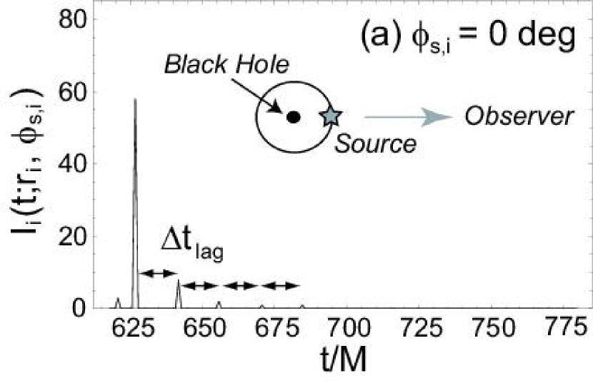
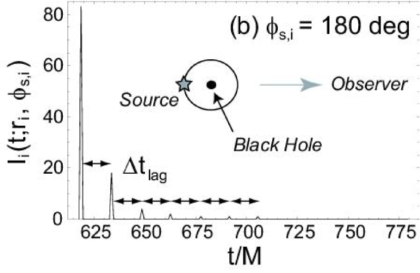
Figure 1: Sample signals from two random X-ray bursts (out of a total of $N_{b}=6000$) at (a) $\phi_{s,i}=0^{\circ}$ and (b) $\phi_{s,i}=180^{\circ}$ for $a/M=0.99$ and $r_{s}=r_{\rm ms}$. In each phase $N_{\rm ph}=200,000$ photons are isotropically emitted. Arrows indicate a roughly constant time lag $\Delta t_{\rm lag}/M\simeq 14$. Relative positions of the observer, source and the black hole are illustrated.

In fact, Figure 2 encapsulates the essence of the effect discussed herein: Because of the frame-dragging effects for a source within the ergosphere, even those photons with negative angular momenta (going backward in the local frame with respect to the hole’s rotation) are forced to propagate in the same sense as the rotating hole (the photon escaping directly to the observer in the upper right quadrant of Fig. 2 is one of them). All other photons can reach the observer (at phase $\phi_{s,i}=0^{\circ}$ in Fig. 2) only by moving in the direction of the hole’s rotation; as such they can do so by moving by an angle that is a fraction $q$ of $2\pi$ ($q=0$ for dashed ray; $q=1$ for gray ray, and $q=2$ for solid dark ray) to produce the response of Figure 1a. As we show explicitly in the next section, it is the constancy of this time-lag that is responsible for the presence of QPOs in the system. Such a constant lag is almost absent, however, for photon sources outside the ergosphere or in the Schwarzschild geometry, leading to qualitatively different results in these cases.

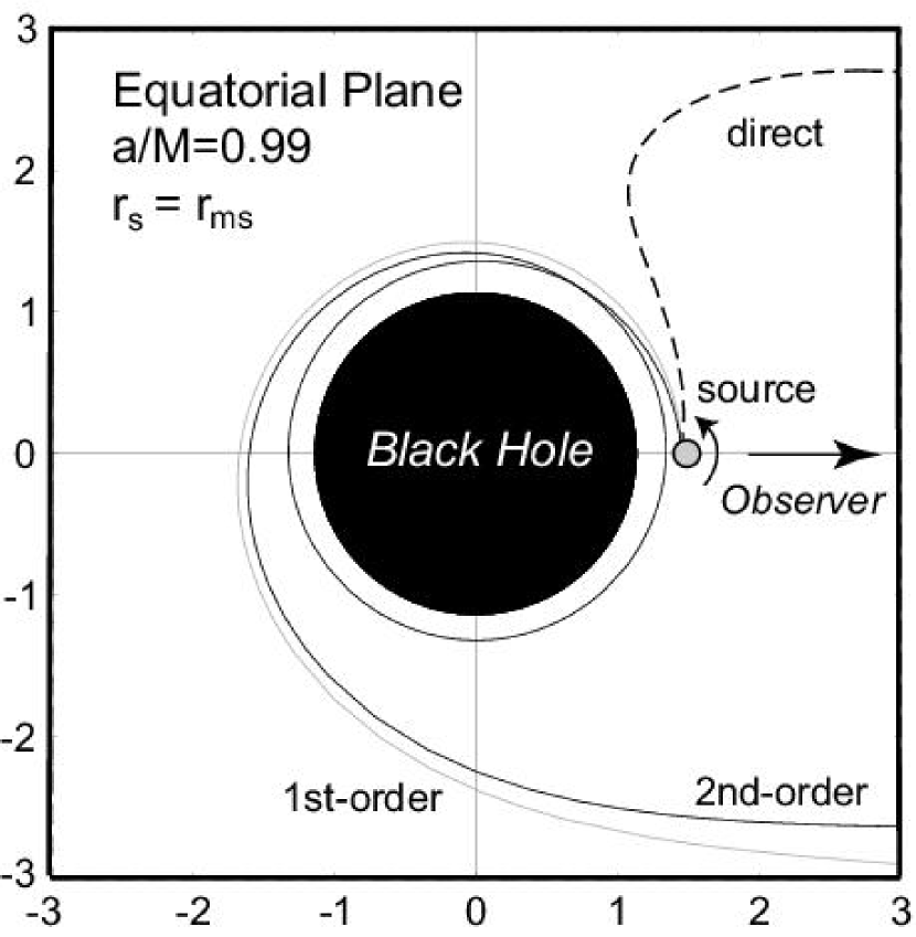
Figure 2: Representative photon rays corresponding to the response function in Figure 1a. The trajectory in the upper right quadrant (dashed curve) is a backward emitted photon. The gray and dark curves (solid curves) represent photons that reach the observer after $2\pi$ and $4\pi$ radians, respectively.

To be sure, even in the Schwarzschild geometry one expects that some photons can reach the observer after going around the hole by an angle that is an integer-multiple of $2\pi$, but their number is much too small to make an observable contribution to the response function. In support of this claim we present similar computations in a Schwarzschild geometry in which the frame-dragging effect is absent and the marginally stable orbit is larger ($r_{\rm ms}/M=6$). The response functions for (a) $\phi_{s,i}=90^{\circ}$ and (b) $165^{\circ}$ are depicted in Figure 3 for $N_{\rm ph}=200,000$ photons. It is apparent that the response function in this case comprises a very large peak at time $t/M\simeq 610$, a much smaller one at $t/M\simeq 632$ and two additional even smaller ones separated from this last one by $\Delta t_{\rm lag}/M\simeq 16$ and $\Delta t_{\rm lag}/M\simeq 32$ respectively, i.e indicating the presence of a constant lag in this particular phase too. In order to get a better understanding of the orbits responsible for these peaks and their relation to the corresponding orbits of the Kerr geometry we did obtain and plot in Figure 4 the orbits of the photons corresponding to these peaks. Thus the largest peak corresponds to photons that arrive at the observer directly from the source (in the retrograde direction with respect to the source direction), while the smaller one from photons that go around the hole by an angle $\Delta\phi\simeq 3\pi/2$ in the prograde direction. The next much smaller peak at $t/M=632+16$ is due to photons that arrive at the observer after going around the hole by an angle $\Delta\phi\simeq 5\pi/2$ in the retrograde direction and the one at $t/M=632+32$ after an angle $\Delta\phi\simeq 7\pi/2$ in the prograde direction. As the azimuthal angle $\phi_{s,i}$ approaches 180^∘, both the two largest and two smallest peaks move closer (as expected by symmetry) to obtain approximately the same normalization and merge for $\phi_{s,i}\simeq 180^{\circ}$, indicating that their time-lag is in fact not constant but depends strongly on the value of the phase angle $\phi_{s,i}$, unlike the situation for the Kerr geometry of Figure 1, where the lags are independent of the source phase. This is a crucial point in our model.

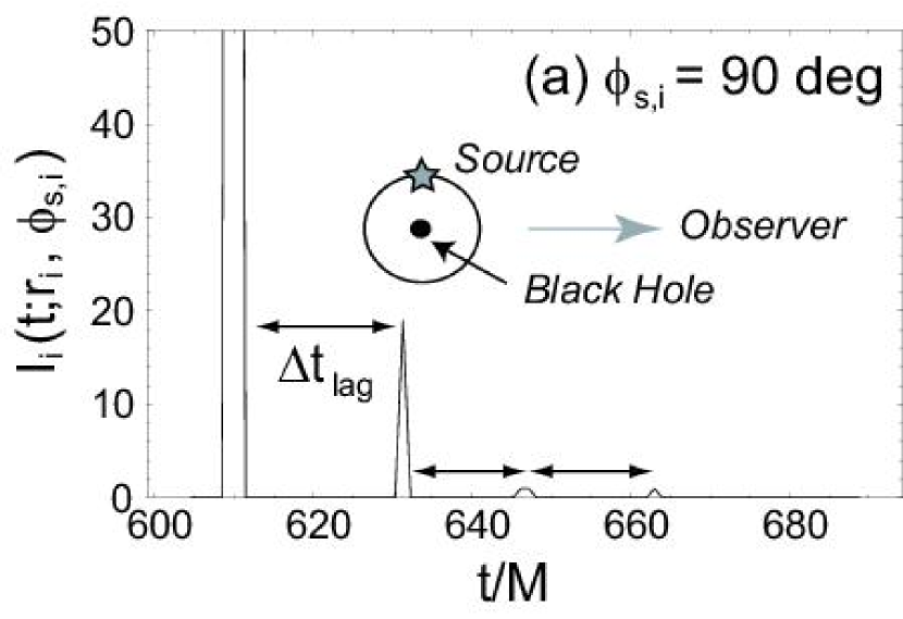
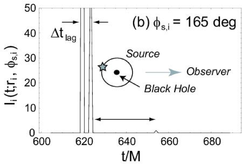
Figure 3: Same as Figure 1 but for $a/M=0$ and $r_{s}=r_{\rm ms}=6M$. No constant time-lag is seen.

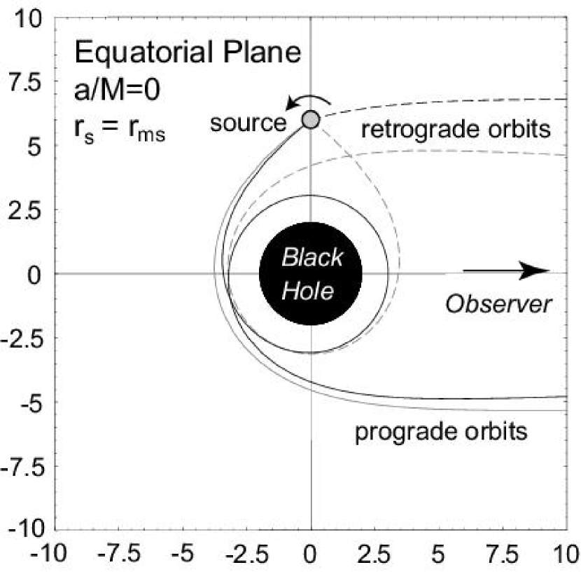
Figure 4: Representative photon rays corresponding to the response function in Figure 3a. The trajectories in the upper right quadrant (dashed curves) are backward emitted photon. The gray and dark curves (solid curves) represent photons that reach the observer after $\pi+\pi/2$ and $3\pi+\pi/2$ radians, respectively.

3 Model X-ray Light Curves and Timing Analysis

We have used the response function constructed as above to produce synthetic light curves. In order to avoid the introduction of QPO features by the rotation of the emitting sources, we have made the flare emission instantaneous and positioned the sources at random values of $\phi_{s,i}$, uniformly between 0 and $2\pi$; we also introduced the flares randomly in time using the following prescription of the time interval $\Delta T_{i}$ between the $i$-th and $(i+1)$-th bursts

$$\Delta T_{i}\equiv\bar{T}\times|\ln\left\{\rm{rnd}\left(0,1\right)\right\}|\ ,$$ (7)

where $\bar{T}$ is a mean timescale between bursts and $\rm{rnd}(0,1)$ denotes a random number between $0$ and $1$. We have chosen $\bar{T}\equiv fT_{\rm orb}$ where $T_{\rm orb}(r_{s})\equiv 2\pi(r_{s}^{3/2}+aM^{1/2})/M^{1/2}$ is the Keplerian orbital period at $r=r_{s}$ and $f$ ($f\sim 1$) characterizes the frequency of burst occurences relative to the orbital period $T_{\rm orb}$ (the precise value of $f$ is in fact not relevant for the shape of the power spectrum we are interested in).

Each burst produces a characteristic signal $I_{i}(t;r_{s},\phi_{s,i})$ unique to that specific azimuthal position $\phi_{s,i}$ with $I_{i}(t;r_{s},\phi_{s,i})$ denoting the intensity of the signal of the $i$-th burst as shown in Figures 1 and 3. The entire bolometric light curve then is the incoherent superposition of similar signals corresponding to the randomly produced flares, i.e.

$$I(t;r_{s})\equiv\sum_{i=1}^{N_{b}}I_{i}(t;r_{s},\phi_{s,i})\ ,$$ (8)

where $N_{b}$ (set to be 6,000) is the total number of X-ray bursts used in a given model light curve. Note that each flash contains $N_{\rm ph}=200,000$ photons.

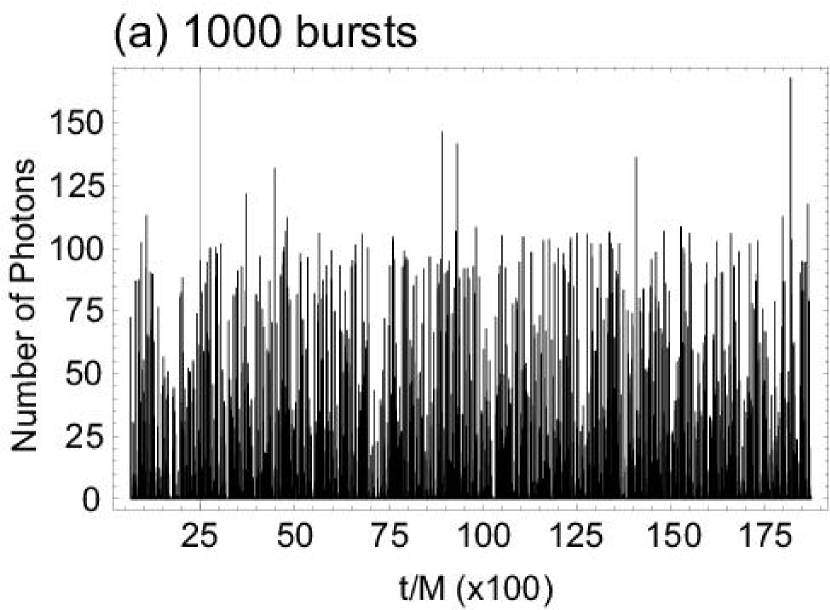
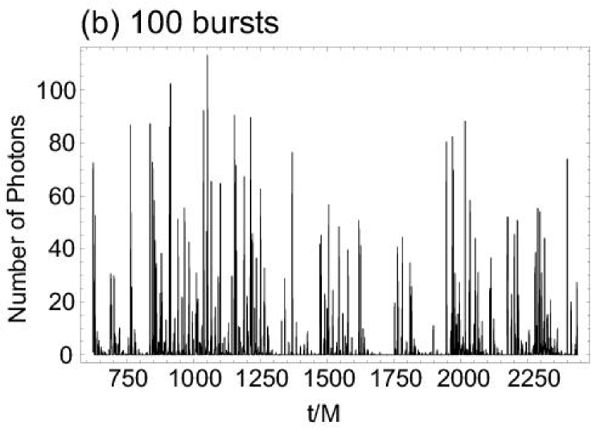
Figure 5: Two sample light curves generated as discussed in the text. (a) The light curve of a series of $N_{b}=1000$ bursts from sources at radius $r=r_{\rm ms}=1.45M$ for a black hole with $a/M=0.99$ and $f=1$. (b) The light curve of only the first 100 bursts of the same series. It is apparent that these are totally random.

Using the above prescription we have produced sets of model light curves varying the parameters $N_{b}$ and $f$ for the same values of the black hole parameters used to produce Figures 1 and 3. The simulated light curve seen by the observer is shown in Figure 5 where $N_{b}=1000$ bursts are considered in (a) and the first 100 bursts are extracted from (a) in (b). They exhibit no apparent periodicity, given the random positions $\phi_{s,i}$ and times of the induced flares $\Delta T_{i}$. We find that the characteristic appearance of the light curve essentially remains the same for the Schwarzschild cases too.

We have then used standard analysis tools for the Fourier transform $F(\omega)$ to produce the PDS $|F(\omega)|^{2}$ of these light curves along with the Autocorrelation Function (ACF) $R(\tau)$. These are shown in Figure 6 for various source radii, i.e. $r_{s}>r_{\rm ms},~{}r_{s}=r_{\rm ms}$ and a plunging orbit with $r_{s}<r_{\rm ms}$, for a black hole with $a/M=0.99$. A characteristic peak is clearly seen in the PDS at angular frequency of $\omega_{\rm QPO}M\sim 0.4$ and its higher multiple modes, which for $M=10M_{\odot}$ corresponds to a peak frequency $\nu_{\rm QPO}\sim 1.3-1.4$ kHz. The ACF exhibits also a prominent peak at the equivalent time lag of $\tau/M\sim 14-15$ and perhaps encapsulates better the underlying physics behind the QPO, i.e. the presence of a well-defined time lag (i.e. an “echo”) in the response of this system. This is best seen, e.g., in Figures 6a-d. The QPO pattern (peak frequency and width) remains essentially the same regardless of the source position, as long as it is within the ergosphere. On the other hand, as $r_{s}$ approaches the static limit ($r=r_{\rm static}=2M$ near the equator), the QPO signal begins to disappear (see Figs. 6e and f), since the time-lags between the peaks of the response function is no longer constant, as discussed earlier.

It should be noted that the choice of the times of flare injection [equation (7)] guarantees that in the absence of the lags discussed above the corresponding PDS would be just white noise. However, because our timing resolution in this numerical experiment is $M$, we have approximated each “bunch” of photons received at a given angle and a given resolution interval as a Gaussian of area normalized to the number of photons received in each interval and FWHM equal to $M$. It is precisely this finite width of our “shots” that leads to the high frequency cut-off of the PDS given in Figures 6a-d. Of course, at the low frequencies the PDS is that of white noise.

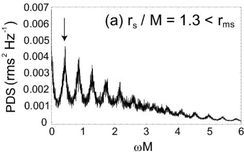
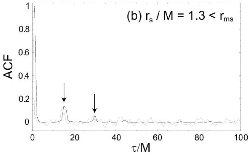
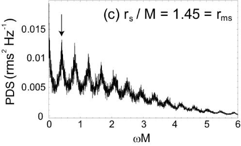
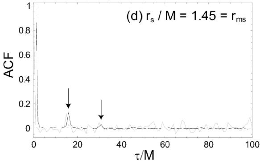
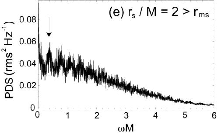
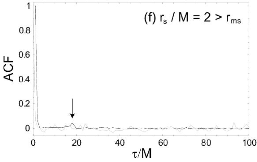
Figure 6: Timing analysis of random X-ray bursts with $a/M=0.99$ for $r_{s}/M=1.3$ (top rows), $1.45$ (middle rows) and $2$ (bottom rows). We set $N_{b}=6000$. Left columns show the average power density spectra (PDS) while right columns show the corresponding autocorrelation functions (ACF). In the ACF we show two cases: $N_{b}=6000$ (dark curves) and $100$ (gray curves) for comparison.

In order to study quantitatively the QPO feature in this model we have also examined its dependence on the black hole rotation $a$ for $r_{s}=r_{\rm ms}$ in Figure 7. To do so we select two values for the black hole spin, namely $a/M=0.995$ and $a/M=0.9428$. The first was chosen to verify that the effect becomes more prominent with the increase of the black hole spin; the second value was chosen by the requirement that the equatorial boundary of the ergosphere be equal to that of the ISCO, i.e. that $r_{\rm ms}=r_{\rm static}=2M$. The first case yields clearly prominent QPO and peaks at the appropriate lags in the ACF. However, these features become almost statistically insignificant as the spin parameter approaches the critical value of $a/M=0.9428$ (for which $r_{s}=r_{\rm ms}=r_{\rm static}$) for the reasons discussed in the previous paragraphs of this section.

We have also performed a similar calculation for a Schwarzschild black hole case for $r_{s}=r_{\rm ms}=6M$ to examine whether the QPO features we have found in Kerr geometry may also be produced in the absence of black hole rotation. In this case the PDS (not shown here) exhibits no QPO features similar to those of the Kerr case (as expected). The reason is the absence of a constant time-lag between the two major peaks of the response function (see Fig. 3); the normalization of the two minor peaks is just too small to make a difference in the PDS, despite the presence of roughly constant lags between them at some phases. The corresponding ACF also showed no particular coherent timescale. We have repeated similar computations for various source radii ($r_{s}\gtrsim r_{\rm ms}$ and $r_{s}<r_{\rm ms}$) for Schwarzschild case and found that in no case the QPO features seen above were produced. As discussed above this is due to the absence of a constant time lag in the system response. We will come back to discuss this issue in §4. Of course, should there be a reason that a particular phase is favored as the site of the X-ray flares considered by our model, then one would expect QPOs to be present for sources in a Schwarzschild geometry too.

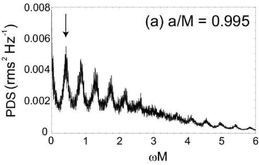
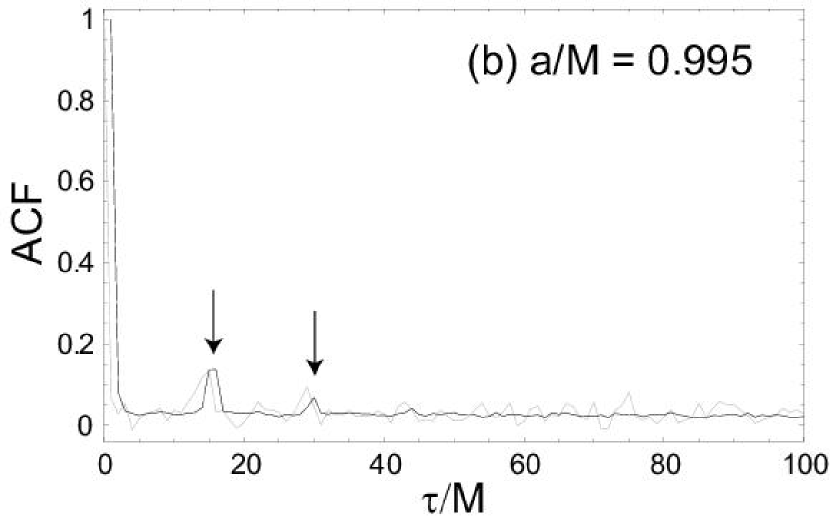
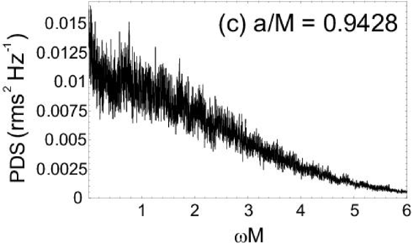
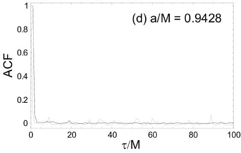
Figure 7: Same as Figure 6 but for $a/M=0.995$ (top columns) and $0.9428$ (bottom columns) with $r_{s}=r_{\rm ms}(a)$.

Finally, we have checked that the feature obtained is not simply an artifact due to photon statistics by changing the number of bursts and the random number sequence used and indeed nearly identical results were consistently found. Note that for a given black hole rotation $a$, there are no free parameters other than the radial position of the flares $r_{s}$, and the mean timescale of each burst $\bar{T}$, neither of which changes the value of the lag in the response function.

4 Discussion

We have presented above a process that can lead to QPO features in the PDS of accreting black hole systems. This process is to a certain extent different from the typical QPO models in the literature in that it relies on the “echo” of a (however random) signal for the emergence of the QPO in the observed PDS. By contrast, most QPO models invoke the presence of an underlying (but perhaps obscured due to noise) oscillation in the emitted photon flux. Whether this qualifies it as an alternative QPO model or not is, in our view, a matter of convention. However, it provides a mind-set concerning the QPO phenomenon that deviates from that of the more conventional considerations which may lead to novel future insights on the subject. The difference of these two distinct QPO notions is perhaps exemplified best mathematically by the corresponding ACF, which in one case has an oscillatory behavior while in the other the double peak form presented in Figures 6 and 7.

As discussed in the previous section, the “echo” of the proposed model is the result of the black hole angular momentum $a$ and the ensuing dragging of inertial frames on the trajectories of the photons emitted within its ergosphere; as such, this “echo” is absent in black holes of sufficiently small values of $a$. This is not the first time that frame-dragging has been invoked to account for a certain aspect of the QPO phenomenon. For example, the same effect and the accompanying Lense–Thirring disk precession has been invoked to account for the dependence of the intrafrequency correlations of several low frequency QPOs (Stella & Vietri, 1998; van der Klis, 2000; Schnittman et al., 2006); the effect we describe herein is different in that it affects the orbits of individual photons, rather the orientation of the entire disk.

One should further note that, because the “echo” lags that produde these QPOs depend only on the background geometry of the accreting black hole (they are roughly equal to the length of the circular photon orbit for this geometry), they (and also the resulting QPO frequencies) are independent of the source flux (the accretion rate). On the other hand, given that the QPOs of accreting neutron stars and most of the QPOs of accreting black holes do depend, in general, on the source flux (van der Klis, 2000), they are likely due processes different from that described above. Nonetheless, as discussed in §1, QPOs that do not depend on the source flux have been discovered in a number of galactic black hole candidates (Strohmayer, 2001a, b). However, the frequencies of these latter QPOs are much too small ($\nu_{\rm QPO}\sim 100-400$ Hz) to be attributed to the process described herein [$\nu_{\rm QPO}\simeq 1400\,(10M_{\odot}/M)]$, unless our understanding of strong gravity physics is in significant error.

Up to this point, the discussion of our model considered flares whose duration is much shorter than the orbital period of the accretion disk near its ISCO. Clearly, the “echo” process discussed herein is present for longer flare durations, even if the latter exceeds the local orbital period. However, in this case the model becomes very similar to those of orbiting hot spots discussed earlier Karas (1999); Schnittman (2005). We have produced a number of model light curves assuming the flare duration to be several times the ISCO orbital period (i.e. just like in the orbiting hot spot model) and computed the corresponding PDS and ACF. In this case, the geometrical echo, while still present, makes only a small contribution to the PDS, whose QPOs are now dominated by the orbiting hot spot periodic motion.

While the process we discussed above is quite robust (it depends only on the geometry of the accreting object), its potential observability depends on a number of factors. To begin with, our calculations were performed exclusively on the equatorial plane of a Kerr black hole; therefore, our present results are valid only for disks that are geometrically thin and for observers at relatively low latitudes. For observers at moderately higher latitudes (or thick disks), our orbit calculations have to be supplemented with those for the $\theta-$coordinate (to follow the poloidal motion) that have been omitted so far in this work. However, the essence of the effect we discussed above, i.e. forward thrust of all photon trajectories produced within the ergosphere, whether equatorial or not, is expected to be present in that case too and thus qualitatively we expect the same phenomenon to be conditionally observable for non-equatorial source/observer configurations. Our preliminary calculations indicate the presence of such QPO for observers at latitudes at least as high as $\sim 30^{\circ}$ from the disk mid-plane. Quantitative analysis of this aspect of the problem, which bears the application of these ideas to thick disks, will be presented in a future publication.

Another limitation of the model discussed in the earlier sections is that of the source radius $r_{s}$. The response frames of Figure 1 were computed assuming the source to be on the ISCO at $r_{s}/M\simeq 1.45$. Changing the source radius leads to a quantitatively similar behavior, i.e. the ACF still exhibits a peak at the same value of the lag $\tau/M\simeq 14$, as long as the source of photons is located within the static limit (ergosphere), i.e. for $r_{s}/M\mathrel{\raise 1.29167pt\hbox{$<$}\mkern-14.0mu\lower 2.58334pt\hbox{$\sim$}}2$ near the equatorial plane. Interestingly, for the value $a/M=0.99$ used in these calculations the ACF peak at $\tau/M\simeq 14$ disappears gradually as the source radius increases past $r_{s}/M\mathrel{\raise 2.15277pt\hbox{$>$}\mkern-14.0mu\lower 2.58334pt\hbox{$\sim$}}2$, i.e. as the source moves outside the ergosphere, a fact which suggests that the effect we have presented is in fact due to the strong dragging of inertial frames. Equivalently, we anticipate the gradual disappearance of this peak in the ACF as the value of the black hole spin $a$ decreases down to a critical value of $a/M\sim 0.9428$ (where the radius of ISCO becomes equal to that of static limit) and the ergosphere shrinks to leave much of the disk outside. While the frame-dragging is still operative even at radii outside the static limit, it is simply not effective enough to cause significant azimuthal beaming.

We have in fact checked that the effect we consider is not due to the source proximity to the horizon (a situation possible without free fall onto the hole only if the latter is rapidly rotating) by computing the orbits of photons from radii as small as $r_{s}/M\simeq 2.1$ by matter in-falling (in the plunging region of $r_{s}<r_{\rm ms}$) onto a Schwarzschild black hole. In computing the photon orbits in this last case we have taken into account all the components of the velocity of the in-falling plasma, calculated by assuming that it began its in-fall from the ISCO. Plunging gas thus preserves its ISCO energy and angular momentum. We found that for flares that take place close to the horizon ($r_{s}/M\sim 2.1$) most photons end up into the black hole (as expected); however, the behavior of the response of the escaping photons in no case gave us the constant time-lag obtained in the rapidly rotating black hole case, to produce QPO features in the PDS. In the case of a Schwarzschild black hole, an (unstable) photon circular orbit lies at $r_{s}=3M<r_{\rm ms}$ inside the plunging region, from which radius one would expect higher-order photons (multiple orbit photons). However, since the plunging X-ray sources also possess significant radial velocity component at this radius close to the horizon, many photons emitted at $r_{s}/M=3$ are Doppler-beamed in the direction of the source motion. The radial beaming effect therefore keeps most of the photons from being emitted in an azimuthal direction, effectively suppressing their multiple orbits.

Finally, to explore even the most likely case to produce QPOs in a Schwarzschild geometry, we computed the response function of the system for a source at an unstable (Keplerian) circular orbit at $r/M=3.001$. At this radius, the high rotational speed of the source ($v\simeq 0.9995c$) produces effects similar to the dragging of inertial frames, because most photons are beamed in the forward direction by the source rotation. The corresponding response function and photon orbits for a source at $\phi_{s,i}\simeq 90^{\circ}$ are given in Figures 8a,b, while the corresponding PDS and ACF in Figures 9a,b. As it can be seen there, for this specific source position, most photons reach the observer after going around the black hole by $\Delta\phi\simeq 3\pi+\pi/2$ while the fraction that reaches after $\Delta\phi\simeq\pi+\pi/2$ is comparable but smaller; there are also a small number of photons that reach the observer in the counter clockwise direction after $\Delta\phi\simeq 2\pi+\pi/2$; photons that reach the observer after a larger number of rotations are not discernible at this resolution. However, as the source phase $\phi_{s}$ changes, while the lag between the major peaks remains roughly constant, the relative normalization shifts quickly and for most of phases the response is dominated by a single peak. This fact, along with the random choice of the phase of a given burst of our light curve prescription, “washes-out” potential QPO features, leading to the PDS shown in Figure 9a. On the contrary, in the Kerr case, the frame-dragging aided azimuthal beaming helps a significant fraction of the photons orbit around the black hole for all values of the phase angle $\phi_{s}$. This is an essential difference between Schwarzschild and Kerr black hole cases, which we conclude is manifested as the QPO feature we see here.

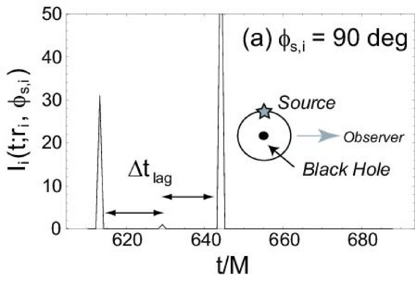
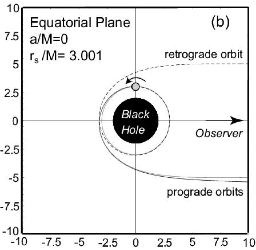
Figure 8: (a) The response function for a source at an unstable (Keplerian) circular orbit at $r_{s}/M=3.001$ at a phase $\phi_{s}=90^{\circ}$. The two large peaks correspond to the prograde orbits that cover angles $\Delta\phi=\pi+\pi/2$ and $3\pi+\pi/2$ respectively. The small peak at midpoint corresponds to the retrograde orbit that covers an angle $\Delta\phi=2\pi+\pi/2$. (b) The photon orbits corresponding to the features of the figure on the left.

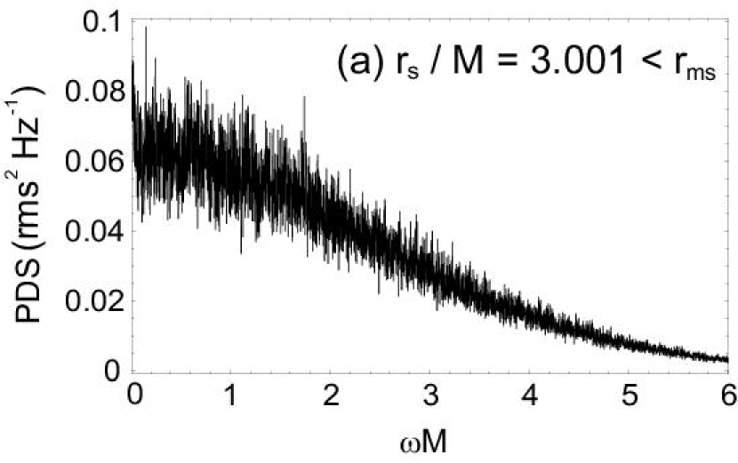
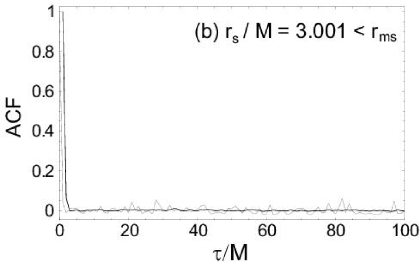
Figure 9: Predicted PDS of the light curve of a source at $r_{s}/M=3.001$ obtained using the response function of Figure 8 and the prescription given in the text. (b) The ACF of the same light curve for $N_{b}=6000$ (dark curves) and $N_{b}=100$ (light curves).

Up to this point we have only considered the time correlations between the photons emitted by the accretion disk without any reference to their energy. However, if these photons are of a specific energy (i.e. the Fe transitions observed in accretion disks), there exists a relation (redshift) between the emitted and the received photon energies given by

$$g\equiv\frac{\nu_{\rm rec}}{\nu_{\rm emt}}=\frac{\left(r_{s}^{2}\Delta_{s}/A_{s}\right)^{1/2}\left(1-v_{s}^{2}\right)^{1/2}}{\left(1-b\Omega_{K}\right)}\ ,$$ (9)

where $\Omega_{K}$ is the Keplerian angular frequency, and $v_{s}$ is the azimuthal component of the X-ray source velocity measured in LNRF. It would therefore be of interest to consider, in addition to the time correlations, also their additional dependence on the photon energy (or energy shift factor) $g$; the impetus for such a study comes from the observed energy dependence of the geometry attributed QPOs in GRO J1655-40 (e.g. Strohmayer, 2001a). We hope to look into this as well as the above unresolved issues in a future publication.

We would like to conclude with some general remarks concerning the “light echo” responsible for the QPOs presented in this paper: This is a very generic process and would be present at any source that exhibits a delay in its response function, not necessarily the one we described in this note. The same point has been made earlier (Kazanas & Hua, 1999) in a different context and we believe that it may have broader applicability. It should be noted, in this same context, that the response of an axisymmetric disk does not exhibit any such features, however, the response of a warped disk (e.g. Hickox & Vrtilek, 2005) should; therefore such disks may exhibit QPO features of the kind described herein at the periods comparable to the light crossing time across the disk, features that maybe worth searching for in the data.

Finally, we would like to point out that the lack of apparent phase coherence in this model makes the PDS quite noisy and therefore we expect that the detection of such features may require their search in the light curves of higher mass objects that would push the corresponding frequencies to lower values that are easier to detect (perhaps intermediate mass black holes associated with ULXs or nearby AGN), using low background, high throughput missions like Constellation-X.

5 Appendix

In this Appendix we show the definition of the local angle $\delta$ of photon emission in LNRF and its relation to photon’s impact parameter $b$ (which is defined as specific angular momentum). We then explicitly derive radial component of the geodesic equation in terms of $\delta$ which we have integrated in producing Figures 2, 4 and 8 in §2 and 3. First, toroidal velocity of (either a massive or a massless) particle seen by a local observer in LNRF of Kerr metric is given by

$$v^{\hat{r}} = \frac{A^{1/2}}{\Delta}\frac{\dot{r}}{\dot{t}}\ ,$$ (10)

$$v^{\hat{\phi}} = \frac{A}{\Delta^{1/2}\Sigma}\left(\frac{\dot{\phi}}{\dot{t}}-\omega\right)\ ,$$ (11)

where we restrict ourselves to equatorial trajectories ($\theta=\pi/2$) in the disk plane. In this frame the photon emission angle $\delta$ between the propagation direction and the radial direction (e.g. Misner et al., 1973, p. 675) is defined as

$$\cot\delta\equiv\frac{v^{\hat{r}}}{v^{\hat{\phi}}}=\frac{\Sigma}{(A\Delta)^{1/2}}\frac{\dot{r}}{\dot{\phi}-\omega\dot{t}}\ .$$ (12)

On the other hand, radial component of the geodesic equation is given by

$$\Sigma^{2}\dot{r}^{2}=R(r)\ ,$$ (13)

where $R(r)=(r^{2}+a^{2}-ab)^{2}-\Delta(b-a)^{2}$ for equatorial trajectories and $b$ is photon’s impact parameter. With the help of equations (3) and (4) one can express $b$ in terms of $\dot{r}$ and $\delta$ as

$$b(\dot{r},\delta) = \dot{r}\left(\frac{r\xi}{\Delta}\right)^{1/2}\tan\delta\ .$$ (14)

Substituting equation (14) into equation (13) one obtains an explicit expression for $\dot{r}$ in terms of the local angle $\delta$ only as

$$\dot{r}_{\pm}(\delta) = \frac{\xi^{1/2}\cos^{2}\delta\left(\pm r\Delta|\sec\delta|-2aM\Delta^{1/2}\tan\delta\right)}{r^{1/2}\left[r^{3}(r-2M)+a^{2}(r^{2}-2M^{2})+2a^{2}M^{2}\cos(2\delta)\right]}\ ,$$ (15)

which is equation (5), and the sign in the numerator depends on the direction of photon emission in the rest-frame of fluid/source. Correspondingly, equation (14) is now rewritten as

$$b_{\pm}(\delta) = \frac{\xi\sin(2\delta)[\pm r\Delta|\sec\delta|-2aM\Delta^{1/2}\tan\delta]}{2\Delta^{1/2}\left[r^{3}(r-2M)+a^{2}(r^{2}-2M^{2})+2a^{2}M^{2}\cos(2\delta)\right]}\ .$$ (16)

References

- Abramowicz & Kluźniak (2001) Abramowicz, M. A., & Kluźniak, W. 2001, A&A, 374, L19
- Kluźniak & Abramowicz (2001) Kluźniak, W., & Abramowicz, M. A. 2001 (astro-ph/0105057)
- Aoki et al. (2004) Aoki, S. I., Koide, S., Kudoh, T., Nakayama, K., & Shibata, K. 2004, ApJ, 610, 897
- Aschenbach (2004) Aschenbach, B. 2004, MNRAS, 425, 1075
- Chandrasekhar (1983) Chandrasekhar, S. 1983, The Mathematical Theory of Black Holes (Oxford: Oxford Univ. Press)
- Cui et al. (1998) Cui, W., Zhang, S. N., & Chen, W. 1998, ApJ, 492, L53
- Cui et al. (1999) Cui, W., Zhang, S. N., Chen, W., & Morgan, E. H. 1999, ApJ, 512, L43
- Czerny & Goosmann (2004) Czerny, B., & Goosmann, R. 2004, A&A, 428, 353
- Donmez (2007) Donmez, O. 2007, Modern Physics Letters A, 22, 02, 141
- Fukumura et al. (2007) Fukumura, K., Takahashi, M., & Tsuruta, S. 2007, ApJ, 657, 415
- Fukumura & Kazanas (2007) Fukumura, K., & Kazanas, D. 2007, ApJ, 644, 14
- Galeev et al. (1979) Galeev, A. A., Rosner, R., & Vaiana, G. S. 1979, ApJ, 229, 318
- Haardt et al. (1994) Haardt, F., Maraschi, L., & Ghisellini, G. 1994, ApJ, 432, L95
- Hickox & Vrtilek (2005) Hickox, R. C., & Vrtilek, S. D. 2005, ApJ, 633, 1064
- Karas (1999) Karas, V. 1999, PASJ, 51, 317
- Kazanas & Hua (1999) Kazanas, D. & Hua, X.-M. 1999, ApJ, 519, 750
- Kato (2001) Kato, S. 2001, PASJ, 53, 1
- Lense & Thirring (1918) Lense, J., & Thirring, H. 1918, Phys. Z., 19, 156
- Misner et al. (1973) Misner, C. W., Thorne, K. S., & Wheeler, J. A. 1973, in Gravitation, Freeman, San Francisco
- Nayakshin & Kazanas (2001) Nayakshin, S., & Kazanas, D. 2001, ApJ, 553, L141
- Novikov & Thorne (1973) Novikov, I. D., & Thorne, K. S. 1973, in Black Holes, ed. C. DeWitt and B. DeWitt (Gordon and Breach, New York)
- Nowak et al. (1997) Nowak, M. A., Wagoner, R. V., Begelman, M. C., & Lehr, D. E. 1997, ApJ, 477, L91
- Page & Thorne (1974) Page, D., & Thorne, K. S. 1974, ApJ, 191, 499
- Poutanen & Fabian (1999) Poutanen, J., & Fabian, A. C. 1999, MNRAS, 306, L31
- Schnittman & Bertschinger (2004) Schnittman, J. D., & Bertschinger, E. 2004, ApJ, 606, 1098
- Schnittman (2005) Schnittman, J. D. 2005, ApJ, 621, 940
- Schnittman et al. (2006) Schnittman, J. D., Homan, J., & Miller, J. M. 2006, ApJ, 642, 420
- Stella & Vietri (1998) Stella, L., & Vietri, M. 1998, ApJ, 492, L59
- Strohmayer (2001a) Strohmayer, T. E. 2001, ApJ, 552, L49
- Strohmayer (2001b) Strohmayer, T. E. 2001, ApJ, 554, L169
- Strohmayer et al. (2007) Strohmayer, T. E., Mushotzky, R. F., Winter, L., Soria, R., Uttley, P., & Cropper, M. 2007, ApJ, 660, 580
- van der Klis (2000) van der Klis, M. 2000, ARA&A, 38, 717