1 Introduction

The X-ray emission lines from O stars are wind-broadened but are surprisingly symmetric. Asymmetry should arise due to the preferential absorption of red-shifted photons, which are produced on the far side of the wind and seen through a larger column density of cold, absorbing material. The very modest asymmetry in the observations implies that mass-loss rates are lower than has been presumed, which is, of course, in line with other recent observations. Alternatively, it has been suggested that the mass-loss rates are actually high, but the effective opacity of the wind is reduced due to porosity, or macroclumping (Oskinova et al. [2006]).

In this very brief paper, in which we focus on one strong representative line in the Chandra grating spectrum of $\zeta$ Pup, we explore whether the measured profile shapes can discriminate between mass-loss reduction and porosity. Even if they cannot, by fitting models to data we can quantitatively explore the trade-off between the key parameters: fiducial optical depth, $\tau_{\ast}\equiv\kappa\dot{M}/4{\pi}v_{\infty}R_{\mathrm{\ast}}$, and the terminal porosity length, $h_{\rm\infty}$. Here we do this by fitting the Owocki & Cohen ([2001]) profile model to one strong line in the Chandra HETGS/MEG spectrum of $\zeta$ Pup. We then fit a modified profile model, where the opacity is adjusted for porosity according to Owocki & Cohen ([2006]).

2 Fitting Models to the Data

There are 560 counts in the Fe XVII line shown in Fig. 1, accumulated during an exposure time of 68 ks. The line is well resolved and clearly asymmetric, with the characteristic blue shifted and skewed line shape that is expected from a spherically symmetric, beta-velocity wind with embedded X-ray emission and continuum absorption from the cool, dominant component of the wind. The first model we fit to the data is the simplest – a non-porous Owocki & Cohen ([2001]) model where the optical depth depends on the atomic opacity. We note that this model does not preclude microclumping of the sort that affects density-squared emission diagnostics, but does not affect column-density based diagnostics like X-ray emission line profiles. However, this standard profile model does not include large scale porosity, or macroclumping, with $h\equiv{\ell}/f>r$, where $h$ is the porosity length, defined as the clump size scale to the volume filling factor (Owocki & Cohen [2006]). We do fit porous models later in this paper.

We fit the model, along with a fixed power-law continuum, within XSPEC, to the line over the wavelength range shown in Fig. 1. The fitting routine in XSPEC adjusts the free parameters of the model: $R_{\mathrm{0}}$, the radius below which there is no X-ray emission, $\tau_{\ast}$, the fiducial wind optical depth, and the normalization, until the global minimum of the fit statistic – here the C statistic (Cash [1979]), which is the maximum likelihood statistic for Poisson-distributed data – is found. The best-fit model, with $R_{\mathrm{0}}=1.5\pm.2\leavevmode\nobreak\ {\mathrm{R}_{\ast}}$ and $\tau_{\ast}=2.0\pm.5$, is plotted over the data in Fig. 1.

The uncertainties on the parameters can be estimated by evaluating ${\Delta}C$, the difference between the C statistic value for a given choice of parameters and that of the best-fit model. The distribution of ${\Delta}C$ is the same as that of ${\Delta}{\chi}^{2}$ and a specific value corresponds to a formal confidence limit. By drawing contours of constant ${\Delta}C$ in the parameter space of interest, we can see the extent of a given parameter’s possible range and the correlation between parameters, as we show in Fig. 2.

Figure 1: An Fe XVII emission line, formed in a thermal plasma at a few $10^{6}$ K, with Poisson error bars. The approximate spectral resolution is indicated by the orange bar. The best-fit non-porous model is shown.

Figure 2: These confidence contours in the $R_{\mathrm{0}}$ - $\tau_{\ast}$ parameter space of the fit of the non-porous model to the Fe XVII line, shown in Fig. 1, enclose 68%, 90%, and 95% of the model parameter space where the true model parameters lie, given the data and the assumed model.

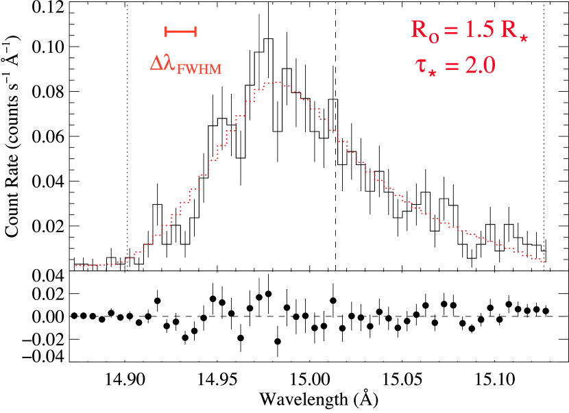
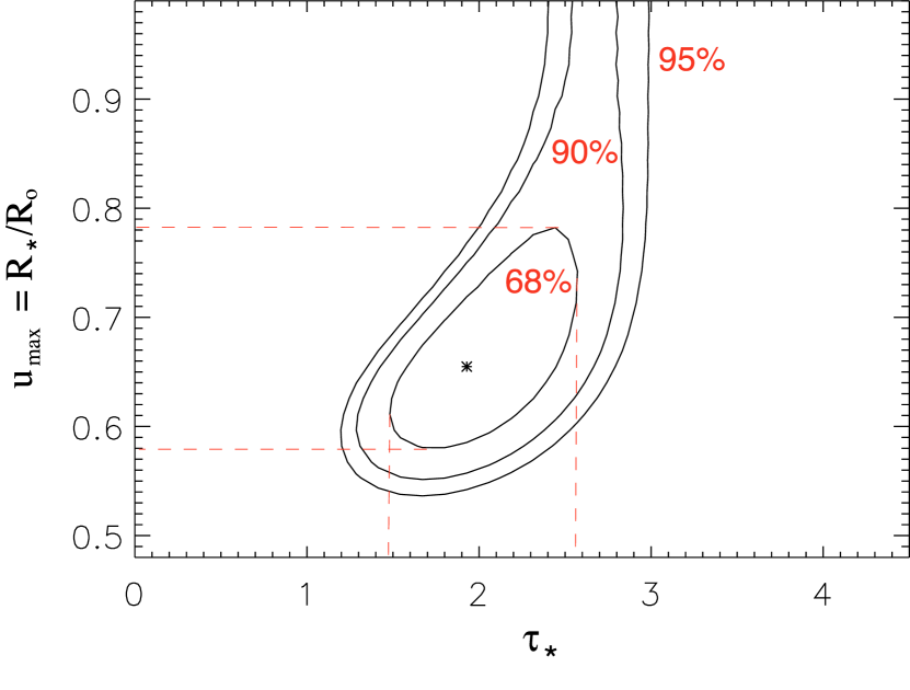
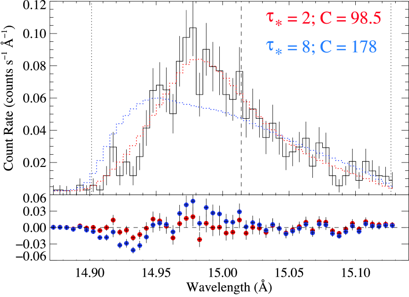
The value of $\tau_{\ast}$ we derive from the model fitting, $\tau_{\ast}=2.0\pm.5$, implies a mass-loss rate of $\dot{M}=1.5\pm.4\times 10^{-6}\leavevmode\nobreak\ \mathrm{M}_{\odot}\leavevmode\nobreak\ \mathrm{yr}^{-1}$, given an X-ray opacity at 15 Å of 70 cm² g^-1 (Waldron et al. [1998]). If, on the other hand, we take the mass-loss rate of $\zeta$ Pup to be $\dot{M}=6\times 10^{-6}\leavevmode\nobreak\ \mathrm{M}_{\odot}\leavevmode\nobreak\ \mathrm{yr}^{-1}$ and use $R_{\ast}=19\leavevmode\nobreak\ {\mathrm{R}_{\odot}}$ and $v_{\infty}=2250$ km s^-1 (Puls et al. [1996]), then we expect the wind to have a fiducial optical depth of $\tau_{\ast}=8$. The best-fit model is favored over a $\tau_{\ast}=8$ model with $>99.99$% confidence (${\Delta}C=79$). In Fig. 3 we show the optimal model with a fixed $\tau_{\ast}=8$ ($R_{\mathrm{0}}$ and normalization are free parameters) along with the global best-fit model.

Figure 3: The global best-fit non-porous wind model is shown in red and the best-fit model with the wind opacity expected based on the standard mass-loss rate is shown in blue.

Figure 4: Suite of porous line profile models, shown at infinite resolution. Within each panel, three optical depth values are represented, $\tau_{\ast}=1,2,8$: black, red, blue.

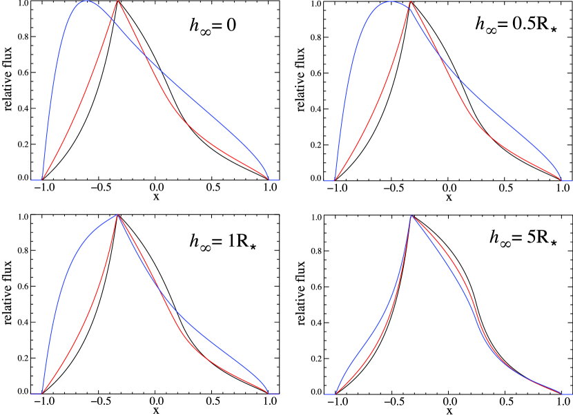
We next fit models that allow for porosity, but are otherwise identical to the Owocki & Cohen ([2001]) models fit in the previous subsection. In these porous models, the opacity is not atomic, but rather geometric, and due to optically thick clumps of size $\ell$ and filling factor $f$. The optical depth is thus modified according to ${\kappa}_{eff}={\kappa}(1-e^{-\tau_{c}})/\tau_{c}$, where $\kappa$ is the microscopic opacity and $\tau_{c}$ is the clump optical depth, $\tau_{c}=\kappa\ell\langle\rho\rangle/f$, where $\langle\rho\rangle$ is the local mean wind density (Owocki & Cohen [2006]). We parameterize the porosity length as $h(r)=h_{\infty}(1-R_{\ast}/r)^{\beta}$ and fix $\beta=1$, leaving the terminal porosity length, $h_{\infty}$ as the single additional parameter of the model. As can be seen in Fig. 4, porosity has only a weak effect, even at $h_{\infty}=1$. Values above unity are required before the profiles are strongly affected.

Now, by fitting this porous line profile model to the data, we can examine the joint constraints on the key parameters: $\tau_{\ast}$ and $h_{\infty}$, while allowing $R_{\mathrm{0}}$ and the normalization to also be free parameters of the model fit. When we do this, we find a best-fit terminal porosity length of $h_{\infty}=0.0$. In other words, the non-porous model is preferred over the porous one. In Fig. 5 we show the joint confidence limits on $h_{\infty}$ and $\tau_{\ast}$.

Figure 5: The 68%, 90%, and 95% confidence contours in $\tau_{\ast}$ - $h_{\infty}$ parameter space, with the best-fit global model shown as the red star. The green star is the location of the optimized model with $\tau_{\ast}=8$ fixed at the value implied by the literature mass-loss rate. The green line denotes the 68% confidence range on the terminal porosity length, $h_{\infty}$ when $\tau_{\ast}=8$. The vertical red line emphasizes that even with $h_{\infty}=1$, the wind optical depth is only a little higher than the non-porous value of $\tau_{\ast}=2.0$.

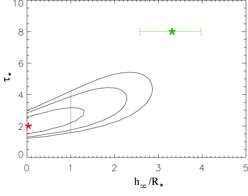
From this figure, we can see that the model with low optical depth and no porosity is preferred with a high degree of formal significance over the model with high optical depth and a large porosity length. We can also see, from the shape of the confidence contours, that the porosity length does not appreciably change the optical depth derived from the data until $h_{\infty}>{\mathrm{R}_{\ast}}$. This is in accord with the expectations from the sensitivity of the model profiles to the value of this parameter (as shown in Fig. 4).

We stress that the porous model with the higher mass-loss rate provides an adequate fit to the data, just not as good a fit as the non-porous model. It is possible that a porous model with a different description of porosity could fit the data as well as the non-porous model fit we show. However, we can definitively say two things from the model fitting we have reported on here: (1) Porosity cannot explain the only modestly asymmetric line profiles in $\zeta$ Pup any better than a non-porous model with a reduced mass-loss rate can; if anything, it provides a worse fit. And, (2) in order to fit the data with a high mass-loss rate, high porosity model, terminal porosity lengths of several $\mathrm{R}_{\ast}$ are required.

Regarding this last point, two-dimensional simulations of the line-driven instability show numerous very small structures, as the compressed shells created by the instability break up laterally. Constraints on moving emission bumps seen in WR winds using these 2-D simulations shows that the clumps subtend about 3 degrees, or 1/20 steradian, implying linear clump scales of 1/20 the local stellar radius, and thus quite small porosity lengths (Dessart & Owocki [2003, 2005]).

References

- 1979 Cash, W. 1979, ApJ, 228, 939
- 2003 Dessart, L., & Owocki, S.P. 2003, A&A, 406, L1
- 2005 Dessart, L., & Owocki, S.P. 2005, A&A, 437, 657
- 2006 Oskinova, L.M., Feldmeier, A., & Hamann, W.-R. 2006, MNRAS, 372, 313
- 2001 Owocki, S.P., & Cohen, D.H. 2001, ApJ, 559, 1108
- 2006 Owocki, S.P., & Cohen, D.H. 2006, ApJ, 648, 565
- 1996 Puls J., et al. 1996, A&A, 305, 171
- 1998 Waldron, W.L., Corcoran, M.F., Drake, S.A., & Smale, A.P. 1998, ApJS, 118, 217