Supercooling and phase coexistence in cosmological phase transitions
Abstract
Cosmological phase transitions are predicted by Particle Physics models, and have a variety of important cosmological consequences, which depend strongly on the dynamics of the transition. In this work we investigate in detail the general features of the development of a first-order phase transition. We find thermodynamical constraints on some quantities that determine the dynamics, namely, the latent heat, the radiation energy density and the false-vacuum energy density. Using a simple model with a Higgs field, we study numerically the amount and duration of supercooling and the subsequent reheating and phase coexistence. We analyze the dependence of the dynamics on the different parameters of the model, namely, the energy scale, the number of degrees of freedom and the couplings of the scalar field with bosons and fermions. We also inspect the implications for the cosmological outcomes of the phase transition.
I Introduction
Particle Physics models predict the occurrence of several phase transitions in the early Universe, such as e.g., the electroweak phase transition or the quark-hadron phase transition. Phase transitions in the early Universe may leave observable vestiges, such as topological defects vs94 , magnetic fields gr01 , the baryon asymmetry of the Universe ckn93 , baryon inhomogeneities w84 ; h95 , gravitational waves gs07 or black holes khlopov . The effects of some of these relics can constrain the model, as in the case, e.g., of monopoles and domain walls. Late time cosmological phase transitions have also been proposed to act as seeds of the large-scale structure formation and as an explanation of the dark energy problem fhw92 ; g00 ; chn04 ; m06 . The outcome of a phase transition depends, both quantitatively and qualitatively, on several aspects of the dynamics, for instance, the nucleation rate, the velocity of bubble expansion, and the temperature variation during the development of the transition.
In general, the evolution of a first-order phase transition can be divided in three stages, namely, supercooling, reheating and phase coexistence. At the free energy has two degenerate minima separated by a barrier. Hence, the bubble nucleation rate vanishes. At , “critical” bubbles nucleate. These are bubbles of the true vacuum which are large enough that their volume energy dominates over their surface tension, so they can expand. Assuming that the standard picture of bubble nucleation applies, bubbles of the supercooled phase will nucleate in a homogeneous background of true vacuum. The number of bubbles will not be appreciable until a lower temperature , which can be estimated as follows. The age of the Universe is , and a causal volume is . Then, if at least one bubble is to be created in a time in a volume , we must require that . Thus, the temperature is roughly determined by the condition .
In fact, this picture may not work and the supercooling stage may be shorter (or not occur at all). For instance, the presence of impurities (such as e.g. topological or non-topological solitons) could trigger bubble nucleation impur . Also, if the phase transition is weakly first-order, i.e., if the barrier of the free energy is sufficiently small, thermal fluctuations called subcritical bubbles may dominate gkw91 . In this case, there may be a two-phase emulsion already at . Then, sub-critical bubbles may percolate and true-vacuum domains may begin to grow at a temperature .
Initially, bubbles of true vacuum grow with a velocity which is governed by the pressure difference across their walls and by the viscosity of the hot plasma or relativistic gas surrounding them. As bubbles expand, latent heat is liberated and reheats the system back to a temperature . As a consequence, the expansion of bubbles slows down, since the pressure difference decreases as approaches . If the latent heat is negligible, there will be no temperature variation. One expects that reheating will be important if provides the energy density difference needed to increase the temperature of radiation from back to , i.e., when . If is much larger than , the temperature will be very close to . When this happens, a stage of “slow growth” or “phase coexistence” follows. Indeed, since cannot increase beyond , bubbles will grow only at the rate at which the expansion of the Universe takes away the injected energy. The temperature will thus remain nearly constant until every region of space has been converted to the stable phase.
Although the above picture is quite general, the details of the dynamics depend on the specific model. A complete analysis involves, even in the simplest cases, solving a set of integro-differential equations for the nucleation and expansion of bubbles, which takes into account the reheating of the thermal bath. Therefore, it is useful to find general characteristics, which will permit to obtain some conclusions before embarking on the task of computing the development of a given phase transition. In Ref. m04 , an analytical approach was performed, which allowed to obtain some general conclusions on the evolution. However, due to the involved dynamics of reheating, the analytical study requires some rough approximations, particularly for the nucleation rate. A numerical investigation is thus necessary in order to have a better understanding of the dynamics of first-order phase transitions and their cosmological consequences.
In this work, we shall perform a detailed study of the general dynamics of phase transitions. We shall be interested in first-order phase transitions occurring either in the radiation dominated epoch, or in a sector composed of radiation. In particular, we shall examine thermodynamic constraints which apply to any first-order phase transition. As we shall see, this allows to discuss on the possible effects of a model without making numerical calculations. We shall also make a numerical investigation of the dynamics. For that purpose, we shall use a simple model for the free energy, which allows to consider different kinds of phase transitions, both weak and strong. The model also provides an approximation for realistic theories (e.g., different extensions of the Standard Model). We shall discuss the implications of our results for the cosmological outcomes of the phase transition.
The article is organized as follows. In the next section we discuss some general properties of phase transition dynamics, and we study model-independent relations between thermodynamical parameters. Then, in section III we consider a simple model, consisting of a scalar (Higgs) field, which has Yukawa couplings to different species of bosons and fermions. We write down the one-loop finite-temperature effective potential for this model, and discuss the different kinds of phase transitions the model can present. In section IV we consider the equations for the evolution of the phase transition, and we compute them numerically. We are particularly concerned with the amount and duration of supercooling, and with the extent of the phase coexistence stage.
We apply the results of this investigation in section V, where we analyze some of the possible cosmological outcomes of a phase transition to illustrate the effect of the dynamics. We consider the formation of baryon inhomogeneities in the electroweak phase transition, the creation of topological defects, and the generation of magnetic fields. We also discuss on different proposals of late-time phase transitions as solutions to the dark-energy problem. We show that thermodynamical constraints rule out some of these models. Our conclusions are summarized in section VI. Some technical details of the calculation are left to the appendix.
II Phase transition and thermodynamic parameters
We can use thermodynamic considerations to obtain some general information on the amounts of supercooling and reheating and on the duration of the phase transition, without specifying the form of the free energy.
II.1 Supercooling and phase coexistence
Consider a system which undergoes a phase transition at a temperature . The high-temperature phase consists only of radiation and false vacuum energy, so the energy density is of the form
| (1) |
where is a constant and , where is the number of relativistic degrees of freedom (d.o.f.). At the critical temperature the two phases have the same free energy density, but different energy density. The discontinuity , with the energy density of the low-temperature phase, gives the latent heat
| (2) |
with the entropy density difference. This entropy is liberated as regions which are in the high- phase convert to the low- one.
Since entropy is conserved in the adiabatic expansion of the Universe, the entropy density of the system can be written as
| (3) |
where is the scale factor, and is its value at the beginning of the transition, i.e., at . During the phase transition, is given by
| (4) |
where is the fraction of volume occupied by bubbles of low- phase.
If there is little supercooling (e.g., if the phase transition is weakly first-order, or if bubble nucleation is triggered by impurities), the temperature at which bubbles form and start to grow will be very close to . In this case, a small can take the system back to . Then, a good approximation is to consider that the phase transition develops entirely at , with equilibrium of phases w84 ; s82 . Thus, the fraction of volume is easily obtained from Eqs. (3) and (4). The result is m04
| (5) |
The phase transition completes when so its duration is determined by the condition
| (6) |
where is the scale factor at the end of the phase transition.
In general, though, bubble nucleation does not begin as soon as reaches . The temperature decreases until the nucleation rate becomes comparable to the expansion rate. During supercooling, the entropy of the system is that of radiation, , with
| (7) |
so, from Eq. (3) we have . When the number of bubbles becomes noticeable, the released entropy begins to reheat the system. The minimum temperature delimits the end of supercooling. It is reached at a value of the scale factor given by One expects that for , the temperature will go back to and a period of phase coexistence will begin. We will now show that the condition for phase coexistence to occur is in fact
| (8) |
where . In terms of energy, we have and , so the above condition becomes .
Assuming that a phase coexistence stage at is reached, we can go back to Eqs. (3) and (4), which lead again to the result (6) for the total change of scale , even though this time the temperature was not constant from the beginning. Therefore, the final value of the scale factor is not affected by the previous supercooling and reheating stages. This will only be possible, however, if , since the supercooling stage cannot be longer than the total duration of the phase transition. During supercooling, , so is given by Eq. (3) with . Comparing with Eq. (6), the condition gives . Since , Eq. (8) follows.
The value of can be easily calculated for any model, since it is derived directly from the free energy. In contrast, calculating entails the evaluation of the nucleation rate , which must be calculated numerically, and then solving the equations for the evolution of the phase transition in order to determine . We will perform such calculation in section IV. Provided that condition (8) is fulfilled, the value of will be independent of the amount of supercooling, and given by Eq. (6). We can write equivalently
| (9) |
How long will the phase transition go on, depends on how large is. Since the entropy difference is bounded by , the latent heat has a maximum value . We see that in this limit. This is because , so all the entropy must be extracted from the system in order to complete the phase transition, and this requires an infinite amount of work.
The duration of the phase transition is related to the expansion factor through the expansion rate . Consequently, it depends on the different kinds of energy (e.g., matter, vacuum, radiation) that make up the total energy density . If our system is uncoupled from other sectors (as in the case of late-time phase transitions), then it is not straightforward to calculate . In the early Universe, instead, we can assume that all particle species are in equilibrium with each other and constitute a single system which is dominated by radiation. Then, for the period of phase coexistence at , the equation of state is especially simple, since temperature and pressure are constant. The energy density is given by
| (10) |
where
| (11) |
is the pressure at . Consequently, the Friedmann equation111We neglected a term in Eq. (12). This is correct for most of the history of the Universe.
| (12) |
where is Newton’s constant, can be solved analytically s82 ; iks86 ; m04 . We have
| (13) |
where and .
From Eqs. (6) and (13) we obtain
| (14) |
where Notice that depends only on the two parameters (equivalently, ) and . We remark that, as long as a temperature is reached after reheating, gives the total duration of the phase transition, i.e., the time elapsed from the beginning of supercooling at until the end of phase coexistence at . As we have seen, the condition for the validity of Eq. (14) is that supercooling ends before this time. Otherwise, will be given essentially by the duration of supercooling, since the subsequent reheating stage will be short. In that case, Eq. (14) gives just a lower bound for the duration of the phase transition.
II.2 Constraints on thermodynamic parameters
At the critical temperature, one expects that the energy density of radiation is at least of the order of that of the false vacuum, since radiation must provide the entropy necessary to make the minima of the free energy degenerate. Notice that the exact relation between and can be determinant for the dynamics of phase coexistence. Indeed, for , the pressure is negative and the sine in Eq. (13) becomes a hyperbolic sine, which indicates that the expansion of the Universe is accelerated. This happens because the energy density (10) includes a constant term , which represents an effective cosmological constant s81 ; m06 . In this case, . Moreover, if , the false vacuum energy may become important before the phase transition, i.e., at .
On the other hand, if , we have . Then, according to Eq. (13) the Universe will collapse after a time , unless phase coexistence ends before this time, so that this equation is no longer valid. Notice that phase coexistence may be long if . The collapse occurs because the energy density (10) and, consequently, the expansion rate (12) vanish for a finite value of . Nevertheless, the quantities , , and are constrained by thermodynamical relations, and we will show that none of the above situations can arise, i.e., phase coexistence will not cause either accelerated expansion nor collapse of the Universe.
The pressure of the relativistic system is given by , where is the free energy density. Hence, at we have . The free energy density depends only on temperature, . Since , must be a monotonically decreasing function. Therefore we have in particular for any . But at the free energy matches the energy. Hence, assuming that the energy density vanishes in the true vacuum, we have . Then, and , so the condition for accelerated expansion is never fulfilled. Moreover, the condition
| (15) |
implies that false vacuum energy never dominates, unless the system departs from thermal equilibrium (for instance, may become dominating in the course of supercooling).
Now, since , the Universe will not collapse only if phase coexistence ends before vanishes. According to Eq. (10), this is true if . Using Eqs. (9), (7) and (11) the condition becomes
| (16) |
But this is always fulfilled, since , and at [because and ].
The inequalities above become equalities only for , i.e., at . So, both limiting values and are attained only if . In this limit and vanish, but still . Hence, Eq. (9) implies that . Thus, for a phase transition with we will have a long phase-coexistence stage. For a given model with a fixed energy scale small means , i.e., the metastable minimum and the barrier must persist at At such low temperatures, the free energy coincides approximately with the zero-temperature potential, and the minimum tends to the zero-temperature value . This corresponds to a very strongly first-order phase transition, with . In this case one expects that the nucleation rate will be suppressed and the supercooling stage will be long too. However, it is not straightforward to compare the duration of supercooling to that of phase coexistence, since the latter depends significantly on the total number of d.o.f. , while depends essentially on the bubble nucleation rate . In section IV we will see that, depending on the model, we can have either (i.e., little supercooling) or (i.e., short phase coexistence).
In a specific model, the parameters , , and can be derived from the free energy. The constraints (15,16), i.e., and , should then be automatically fulfilled222Notice that some approximations for the free energy may allow values that fall outside this region (see e.g. the discussion on dark-energy models in section V).. In general, and will be even more constrained. For instance, the radiation density may contain a component from particles which are in thermal equilibrium with the system, but are not directly coupled to the order parameter, and therefore do not contribute to and (e.g., “light” particles which do not acquire masses through the Higgs mechanism). The inequalities above hold for the radiation of the system alone, i.e., so the constraints become and . If , we have and , where .
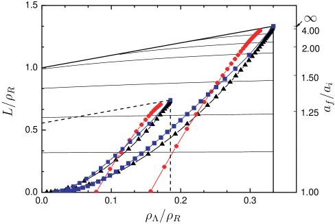
Fig. 1 shows the region in the -plane allowed by thermodynamics, and inside that, the contours of constant time . On the right axis we have indicated some values of (which depend only on ). The points correspond to some of the phase transitions considered in the next section. We have plotted two sets of curves, corresponding to and . The dashed line delimits the allowed region for the latter case. As the phase transition becomes stronger, the latent heat increases. However, the limit is reached for , together with the limit . That is why all the curves approach the upper-right corner of the allowed region.
The analytic approximation given by Eq. (14) for the total duration of the phase transition is valid only if condition (8) is satisfied. Furthermore, we cannot describe, within this approach, the transition between supercooling and phase coexistence, i.e., the reheating stage. A complete description of phase transition dynamics involves the computation of the nucleation rate. This requires specifying a model for the free energy.
III The free energy
We will consider a theory described by a scalar field with tree-level potential
| (17) |
which has a maximum at and a minimum at The one-loop effective potential is of the form
| (18) |
where is the one-loop zero-temperature correction, and we have added a constant so that the energy density vanishes in the true vacuum. Imposing the renormalization conditions that the minimum of the potential and the mass of do not change with respect to their tree-level values ah92 , the one-loop correction is given by
| (19) |
where is the number of d.o.f. of each particle species, is the -dependent mass, and the upper and lower signs correspond to bosons and fermions, respectively.
The free energy density results from adding finite-temperature corrections to the effective potential,
| (20) |
where the one-loop contribution is
| (21) |
and , stand for the contributions from bosons and fermions, respectively,
| (22) |
For simplicity, we will consider in general masses of the form , where is the Yukawa coupling. Thus, the free energy takes the form
| (23) | |||||
where the last term accounts for the contribution of species with , so is the effective number of d.o.f. of relativistic particles. The constant is obtained by imposing that , so
| (24) |
Notice that gives the energy density of the false vacuum,
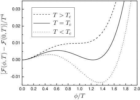
At high temperature the free energy (23) has a single minimum at . As the temperature decreases, a non-zero local minimum develops. Therefore, the free energy in the high- and low-temperature phases is given by and , respectively. In the phase with , all particles are massless and
| (25) |
where is the effective number of d.o.f. ( stands for bosons and for fermions). Thus we have radiation and false vacuum. At the critical temperature , the two minima and have the same free energy. Below this temperature, becomes the global minimum. In general, as temperature decreases further the barrier between minima disappears and the minimum at becomes a maximum. This happens at a temperature given by
| (26) |
Finally, at zero temperature we have , so . Notice, however, that the zero-temperature boson contribution may turn the maximum at of the tree-level potential into a minimum of . In this case, there will be two minima still at . Indeed, for , the r.h.s. of Eq. (26) becomes negative, which means that the barrier never disappears. Furthermore, for strongly coupled bosons the origin can become the stable zero-temperature minimum. Indeed, for the vacuum energy density (24) becomes negative. In that case, the origin is stable at all temperatures, and there is no phase transition.
The energy density can be derived from the free energy by means of the relations and . Thus, from Eq. (25) we obtain , and . At , , so the latent heat is . Taking into account that , we find
| (27) |
The functions are negative and monotonically increasing, so we see that the one-loop effective potential satisfies the thermodynamical bound . Furthermore, and fall exponentially for large . Therefore, approaches the limit for .
For our purposes it will be sufficient to consider only four particle species, namely, two bosons and two fermions. In this way we can have weakly coupled fermions and bosons with Yukawa couplings and , and d.o.f. and , respectively. These particles will be relatively light in the low-temperature phase. We will consider also bosons and fermions with variable couplings and , respectively. The values of the Yukawa couplings are constrained by perturbativity of the theory, which sets a generic upper bound cmqw05 . In addition, we include light d.o.f., for which we assume . This model allows us to explore several kinds of phase transitions.
For instance, choosing we have a phase transition at the electroweak scale. We obtain a good approximation for the free energy of the Standard Model (SM) if we consider fermion d.o.f. with (corresponding to the top), and boson d.o.f. with (corresponding to the transverse gauge vectors and ). The rest of the SM d.o.f. have , so their contribution to the -dependent part of the effective potential is negligible. They only contribute to in Eq. (23). To make the electroweak phase transition strongly first-order we need to add some extra particles to the SM. For our purposes, we don’t need to refer to any specific extension of the model. We choose , which corresponds to a Higgs mass , and we consider for the time being adding equal numbers of bosons and fermions, with and , which give a value for the minimum of the potential at the critical temperature (see Fig. 2).
It is well known that heavy bosons enhance the strength of the phase transition. We see in the left panel of Fig. 3 that the minimum , as well as the height of the barrier, increase if we increase the value of . Besides, the critical temperature decreases. Indeed, for fixed , according to Eq. (26) the temperature vanishes for a value given by . At this point, a barrier appears in the zero-temperature effective potential, and becomes a local minimum of . If is increased further, the zero-temperature barrier increases as the energy of the origin decreases. According to Eq. (24), the two zero-temperature minima become degenerate for a value given by . For this value of the critical temperature vanishes and . Beyond the value there is no phase transition.
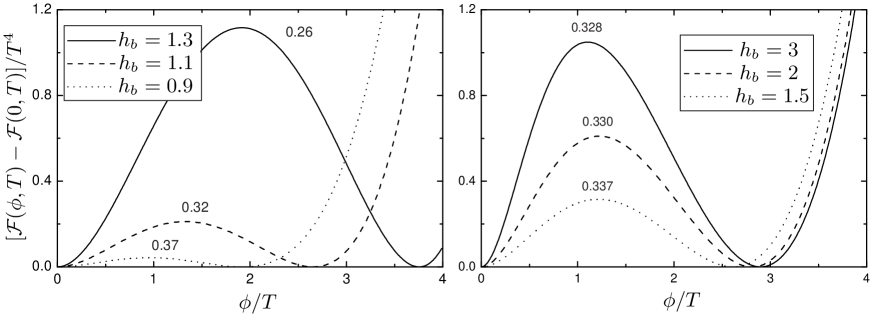
If we keep as we increase , the behavior is quite different, since the fermions compensate the effect of the bosons. As we can see in Fig. 3 (right panel), the height of the barrier increases more slowly with , and the value of does not change significantly. With this symmetric choice of parameters, the false vacuum energy density (24) does not depend on and . Thus, the origin will never be the stable minimum at , and will never vanish. According to Eq. (26), the temperature does not vanish either, but it decreases as . In the next section we will analyze the effect of these two opposite variations.
For large couplings, the first-order phase transition becomes stronger and the latent heat (27) increases. The maximum value will be achieved when all the couplings are large. If , this maximum becomes , with . Consider the case and . For fixed, the maximum is reached at , i.e., when . For the case we obtain the points in the -plane that are shown in blue squares in Fig. 1. For , on the contrary, there is no such limit on . In this case (black triangles in Fig. 1), as the coupling is increased the points accumulate near the point , which is the corner of the thermodynamically allowed region. In particular, for , we see that can be very close to the maximum , even though in this case does not vanish.
It is interesting to consider the case . Notice, however, that strong fermion couplings may destabilize the zero-temperature potential, since they introduce negative quartic terms in . To stabilize the potential in the case of a strongly coupled fermion, we can add a heavy boson with the same coupling and d.o.f. , and a mass cmqw05 . If is large enough, this boson will be decoupled from dynamics at . The maximum value of consistent with stability is obtained by requiring the quartic term to be positive for . It is given by
| (28) |
For a weakly-coupled fermion, is much larger than and the stabilizing boson is completely decoupled. On the contrary, for large , approaches and we recover the previous case. We have plotted in Fig. 1 the points of the -plane333The definitions of and change slightly in this case. corresponding to a variation of (red circles). For small values of we have only the fermion contribution, and the phase transition is weakly first-order. In fact, there is a minimum value of for which the phase transition becomes second-order. At this point, the latent heat vanishes for a finite value of . In contrast, for large we have, as in the previous cases, a strongly first-order phase transition.
As we see in Fig. 1, in all the cases the total duration of the phase transition becomes significant for large . However, the durations of supercooling and phase coexistence can be extremely different in each case.
IV The phase transition
IV.1 Phase transition dynamics
The nucleation and growth of bubbles in a first order phase transition has been extensively studied (see e.g. h95 ; qcd ; hkllm93 ; ah92 ; dlhll92 ; eikr92 ). According to the conventional picture of bubble nucleation, at the field takes the value throughout space. At , bubbles of the stable phase (i.e., with the value inside) nucleate. We remark that in a weakly first-order phase transition this picture may not work gkw91 . A quantitative determination of the importance of subcritical bubbles requires in general numerical calculations and is out of the scope of the present investigation. For instance, lattice calculations for the case of the minimal standard model (with unrealistically small values of the Higgs mass) show that subcritical bubbles may play a significant role at the onset of a weakly first-order electroweak phase transition yy97 . Thus, our results for the amount of supercooling become unreliable in the limit of very small values of the coupling .
The thermal tunneling probability for bubble nucleation per unit volume per unit time is a81 ; l83
| (29) |
The prefactor involves a determinant associated with the quantum fluctuations around the instanton solution. In general it cannot be evaluated analytically. However, the nucleation rate is dominated by the exponential in (29), so we will use the rough estimation . The exponent in Eq. (29) is the three-dimensional instanton action
| (30) |
where . The configuration of the nucleated bubble may be obtained by extremizing this action. It obeys the equation
| (31) |
Hence, coincides with the free energy that is needed to form a bubble in unstable equilibrium between expansion and contraction. At the critical temperature the bubble has infinite radius, so and In contrast, at the radius vanishes, so and , which is an extremely large rate in comparison to . Therefore, the number of bubbles will become appreciable at a temperature which is rather closer to than to . Thus, in order to have supercooling at , the temperature must not exist, so that the barrier between minima persists at .
After a bubble is formed, it grows due to the pressure difference at its surface. There is a negligibly short acceleration stage until the wall reaches a terminal velocity due to the viscosity of the plasma (see, e.g., m00 ). The velocity is determined by the equilibrium between the pressure difference and the force per unit area due to friction with the surrounding particles, . Thus,
| (32) |
The friction coefficient can be written as where is a dimensionless damping coefficient that depends on the viscosity of the medium, and is the bubble wall tension (for a review and a discussion see m04 ).
We will assume that the system remains close to equilibrium, which is correct if is small enough. If the wall velocity is lower than the speed of sound in the relativistic plasma, , the wall propagates as a deflagration front. This means that a shock front precedes the wall, with a velocity . For , the latent heat is transmitted away from the wall and quickly distributed throughout space. We can take into account this effect by considering a homogeneous reheating of the plasma during the expansion of bubbles h95 ; m01 . (For detailed treatments of hydrodynamics see, e.g., eikr92 ; hkllm93 ).
The radius of a bubble that nucleates at time and expands until time is
| (33) |
The scale factor takes into account the fact that the radius of a bubble increases due to the expansion of the Universe. The initial radius can be calculated by solving Eq. (31) for the bubble profile . It is roughly . Hence, can be neglected, since the second term in Eq. (33), which is determined by the dynamics, depends on the time scale
The fraction of volume occupied by bubbles is given by
| (34) |
The integral in the exponent gives the total volume of bubbles (in a unit volume) at time , ignoring overlapping. The complete expression (34) takes into account bubble overlapping gw81 . The factors of take into account that the number density of nucleated bubbles decreases due to the expansion of the Universe.
To integrate Eq. (34), we still need two equations in order to relate the variables , and . Eqs (5) and (7) give the relation m04
| (35) |
where the first term, which is proportional to the released entropy , accounts for reheating, and the second term accounts for the cooling of the Universe due to the adiabatic expansion. Finally, the Friedmann equation (12) gives the relation
| (36) |
with , where , and .
The functions and are easily obtained by numerically finding the minimum . The nucleation rate can be calculated by solving numerically Eq. (31) for the bubble profile, then integrating Eq. (30) for the bounce action, and using the result in Eq. (29). We solved Eq. (31) iteratively by the overshoot-undershoot method444We have checked our program by comparing with the results of Ref. dlhll92 for the bounce and Ref. ma05 for the evolution of the phase transition.. The thermal integrals (22) for the finite-temperature effective potential can be computed numerically. However, we find that the computation time is lowered significantly by using instead low- and high- expansions for (see the appendix).
IV.2 Numerical results
We begin by considering a phase transition at the electroweak scale, with the free energy plotted in Fig. 2. The development of the phase transition depends on the specific heat of the thermal bath, i.e., on the total number of d.o.f. We can take into account the light d.o.f. of the SM by setting in the last term of Eq. (23). The friction coefficient depends on the model and its computation is not straightforward. For the time being, let us assume . The solid curve in Fig. 4 shows the temperature variation during the phase transition for this model. We observe a considerable reheating, which indicates that the latent heat is comparable to the energy density needed to take the radiation back to . However, a phase coexistence stage is not achieved, which reveals that . Notice that the large number of d.o.f () makes the energy density of radiation much larger than the latent heat. For lower values of , the thermal bath has a smaller specific heat and is more easily reheated. This can be seen in the dashed and dashed-dotted lines in Fig. 4.
We note that supercooling finishes at a temperature which is quite closer to than to . As mentioned before, this fact is quite general, as it is due to the extremely rapid variation of the nucleation rate, which becomes at . Notice also that the different curves in Fig. 4 coincide during supercooling. This is because in this stage the relation between the dimensionless variables and is almost independent of any parameter of the model. Indeed, during supercooling , and the dependence of the scale factor on time is given by . Since and for , we have as long as does not depart significantly from .
We can check the approximation (14) for the total duration of the phase transition. The relevant parameters and are different for each curve in Fig. 4, since depends on . We obtain the time lengths , and . As expected, this approximation gives the correct value only when gets close to ; otherwise, Eq. (14) gives just a lower bound for .
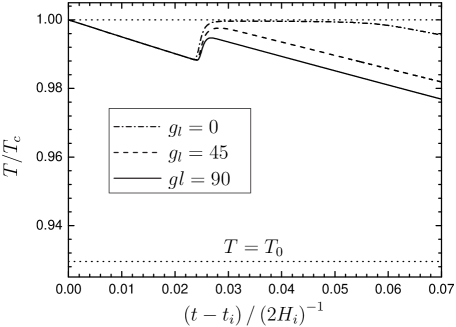
Fixing now an intermediate value (), which shows more clearly the effect of reheating, we consider three different values of the friction (solid curves in Fig. 5), in the range . These correspond to velocities which have values between and before reheating. We see that, as expected, reheating begins earlier for larger initial velocities. However, a variation of two orders of magnitude in does not change significantly the amounts of supercooling and reheating. For the rest of the paper, we will consider .

It is interesting to examine the role of the energy scale in the dynamics of the transition. The model of Eq. (23) has a single parameter with dimensions, namely, the minimum , since the masses of all the particles are of the form (notice that even the mass (28) of the stabilizing boson is proportional to ). Thus, dimensionless quantities such as e.g. the ratio will not be altered if we change the value of . This holds for all the quantities that are derived from the free energy (e.g., ), since the shape of the normalized effective potential in Fig. 2 is unaffected. Therefore, changing the scale will not affect the dynamics of the transition, except for the expansion rate of the Universe Eq. (36), which depends on the ratio .
To see the effect of such a change of scale, we have included in Fig. 5 a couple of examples in which the free energy is the same as before, apart from the value of . We considered the QCD scale, , and a scale , corresponding to a very recent phase transition (right and left dashed lines, respectively). Again, the temperature decreases at the same rate during supercooling, as explained above. However, bubble nucleation and reheating begin sooner. This happens because at later epochs the expansion rate is slower. As a consequence, the nucleation rate becomes with a smaller amount of supercooling. In contrast, has the same value for any scale . Thus, since is smaller, the temperature gets closer to . Hence, phase coexistence is favored in phase transitions occurring at later times. The parameters and have the same values for all the curves in Fig. 5, and Eq. (14) yields .
So far we have varied the parameters , , and , which do not change the shape of the effective potential. We shall now consider different values of the couplings and , fixing for simplicity . We have checked that fixing instead and and considering different values of and gives similar results. In what follows, we will set . The result is shown in Fig. 6. In the upper panels we plot the temperature reached during supercooling, together with the temperatures and . Notice that is always closer to than to . The lower panels show the time at which the temperature is reached, i.e., the duration of supercooling (solid line). The estimated duration of the phase transition is also shown, for different values of . As we increase the number of light particles (without changing the potential), we obtain less reheating for the same amount of supercooling. Hence, increasing gives the same but a lower .
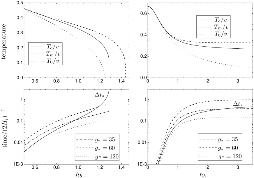
The left panels of Fig. 6 illustrate the effect of a variation of with fixed. As we have seen in the previous section, in this case the temperature vanishes for a value , where a zero-temperature barrier appears. For a value , the critical temperature also vanishes. The temperature lies between and , so it must vanish for some value with (in the present case, ). Our numerical calculation does not allow us to plot the curve of up to this limit, because the supercooling time diverges for . This can be seen in the lower left panel. For the system never gets out of the supercooling stage. On the contrary, for the phase transition completes in a finite time. Regarding phase coexistence, it occurs when . For a given , this happens up to a value of which is less than . Beyond that value, the supercooling temperature is too low for the latent heat to provide the required amount of reheating. Then, the estimation (14) for breaks down and the duration of the phase transition is just given by , since the phase coexistence stage is replaced by a short reheating (see e.g. Fig. 4).
If we now keep as we increase (right panels in Fig. 6), we see that does not vanish, and decreases like as expected. In this case, the supercooling time does not diverge at any finite value of , and can be considerably larger than . We see that for small values of there is phase coexistence for any value of . On the contrary, for large values of there is no phase coexistence at all, and the estimation for breaks down. The curves of saturate for large because, for , the parameters and cannot get close to their limits , .
Let us now consider the case in which , but the boson mass squared has a constant term given by Eq. (28) so it is partially decoupled from the thermodynamics. The curves we obtained are similar to those in the right panels of Fig. 6, except that the temperatures meet at a finite value . At this point the times fall to zero, since the phase transition becomes second-order. We have plotted in Fig. 7 the ratio for this case and those of Fig. 6. For each set of curves, the supercooling fraction increases with , since decreases. We also see that phase coexistence is favored for . This is because fermions contribute to the latent heat without enhancing the strength of the transition.

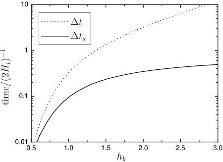
In general, the energy density of radiation, , is much larger than the latent heat, since only strongly coupled particles contribute significantly to the latter. It is interesting to consider the case in which there are no light d.o.f. at all, i.e., . Only in this case the parameters can be close to the thermodynamical limits , . In the absence of light particles, all the latent heat that is released during bubble expansion is absorbed only by the heavy particles, which are thus more easily reheated. Consequently, this scenario will be the most favorable for phase coexistence. We plot the time intervals in Fig. 8 for the case . We find, as expected, that the phase coexistence time is notably enhanced. For lower scales we will have the same but a smaller .
V Phase transition dynamics and Cosmology
The cosmological implications of a phase transition depend drastically on the dynamics. In this section we discuss how the different steps in the evolution, namely, supercooling, reheating and phase coexistence, affect some of the observable products of a phase transition.
V.1 Late-time phase transitions and false vacuum energy
Late-time phase transitions have been studied in connection to the formation of large-scale structure and have been related, for instance, to axions, domain walls and neutrino masses (see e.g. fhw92 ). In contrast to those occurring in the early Universe, which take place in the presence of a hot plasma with a large number of degrees of freedom, low-scale phase transitions happen in general in a sector with a few d.o.f. and, consequently, a small specific heat. Therefore, one expects a significant reheating during the phase transition, and a long phase coexistence stage m06 . Indeed, we have seen in section IV that both a low and a small favor a long phase coexistence period (see e.g. Figs 4 and 5). This stage can be significantly long for strongly first-order phase transitions, as shown in Fig. 6 (lower right panel). In particular, if all the particles have strong couplings, Fig. 8 shows that the coexistence of phases can last for a time .
Recently, late-time phase transitions have been considered with the aim of (partially) solving the dark-energy problem. While the system is trapped in the metastable phase, the energy density of the false vacuum provides an effective cosmological constant. Thus, a false vacuum energy could explain the observed acceleration of the Universe. This fact has motivated several models in which a phase transition at a scale occurs in a hidden sector darke ; m06 ; g00 ; chn04 . Such a false vacuum must persist until the present epoch. Hence, since the temperature of the hidden sector must be lower than that of photons, , the system must be in the metastable phase still at (for a discussion, see e.g., m06 ; g00 ). This could be achieved, in principle, in several ways, namely, due to a low critical temperature chn04 , due to a large amount of supercooling g00 , or due to a long phase coexistence stage m06 .
The constraint on the temperature of the hidden sector, , comes from the Big Bang Nucleosynthesis (BBN) constraint on its radiation energy density, . Therefore, if the false vacuum energy is to explain the observed dark energy, the temperature of the system must be such that
| (37) |
One possible way out of this limitation would be to assume that, although the BBN constraint was satisfied for most of the history of the Universe, when reached the system entered a long phase coexistence stage at constant temperature m06 . Then, as continued decreasing, the temperature of the hidden sector was stuck at . Thus, the BBN condition would be violated only at the present epoch, avoiding the restriction (37). As we have seen in section II, a very long phase coexistence stage is possible. However, the effective cosmological constant during phase coexistence is which, according to the thermodynamical bound Eq. (15), is negative and does not lead to accelerated expansion.
Due to the bound , the condition (37) cannot be fulfilled at . This automatically rules out any model in which false vacuum energy is dominant because the phase transition is yet to occur. For instance, in Ref. chn04 a potential with a negative quadratic term is considered. In that model, the temperature is assumed to be high enough that thermal corrections trap the system in the false vacuum. Then, the condition (37) is shown to be achieved for a somewhat small value of a coupling constant . Clearly the thermodynamical bound is strongly violated. However, the thermal correction to the effective potential is assumed to be , which corresponds to keeping only the quadratic term in the power expansion of the thermal integral . It is then argued that the field is trapped at the origin as long as is large enough to cancel the negative mass squared. This would be correct in a second-order phase transition, in which . However, with the parameters of Ref. chn04 the phase transition is strongly first-order. Hence, at the field certainly lies in the minimum . The critical temperature can in fact be much larger than , as shown in the upper-left panel of Fig. 6, where we see that can vanish while is still of order .
Another possibility to attain condition (37) is in a model with a large amount of supercooling, so that but . This is possible in a strongly first-order phase transition. For the model considered in the left panel of Fig. 6, there is a maximum value of the coupling for which the supercooling temperature and the duration of supercooling becomes infinite. It is not clear, however, that the required amount of supercooling can be achieved in a realistic model. Notice that, even when vanishes (i.e., for ), we still have . In the example of Fig. 6, . Thus, it is necessary to go beyond , i.e., to consider a model which has a barrier still at . In Ref. g00 the condition (37) was accomplished in a specific model with and some fine tuning of the parameters. However, the thermal corrections were taken into account only by introducing a term . As pointed out in Ref. m06 , this causes an unrealistically large value of the latent heat, which violates the constraint Eq. (16).
V.2 Electroweak baryogenesis and baryon inhomogeneities
It is well known that the electroweak phase transition could be the framework for the generation of the baryon number asymmetry of the Universe (BAU). A first-order electroweak phase transition provides the three Sakharov’s conditions for the generation of a BAU, although physics beyond the minimal Standard Model is mandatory in order to obtain a quantitatively satisfactory result ckn93 . Due to violating interactions of particles with the bubble walls, a net baryon number density is generated around the walls of expanding bubbles. Assuming that violation is strong enough and that the baryon number violating sphaleron processes are suppressed in the broken symmetry phase, the resulting depends on the bubble wall velocity . If the velocity is too large, sphalerons will not have enough time to produce baryons. On the other hand, for very small velocities thermal equilibrium is restored and sphalerons erase any generated baryon asymmetry. As a consequence, the generated baryon number has a peak at a given wall velocity, which is generally lmt92 ; ckn92 ; ck00 .
As we have seen, reheating is always appreciable, even if there is no phase coexistence555An exception could be the case of an extremely supercooled electroweak phase transition, for which reheating may be negligible. Such a model has been considered recently in Ref. nqw07 .. The temperature rise causes the wall velocity to descend significantly. Thus, baryogenesis is either enhanced or suppressed, depending on which side of the peak of the initial velocity lies h95 ; m01 . Furthermore, baryon inhomogeneities arise due to the variation of . Electroweak baryon inhomogeneities may survive until the QCD scale s03 ; jf94 and affect the dynamics of the quark-hadron phase transition s03 ; cm96 ; h83 . The geometry of the inhomogeneities was studied in Refs. ma05 ; h95 . Since baryon number is generated near the bubble walls, a spherical inhomogeneity with a radial profile is formed inside each expanding bubble.
Notice that bubble nucleation stops as soon as reheating begins. In fact, due to the exponential variation of the nucleation rate with temperature, most bubbles are formed in a small interval around the time at which the minimum temperature is reached ma05 . This interval is in general much shorter than the time it takes expanding bubbles to complete the phase transition. Therefore, it is a good approximation to assume that all bubbles are created at . At a later time, their walls are moving with a velocity . Hence, all the inhomogeneities have the same profile.
In Refs. ma05 ; h95 , the size and amplitude of the electroweak baryon inhomogeneities were investigated using a simple effective potential, whose parameters were adjusted so as to give the desired values of the thermodynamic parameters. This approximation allows to vary independently parameters such as, e.g., the latent heat or the bubble-wall tension. These parameters, though, are generally related in a non-trivial way, which depends on the extension of the SM that is considered. For instance, a strongly first-order phase transition will have in general a considerable amount of supercooling, and also a large latent heat. However, the relative importance of supercooling and reheating depends significantly on the specific model, as can be seen, for instance, in Fig. 7.
The amplitude of the baryon inhomogeneities, , is bounded by the ratio of the highest and lowest wall velocities reached during bubble expansion, . If is freely varied, one can achieve values or higher ma05 ; h95 . However, in a specific extension of the SM this will not be necessarily so. To examine a more realistic situation, we have considered extensions of the SM as in the previous sections. We find that, if we add a strongly coupled boson, or a boson and a fermion with , the velocity variation is in general . We find a sizeable ratio only in the case in which the fermion dominates. The addition of strongly coupled fermions was investigated in Ref. cmqw05 , in order to make the electroweak phase transition strongly first-order.
Let us consider for simplicity an extension with fermionic d.o.f. with mass , and stabilizing bosons with , , and a dispersion relation , with given by Eq. (28). We obtain the plot of Fig. 9. For in the range of the figure the value of the order parameter is , as required by electroweak baryogenesis.

The distance scale of the inhomogeneities is given by the final size of bubbles, which depends on the distance between centers of nucleation. Thus, it can be roughly estimated as . For the present case we obtain the dashed-dotted curve in Fig. 10. Our results for the distance agree in order of magnitude with those of Refs. ma05 ; h95 . However, we see that the amplitude of the inhomogeneities can be important only for small values of . In particular, is reached for values of for which . Therefore, baryon inhomogeneities of significant amplitude are not likely produced in the electroweak phase transition.

V.3 Topological defects and magnetic fields
If a global symmetry is spontaneously broken at a first-order phase transition, the phase angle of the Higgs field takes different and uncorrelated values inside each nucleated bubble. When bubbles collide, the variation of the phase from one domain to another is smoothed out. According to the geodesic rule, the shortest path between the two phases is chosen k76 . When three bubbles meet, a vortex (in two spatial dimensions) or a string (in 3d) may be trapped between them. This mechanism can be generalized to higher symmetry groups and other kinds of topological defects.
If the dynamics for the phase is not taken into account, the number density of defects depends only on the final bubble size. The probability of trapping a string at the meeting point of three bubbles is . Thus, the string density (length per unit volume) is , where is the distance between bubble centers kv95 . Fig. 10 shows the different possibilities for the length . For stronger phase transitions, the bubble separation is larger, since the nucleation rate is more suppressed.
Taking into account the dynamics of phase equilibration, the number density of defects depends also on the velocity of bubble expansion. If the latter is much less than the velocity of light, the equilibration between the phases of two bubbles may complete before a third bubble meets them, thus reducing the chances of trapping a string. Consequently, reheating hinders the formation of topological defects.
In the case of a gauge theory, a spatial variation of the phase is linked to a variation of the gauge field kv95 . As a consequence, a magnetic field is generated together with the phase difference in the collision of two bubbles. Then, one can say that a vortex is formed whenever a quantum of magnetic flux is trapped in the unbroken-symmetry region between three bubbles. The phase equilibration process is thus related to flux spreading, and depends on the conductivity of the plasma. Bubble collision constitutes also a mechanism for generating the cosmic magnetic fields (see e.g. gr98 ). This mechanism may take place at the electroweak phase transition, where unstable cosmic strings and hypermagnetic fields may be formed. The latter are subsequently converted to magnetic fields.
A detailed calculation of the density of defects and the magnitude of the magnetic fields is beyond the scope of this paper and we leave it for future research. Although some simulations have been made (see, e.g., bkvv95 ), several simplifications are generally used, which include assuming a constant nucleation rate and a constant bubble wall velocity. As we have seen, this situation is hardly realistic. Moreover, the formation of topological defects and magnetic fields depend strongly on the dynamics of the phase transition. In particular, a long phase coexistence stage with a very slow bubble expansion will affect significantly the mechanism of phase equilibration during bubble percolation.
VI Conclusions
In this article we have investigated the different stages in the development of first-order phase transitions of the Universe. In particular, we have studied the amounts of supercooling and reheating. If the entropy discontinuity is larger than the entropy decrease during supercooling, a phase-coexistence stage is reached. Then, the total duration of the phase transition can be calculated analytically. The ratio depends only on the parameters and . If , supercooling lasts for a time which is longer than . In this case, there is no phase coexistence, and gives only a lower bound for the total duration of the phase transition. We have shown that thermodynamics constrain these parameters to the region , . These constraints should be taken into account when the dynamics of a particular phase transition is considered, since approximations for the effective potential may violate them, and thus the analysis may lead to incorrect results.
With the help of a simple model, we have analyzed numerically the role of different parameters in the dynamics of the phase transition. We have verified that phase coexistence is more likely in later phase transitions, since both a lower energy scale and a smaller number of degrees of freedom favor reheating. In addition, we have seen that changing the viscosity of the surrounding medium does not affect significantly the dynamics of supercooling and reheating, although it affects the velocity of bubble walls. The incorporation of bosons to a given model strengthens the phase transition, so the effect on the dynamics is to enlarge the latent heat and suppress the nucleation rate. As we have seen, the latter effect is in general stronger, so adding bosons favors supercooling. On the contrary, adding fermions in general weakens the phase transition and at the same time increases the number of d.o.f. We have checked that in this case phase coexistence is favored.
We have studied how our general results on phase transition dynamics may affect some of the cosmological consequences. For instance, in the case of dark energy from a phase transition, we have shown that the thermodynamical bounds rule out some models. Besides, we have analyzed the effect of dynamics on two important parameters, namely, the number density of bubbles and the amplitude of the velocity variation during reheating. As we have seen, these quantities are relevant for the generation of different cosmological relics, e.g., baryon inhomogeneities, topological defects and magnetic fields. In particular, we have found that it is difficult to obtain baryon inhomogeneities of sizeable amplitude in realistic models of the electroweak phase transition.
We believe that our results on the dynamics can be applied to a wide class of phase transitions of the Universe, and the discussion on the cosmological consequences can be extended to several interesting possibilities, such as, e.g., the formation of baryon inhomogeneities in the quark-hadron phase transition w84 or the generation of gravitational waves gs07 .
Acknowledgements.
This work was supported in part by Universidad Nacional de Mar del Plata, Argentina, grants EXA 338/06 and 365/07. The work by A.D.S. was supported by CONICET through project PIP 5072. The work by A.M. was supported by FONCyT grant PICT 33635.Appendix A Approximations for the thermal integrals
In this appendix we consider expansions of the functions for small and large . The integrals in Eq. (22) can be evaluated numerically. However, a numerical computation in the effective potential increases significantly the total computation time. Indeed, notice that for each temperature, we must find the minimum to compute several quantities derived from . Moreover, the calculation of the bounce action requires the time-demanding overshoot-undershoot technique to solve Eq. (31) for the bubble profile at each . Therefore, it is useful to employ analytical approximations for the thermal integrals.
Following the derivation of Ref. dj74 , we can obtain the expansions of in powers of For bosons we have
where is given by with the Euler constant; is the Riemann zeta function, and is the Gamma function. The expansion for fermions is
where is given by . For any value of we can get the desired precision by keeping enough terms in these expansions. For example, keeping up to in and in we obtain a precision of for .
The expansion for large can be obtained by changing the variable of integration to and expanding the logarithm in Eq. (22) in powers of (see Ref. ah92 ),
| (40) |
For each the integral yields , where is the modified Bessel function of the second kind abramowitz . Hence, we obtain the expansions
| (41) |
Notice that the integrals in Eq. (40) are of the order of , so the terms in this expansion decrease with powers of . Therefore, in general we will obtain the desired precision by considering a few terms. For example, for we obtain by keeping only the first two terms in (41). For , keeping terms up to in the expansion gives a precision . As a rough estimation of the error of the truncated expansion, we note that the -th term is and the error is given by the ratio of the -th term to the first term, .
References
- (1) For a review, see A. Vilenkin and E.P.S. Shellard, Cosmic Strings and Other Topological Defects (Cambridge University Press, Cambridge, England, 1994).
- (2) D. Grasso and H. R. Rubinstein, Phys. Rept. 348, 163 (2001) [arXiv:astro-ph/0009061].
- (3) For reviews, see A. G. Cohen, D. B. Kaplan and A. E. Nelson, Ann. Rev. Nucl. Part. Sci. 43, 27 (1993) [arXiv:hep-ph/9302210]; A. Riotto and M. Trodden, Ann. Rev. Nucl. Part. Sci. 49, 35 (1999) [arXiv:hep-ph/9901362].
- (4) A. F. Heckler, Phys. Rev. D 51, 405 (1995) [arXiv:astro-ph/9407064].
- (5) E. Witten, Phys. Rev. D 30, 272 (1984).
- (6) See, e.g., C. Grojean and G. Servant, Phys. Rev. D 75, 043507 (2007) [arXiv:hep-ph/0607107], and references therein.
- (7) S. G. Rubin, M. Y. Khlopov and A. S. Sakharov, Grav. Cosmol. S6, 51 (2000) [arXiv:hep-ph/0005271]; R. V. Konoplich, S. G. Rubin, A. S. Sakharov and M. Y. Khlopov, Phys. Atom. Nucl. 62, 1593 (1999) [Yad. Fiz. 62, 1705 (1999)].
- (8) J. A. Frieman, C. T. Hill, A. Stebbins and I. Waga, Phys. Rev. Lett. 75, 2077 (1995); J. A. Frieman, C. T. Hill and R. Watkins, Phys. Rev. D 46, 1226 (1992); A. Singh, Phys. Rev. D 52, 6700 (1995) [arXiv:hep-ph/9412240].
- (9) A. Megevand, Phys. Lett. B 642, 287 (2006) [arXiv:astro-ph/0509291].
- (10) Z. Chacko, L. J. Hall and Y. Nomura, JCAP 0410, 011 (2004).
- (11) H. Goldberg, Phys. Lett. B 492, 153 (2000).
- (12) P. J. Steinhardt, Nucl. Phys. B 190, 583 (1981); D. Spector, Phys. Lett. B 194, 103 (1987); A. Kusenko, Phys. Lett. B 406, 26 (1997) [arXiv:hep-ph/9705361]; D. Metaxas, Phys. Rev. D 63, 083507 (2001) [arXiv:hep-ph/0009225].
- (13) M. Gleiser, E. W. Kolb and R. Watkins, Nucl. Phys. B 364, 411 (1991).
- (14) A. Mégevand, Phys. Rev. D 69, 103521 (2004) [arXiv:hep-ph/0312305].
- (15) E. Suhonen, Phys. Lett. B 119, 81 (1982).
- (16) K. i. Iso, H. Kodama and K. Sato, Phys. Lett. B 169, 337 (1986).
- (17) K. Sato, Mon. Not. Roy. Astron. Soc. 195, 467 (1981).
- (18) G. W. Anderson and L. J. Hall, Phys. Rev. D 45, 2685 (1992).
- (19) M. Carena, A. Mégevand, M. Quiros and C. E. M. Wagner, Nucl. Phys. B 716, 319 (2005).
- (20) K. Enqvist, J. Ignatius, K. Kajantie and K. Rummukainen, Phys. Rev. D 45, 3415 (1992).
- (21) P. Y. Huet, K. Kajantie, R. G. Leigh, B. H. Liu and L. D. McLerran, Phys. Rev. D 48, 2477 (1993) [arXiv:hep-ph/9212224]; J. Ignatius, K. Kajantie, H. Kurki-Suonio and M. Laine, Phys. Rev. D 49, 3854 (1994) [arXiv:astro-ph/9309059]; H. Kurki-Suonio and M. Laine, Phys. Rev. D 51, 5431 (1995) [arXiv:hep-ph/9501216].
- (22) M. Dine, R. G. Leigh, P. Y. Huet, A. D. Linde and D. A. Linde, Phys. Rev. D 46, 550 (1992) [arXiv:hep-ph/9203203].
- (23) A. Mégevand and F. Astorga, Phys. Rev. D 71, 023502 (2005).
- (24) C. J. Hogan, Phys. Lett. B 133, 172 (1983); T. DeGrand and K. Kajantie, Phys. Lett. B 147, 273 (1984); K. Kajantie and H. Kurki-Suonio, Phys. Rev. D 34, 1719 (1986); D. Chandra and A. Goyal, Phys. Rev. D 62, 063505 (2000) [arXiv:hep-ph/9903466].
- (25) M. Yamaguchi and J. Yokoyama, Nucl. Phys. B 523, 363 (1998) [arXiv:hep-ph/9805333]; Phys. Rev. D 56, 4544 (1997) [arXiv:hep-ph/9707502].
- (26) I. Affleck, Phys. Rev. Lett. 46, 388 (1981).
- (27) A. D. Linde, Nucl. Phys. B 216, 421 (1983) [Erratum-ibid. B 223, 544 (1983)]; Phys. Lett. B 100, 37 (1981).
- (28) A. Megevand, Int. J. Mod. Phys. D 9, 733 (2000) [arXiv:hep-ph/0006177].
- (29) A. Mégevand, Phys. Rev. D 64, 027303 (2001) [arXiv:hep-ph/0011019].
- (30) A. H. Guth and E. J. Weinberg, Phys. Rev. D 23, 876 (1981).
- (31) W. D. Garretson and E. D. Carlson, Phys. Lett. B 315, 232 (1993); S. M. Barr and D. Seckel, Phys. Rev. D 64, 123513 (2001); J. Yokoyama, Phys. Rev. Lett. 88, 151302 (2002); N. Arkani-Hamed, L. J. Hall, C. F. Kolda and H. Murayama, Phys. Rev. Lett. 85, 4434 (2000).
- (32) B. H. Liu, L. D. McLerran and N. Turok, Phys. Rev. D 46, 2668 (1992); N. Turok, Phys. Rev. Lett. 68, 1803 (1992).
- (33) A. E. Nelson, D. B. Kaplan and A. G. Cohen, Nucl. Phys. B 373, 453 (1992).
- (34) J. M. Cline and K. Kainulainen, Phys. Rev. Lett. 85, 5519 (2000) [arXiv:hep-ph/0002272]; J. M. Cline, M. Joyce and K. Kainulainen, JHEP 0007, 018 (2000) [arXiv:hep-ph/0006119]; M. Carena, J. M. Moreno, M. Quiros, M. Seco and C. E. Wagner, Nucl. Phys. B 599, 158 (2001) [arXiv:hep-ph/0011055].
- (35) G. Nardini, M. Quiros and A. Wulzer, JHEP 0709, 077 (2007) [arXiv:0706.3388 [hep-ph]].
- (36) S. Sanyal, Phys. Rev. D 67, 074009 (2003) [arXiv:hep-ph/0211208].
- (37) M. B. Christiansen and J. Madsen, Phys. Rev. D 53, 5446 (1996) [arXiv:astro-ph/9602071].
- (38) Y. Hosotani, Phys. Rev. D 27, 789 (1983).
- (39) K. Jedamzik and G. M. Fuller, Astrophys. J. 423, 33 (1994) [arXiv:astro-ph/9312063].
- (40) T. W. B. Kibble, J. Phys. A 9, 1387 (1976).
- (41) T. W. B. Kibble and A. Vilenkin, Phys. Rev. D 52, 679 (1995) [arXiv:hep-ph/9501266].
- (42) J. Ahonen and K. Enqvist, Phys. Rev. D 57, 664 (1998) [arXiv:hep-ph/9704334]; D. Grasso and A. Riotto, Phys. Lett. B 418, 258 (1998) [arXiv:hep-ph/9707265]; E. J. Copeland, P. M. Saffin and O. Tornkvist, Phys. Rev. D 61, 105005 (2000) [arXiv:hep-ph/9907437].
- (43) J. Borrill, T. W. B. Kibble, T. Vachaspati and A. Vilenkin, Phys. Rev. D 52, 1934 (1995) [arXiv:hep-ph/9503223]; M. Lilley and A. Ferrera, Phys. Rev. D 64, 023520 (2001) [arXiv:hep-ph/0102035].
- (44) L. Dolan and R. Jackiw, Phys. Rev. D 9, 3320 (1974).
- (45) M. Abramowitz and I. A. Stegun, Handbook of Mathematical Functions (Dover, New York, 1972).