The Numerical Simulation of Turbulence

Turbulence is a remarkable subject in physics. The underlying equations, which are in their simplest formulation the Euler equations, were published 250 years ago [20]. Yet a theoretical grasp of the phenomenology emerging from these equations had not been achieved before the mid-twentieth century, when Heisenberg [25] and Kolmogorov [33] obtain first analytical results. Eventually, it took the capabilities of modern supercomputers to obtain a full appreciation of the complexity that is inherent to the Euler equations. Astrophysics is now at the very frontier of numerical turbulence modelling. Among the additional ingredients for making turbulence in astrophysics even more complex are supersonic flow, self-gravity, magnetic fields and radiation transport. In contrast, terrestrial turbulence is mostly incompressible or only weakly compressive. External gravity is, of course, an issue in the computation of atmospheric processes on Earth. Self-gravity, however, is only encountered on large, astrophysical scales. The dynamics of turbulent plasma has met vivid attention in research related to nuclear fusion reactors but, otherwise, is not encountered under terrestrial conditions.

In this Chapter, I give an overview of the various approaches toward the numerical modelling of turbulence, particularly, in the interstellar medium (ISM). The discussion is placed in a physical context, i. e. computational problems are motivate from basic physical considerations. Presenting selected examples for solutions to these problems, I introduce the basic ideas of the most commonly used numerical methods. For detailed methodological accounts, the reader is invited to follow the references. Some important results and astrophysical implications are briefly outlined. Since turbulence, in a strict sense, is genuinely three-dimensional, I almost exclusively consider three-dimensional simulations. Furthermore, turbulence is a multi-scale phenomenon and, in order to capture its properties correctly, sufficient numerical resolution is essential. This is why newer higher-resolution computations are generally preferred as examples (as regards self-gravitating turbulence, however, high-resolution simulations are appearing just now and are not included here).

To begin with, I briefly discuss the equations which are numerically solved in astrophysics and related theoretical aspects. The following Sections deal with supersonic turbulence, self-gravitating turbulence and magnetohydrodynamic turbulence. Naturally, there are intersections. Representative examples for numerical simulations are placed depending on their main objectives. Finally, I give a resume of what has been achieved and which challenges are likely to be met.

1 Fundamentals

In the following, we consider self-gravitating inviscid fluid subject to the action of external force fields and, possibly, magnetic fields. The evolution of the mass density $\rho$, the velocity $v$ and the specific energy $e$ of the fluid is given by the compressible Euler equations:

$$\frac{\mathrm{D}}{\mathrm{D}t}\rho=-\rho\boldsymbol{\nabla}\boldsymbol{v},$$ (1)

$$\rho \frac{\mathrm{D}}{\mathrm{D}t}\boldsymbol{v}=-\boldsymbol{\nabla}P+\rho(\boldsymbol{f}+\boldsymbol{g}),$$ (2)

$$\rho \frac{\mathrm{D}}{\mathrm{D}t}e+\boldsymbol{\nabla}\cdot\boldsymbol{v}P=\Gamma-\Lambda+\rho\boldsymbol{v}\cdot(\boldsymbol{f}+\boldsymbol{g}),$$ (3)

where the Lagrangian time derivative is defined by

$$\frac{\mathrm{D}}{\mathrm{D}t}=\frac{\partial}{\partial t}+\boldsymbol{v}\cdot\boldsymbol{\nabla}.$$ (4)

The total energy per unit mass is given by

$$e=\frac{1}{2}v^{2}+\frac{P}{(\gamma-1)\rho},$$ (5)

where $\gamma$ is the adiabatic exponent and the pressure $P$ is related to the mass density and the temperature $T$ via the ideal gas law:

$$P=\frac{\rho k_{\mathrm{B}}T}{\mu m_{\mathrm{H}}}.$$ (6)

The constants $k_{\mathrm{B}}$, $\mu$ and $m_{\mathrm{H}}$ denote, respectively, the Boltzmann constant, the mean molecular weight and the mass of the hydrogen atom. The energy budget can be altered by heating ($\Gamma$) and cooling ($\Lambda$), by non-gravitational forces ($\rho f$) as well as gravity ($\rho g$). Generally, heating and cooling processes are important for the dynamics of the interstellar medium (Sections 3 & 4).

Non-gravitational forces supplying energy to the flow can be mechanical or magnetic. An example of a mechanical force would be the random driving force that is commonly used in turbulence simulations. This is an external force, i. e., it is independent of the dynamics of the fluid (Section 2). Quite the opposite holds for conducting fluids in the presence of magnetic fields. In the case of ideal magnetohydrodynamics, the fluid is dragged by the Lorentz force $\rho\boldsymbol{f}=\boldsymbol{J}\times\boldsymbol{B}$, where the current $\boldsymbol{J}=\boldsymbol{\nabla}\times\boldsymbol{B}$. The magnetic field $\boldsymbol{B}$, in turn, depends on the flow via Faraday’s law,

$$\frac{\partial\boldsymbol{B}}{\partial t}=\boldsymbol{\nabla}\times(\boldsymbol{v}\times\boldsymbol{B}).$$ (7)

The interaction between turbulent flow and magnetic fields alters properties of turbulence such as the scaling behaviour (Section 4).

The gravitational acceleration $\boldsymbol{g}=-\nabla\cdot\phi$ arises, in part, from the self-gravity of the fluid and, depending on the boundary conditions, the gravitational field of external sources. In the case of periodic boundary conditions, gravity is solely produced by density fluctuations with respect to the global mean (Section 3). In this case, the gravitational potential is determined by the Poisson equation

$$\nabla^{2}\phi=4\pi G(\rho-\langle\rho\rangle),$$ (8)

where $G$ is Newton’s constant. The mean mass density $\langle\rho\rangle=\rho_{0}$ is a constant because of mass conservation.

Letting the curl operator $\boldsymbol{\nabla}\times$ act upon equation (2), an evolutionary equation for the vorticity of the flow, $\omega=\boldsymbol{\nabla}\times\boldsymbol{v}$, is obtained:

$$\frac{\mathrm{D}}{\mathrm{D}t}\boldsymbol{\omega}=\boldsymbol{\mathsf{S}}\cdot\boldsymbol{\omega}-d\boldsymbol{\omega}+\frac{1}{\rho^{2}}\boldsymbol{\nabla}\rho\times\boldsymbol{\nabla}P+\boldsymbol{\nabla}\times\boldsymbol{f}.$$ (9)

The rate-of-strain tensor $\boldsymbol{\mathsf{S}}$ is the symmetrised velocity gradient and the divergence $d=\boldsymbol{\nabla}\cdot\boldsymbol{v}$. Apart from the stirring of fluid due to rotational force components, vorticity can be generated by the baroclinic term $\boldsymbol{\nabla}\rho\times\boldsymbol{\nabla}P$, if the gradient of the mass density and the pressure gradient are not aligned. With the ideal gas equation 6, it follows that baroclinic vorticity generation occurs in non-isothermal gas. The term $\boldsymbol{\mathsf{S}}\cdot\boldsymbol{\omega}-d\boldsymbol{\omega}$ accounts for the stretching of vortices caused by strain in addition to the expansion or contraction of vortices due to the compressibility of the fluid.

The time evolution of the divergence $d$ is given by

$$\begin{split}\frac{\mathrm{D}}{\mathrm{D}t}d=&\frac{1}{2}\left(\omega^{2}-|S|^{2}\right)-\frac{1}{\rho}\nabla^{2}P\\ &+\frac{1}{\rho^{2}}\boldsymbol{\nabla}\rho\cdot\boldsymbol{\nabla}P-4\pi G(\rho-\rho_{0})+\boldsymbol{\nabla}\cdot\boldsymbol{f}.\end{split}$$ (10)

This equation also follows from the conservation law (2) by applying the operator $\boldsymbol{\nabla}\cdot$ and substituting the Poisson equation for the gravitational potential (8). The norm of the rate of strain is defined by $|S|=(2S_{ij}S_{ij})^{1/2}$. From the first term, one can see that vorticity contributes to positive divergence, while strain is associated with negative divergence, i. e. converging flow. In the incompressible case, the first term on the right hand side of equation (10) is cancelled by the Laplacian of the pressure divided by the density. Whereas vorticity cannot be generated by a gradient field such as gravity, an increasing rate of convergence will be caused by gravity, if the term $4\pi G(\rho-\rho_{0})$ dominates. In this case, gravitational collapse of the gas ensues.

The numerical simulation of astrophysical turbulence has to account for all fluid dynamical processes which become manifest in the evolutionary equations of the vorticity (9) and the divergence (10). In many terrestrial applications, on the other hand, incompressible turbulence without gravity and magnetic fields is considered. Then equations (9) and (10) reduce to

$$\frac{\mathrm{D}}{\mathrm{D}t}\boldsymbol{\omega}=\boldsymbol{\mathsf{S}}\cdot\boldsymbol{\omega}+\boldsymbol{\nabla}\times\boldsymbol{f},$$ (11)

$$\frac{\mathrm{D}}{\mathrm{D}t}d=0.$$ (12)

The only possibility of generating vorticity in this case is to stir the fluid by solenoidal (rotational) forces. Non-linear turbulent interactions stretch and fold the large-scale eddies produced by stirring into thin vortex filaments. This is the very essence of turbulent fluid dynamics. Here, the question arises whether the generation of turbulence in the ISM resembles the scheme of stirring, stretching and folding at all. Interestingly, this presumption underlies the application of solenoidal driving forces in most numerical simulations.

Incompressible fluid dynamics serves as an important reference case for which scaling properties of isotropic turbulence in the ensemble average can be derived analytically. Kolmogorov [33] showed that the root mean square velocity fluctuations $v^{\prime}(\ell)$ at a certain length scale $\ell$ obey the so called $2/3$-law,

$$v^{\prime}(\ell)^{2}\propto\ell^{2/3},$$ (13)

provided that $\ell$ is small compared to the integral length scales $L$ at which energy is supplied to the flow. The 2/3-law implies that the rate of kinetic energy dissipation $\epsilon$ is asymptotically constant, as $\epsilon\sim v^{\prime}(\ell)^{3}/\ell\simeq\mathrm{const.}$ in the limit $\ell/L\ll 1$. This result is known as the law of positive energy dissipation [22]. Both the $2/3$ law and the law of positive energy dissipation appear to be robust properties of turbulence as long as the flow becomes isotropic and nearly incompressible towards small length scales. This is not always the case. Magnetic fields, for instance, introduce small-scale anisotropy. Moreover, there is no consensus yet to what extent the scaling properties of incompressible turbulence carry over to supersonic flow.

2 Supersonic turbulence

Turbulence is called supersonic, if the root mean square (RMS) Mach number $\mathcal{M}_{\mathrm{rms}}=\langle(v/c_{\mathrm{s}})^{2}\rangle^{1/2}$ exceeds unity. Kinetic energy dissipation in supersonic turbulence caused by shock fronts propagating through the fluid dominates viscous dissipation. Since the resulting dissipative heating rises the speed of sound to a value comparable to the typical flow velocity within a dynamical time, supersonic turbulence cannot be maintained, if the excess heat is not efficiently removed from the fluid. As an idealisation, heating is exactly balanced by cooling such that the temperature remains constant. In this case, continuously driven turbulent flow settles into a steady state in which the RMS Mach number is asymptotically constant. In isothermal gas, solenoidal forcing is required to produce turbulence because the density gradient is aligned with the pressure gradient and, consequently, $\boldsymbol{\nabla}\rho\times\boldsymbol{\nabla}P=0$. In this case, it can be seen from equation (9) that non-zero vorticity either must be imposed as initial condition or it is generated by the curl of the force field. As a consequence of the constant speed of sound, the properties of driven supersonic turbulence in isothermal gas depend on a single parameter only, namely, the RMS Mach number (provided that the forcing is purely solenoidal [50]).

A a lot of effort has gone into the numerical simulation of supersonic flow by means of finite-volume schemes of higher order, in particular, the piecewise parabolic method (PPM) [17]. The applicability of PPM to turbulence was tested in simulations of adiabatic turbulence [53] and nearly isothermal transonic turbulence. An example for the latter is the driven turbulence simulation by Porter & Pouquet [47]. They utilised an explicit cooling function and, thereby, maintained a root mean square Mach number $\approx 1.0$. In [49], the equation of state of degenerate electron gas was applied in simulations of forced transonic turbulence with PPM. Degeneracy entails an extremely large heat capacity. Since the isothermal case corresponds to the limit of infinite heat capacity, the gas in these simulations is effectively isothermal. One of the conclusions was that the numerical dissipation of PPM acts as an implicit subgrid scale model in the weakly compressible regime (at small scales).

A new approach is the application of adaptive mesh refinement (AMR) in turbulence simulations [36]. AMR is based on the finite-volume approach with a hierarchy of grid patches of different resolution. The basic idea is to represent relatively smooth flow regions on coarse grids only, whereas steep gradients of the velocity, density or any other field are computed with higher accuracy by dynamically inserting grids of higher resolution [6, 7]. In astrophysics, AMR has been successfully used for the treatment of strong shocks or gravitational collapse in a variety of problems [44]. On the other hand, the simulation of developed turbulence with AMR has been regarded as infeasible, because, in the picture of the turbulent cascade of eddies, small-scale features of the flow would be space-filling [22]. For a particular flow realization, however, turbulent eddies occupy an ever decreasing fraction of the flow domain toward smaller length scales at any given instant of time. This follows from the intermittency of turbulence [22].

Picking up the intermittent picture of turbulence, Kritsuk et al. proposed that AMR would offer a computational advantage compared to static grids of fixed resolution [36]. This can be motivated from the Landau estimate of the number of degrees of freedom [38],

$$N\sim\mathrm{Re}^{9/4},$$ (14)

where $\mathrm{Re}$ is the Reynolds number of the flow. Present day supercomputers manage $N\sim 10^{10}$, which allows for $\mathrm{Re}\sim 10^{4}$. Note that fully developed turbulence is known to set in at Reynolds numbers of a few thousand. On the other hand, invoking intermittency models of turbulence such as the $\beta$-model [22], we have

$$N\sim\mathrm{Re}^{3D/(D+1)},$$ (15)

where $D$ is interpreted as the fractal dimension of dissipative structures. Assuming a value of $D\approx 2$ as in the Burger model of supersonic turbulence, it follows that $N\sim 10^{8}$. This figure is smaller than the Landau estimate (corresponding to a fixed-resolution grid) by two orders of magnitude. Of course, there is substantial computational overhead with AMR in comparison to static grids. Apart form that, more sophisticated intermittency models and numerical studies suggest that $D>2$ in supersonic turbulence [10, 11]. Nevertheless, AMR is expected to pay off, if several levels of refinement are used. In particular, this applies to scenarios including gravitational collapse (see the next Section).

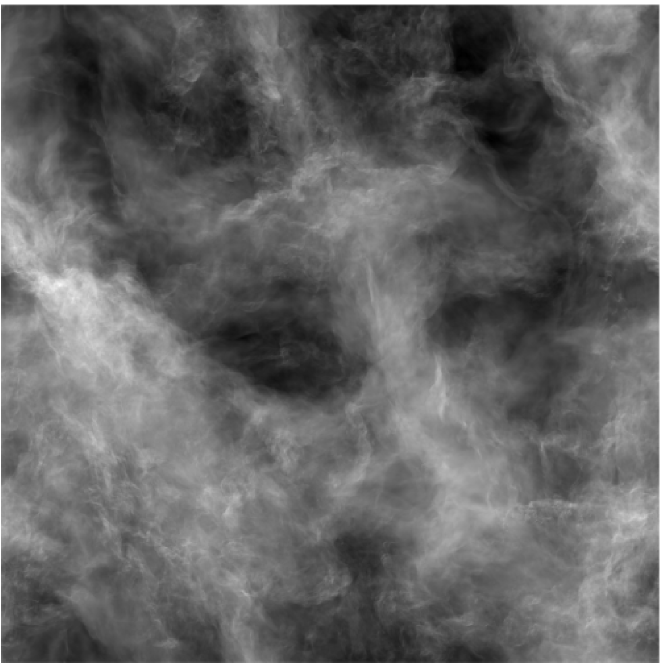
Figure 1: Projected mass density in an AMR simulation of supersonic turbulence with effective resolution $2048^{3}$ by Kritsuk et al.  2007, using Enzo [37]. Bright regions contain gas of high density, while under-dense gas appears dark.

In [37], the effective resolution (i. e. the resolution corresponding to the most refined grids) of an AMR simulation of supersonic turbulence was raised to the yet unprecedented value of $2048^{3}$. Nearly isothermal gas was maintained by setting the adiabatic exponent $\gamma$ to a value that differs only by a small fraction from unity. This means that the internal energy $E_{\mathrm{int}}=P/(\gamma-1)\rho$ is artificially increased by a huge factor such that $E_{\mathrm{int}}\gg\frac{1}{2}\rho v^{2}$ and, hence, it takes many dynamic time scales to heat the gas significantly by kinetic energy dissipation. In combination with a $1024^{3}$ static grid simulation, a great wealth of results was obtained from the analysis of the numerical data. Figure 1 shows the projected mass density in logarithmic scaling for one snapshot of the AMR simulation. One can see voids in between high-density regions which display intricate turbulent structure. This is a tell-tale sign of the pronounced intermittency of supersonic turbulence.

Further indications of intermittent properties come from the probability density function of the time-averaged mass density, which follows very closely a log-normal distribution [45], and the scaling exponents of the velocity structure functions. The definition of structure functions is based on spatial correlations of the velocity field:

$$S_{p}(\ell)=\langle|\boldsymbol{v}(\boldsymbol{x}+\boldsymbol{\ell})-\boldsymbol{v}(\boldsymbol{x})|\rangle^{p}.$$ (16)

The square brackets denote the average over the whole domain of the flow. Structure functions probe the correlations of the velocity field at different spatial positions depending on the separation $\ell$. It is both a theoretical prediction and an experimentally well established fact that the structure functions of isotropic turbulence obey power laws

$$S_{p}(\ell)\propto\ell^{\zeta_{p}}.$$ (17)

The exponents $\zeta_{p}$ are called the scaling exponents. For incompressible turbulence, Kolmogorov found $\zeta_{p}=p/3$. In the case of the second-order structure functions ($p$=2) this result corresponds to the $2/3$-law for the velocity fluctuations mentioned in Section 1. Calculating the scaling exponents form their numerical data, Kritsuk et al. were able to demonstrate significant deviations form the Kolmogorov relation in accordance with predictions of the intermittency model proposed by Boldyrev et al. [11, 37], which is a generalisation of the She-Lévêque model for incompressible turbulence [48]. In particular, it was found that $\zeta_{2}\approx 1.0$, whereas $\zeta_{2}=2/3$ in the Kolmogorov theory. Intriguingly, the analysis also revealed that the scaling exponents applicable to incompressible turbulence are obtained, if the statistics is computed for the density-weighted variable $\rho^{1/3}\boldsymbol{v}$ in place of $\boldsymbol{v}$, a result that is not fully understood yet but might bear important implications on the nature of supersonic turbulence.

3 Self-gravitating turbulence

According to the linear stability analysis of the Euler equations by Jeans [28], a perturbation in isothermal gas of temperature $T$ and uniform density $\rho_{0}$ becomes unstable against gravitational collapse, if its size exceeds the Jeans length

$$\lambda_{\mathrm{J}}=c_{\mathrm{s}}\sqrt{\frac{\pi}{G\rho_{0}}},$$ (18)

where $c_{\mathrm{s}}\propto T^{1/2}$ is the isothermal speed of sound. Beginning with Chandrasekhar’s proposition to substitute $c_{\mathrm{s}}^{2}$ by

$$c_{\mathrm{eff}}^{2}=c_{\mathrm{s}}^{2}+\frac{1}{3}\langle v^{2}\rangle$$ (19)

in the above expression for the Jeans length, several attempts have been made to extend the Jeans stability analysis to turbulent gas of RMS velocity $\langle v^{2}\rangle^{1/2}$ [16, 12, 13]. Equation (19) implies that the effective gas pressure is given by the sum of the thermal pressure $P$ and the turbulence pressure $P_{\mathrm{turb}}=\frac{2}{3}E_{\mathrm{kin}}$, where $E_{\mathrm{kin}}$ is the mean kinetic energy density.

However, even the most advanced analysis put forward so far [13], suffers from severe constraints. A perturbation analysis can be carried out for a statistically stationary equilibrium state only. Thus, it has to be assumed that the free fall time scale $T_{\mathrm{ff}}\sim(G\rho_{0})^{-1/2}$ is much greater than dynamical time scale of turbulent flow. From the divergence equation (10), one can see that this assumption implies that the self-gravity term remains small compared the other terms at all times. Allowing for gravitational collapse, however, self-gravity eventually dominates and

$$\frac{\mathrm{D}}{\mathrm{D}t}d\sim-G\rho.$$ (20)

A non-perturbative theory of the regime in which the free-fall time scale and the dynamical time scale of turbulence are comparable was suggested by Biglari and Diamond [8]. Combining scaling relations from the $\beta$-model of turbulence [22] with the assumption of energy equipartition between gravity and turbulence at all scales, they derived an intermittent hierarchical cloud model of self-gravitating turbulence.

At present, however, there is no general theory that would fully encompass the highly non-linear and non-stationary interplay between gravity and turbulence in the interstellar medium. Numerical simulations, on the other hand, can aid to the understanding self-gravitating turbulence, although one has to resort to artificial mechanisms of producing turbulence or imposing more or less arbitrary initial conditions. One technique is to apply a driving force as mentioned in the previous Section. Alternatively, some random initial velocity field might be assumed as initial condition. This results in decaying turbulence. Yet another option is to consider gas in an unstable state and apply small perturbations. The most prominent example is the thermal instability [35, 19].

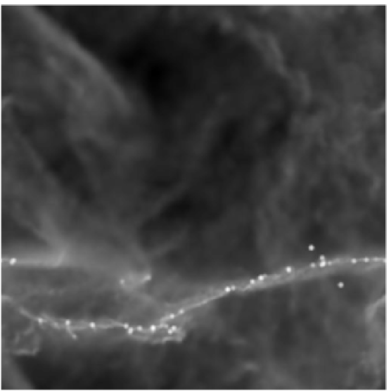
Figure 2: Filamentary structure with sink particles in an SPH simulation of self-gravitating turbulence (courtesy of R. Klessen). In this plot, over-dense regions appear bright.

Numerical simulations of self-gravitating driven or decaying supersonic turbulence were initially performed with smoothed particle hydrodynamics (SPH) because of its ability of tackle variations of the mass density over many orders of magnitude [41]. SPH makes use of the Lagrangian framework of fluid mechanics and represents fluid parcels by particles. Examples for the application of SPH to self-gravitating turbulence are the simulations by Klessen et al. [29, 30, 31]. In these simulations, the influence of self-gravity on probability density functions [29] and the fragmentation properties of the gas was investigated both for driven and for decaying supersonic turbulence [30, 31]. Sink particles were introduced to capture collapsing regions beyond a certain density threshold in order to prevent the mass density from growing indefinitely. Figure 2 illustrates that sink particles are mostly formed within filamentary structures (which are also seen in cosmological simulations). Varying the Mach number, it was found that higher turbulence intensity slows down the rate at which sink particles are produced considerably (Figure 3). The major conclusion drawn by Klessen et al. was that supersonic turbulence inhibits gravitational collapse globally, as one would suspect from equation (19). The strong gas compression caused by shocks, on the other hand, can trigger gravitational collapse locally and initiate the formation of stars.

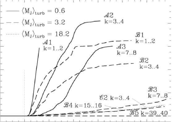
Figure 3: Total mass fraction captured by sink particles as a function of time in SPH simulations with different Mach numbers and varying driving scale of turbulence (Klessen et al., 2000 [30]).

Jappsen et al. [27] studied the mass spectrum produced by turbulent fragmentation in non-isothermal gas. They defined the state variables by piecewise polytropic relations, i. e. $P\propto\rho^{\gamma_{\mathrm{eff}}}$ for a certain range of densities. If $\gamma_{\mathrm{eff}}<1$, the gas cools with increasing density. This effect enhances the compressibility of the gas and therefore supports gravitational collapse (negative $\boldsymbol{\nabla}\rho\cdot\boldsymbol{\nabla}T$ contribution adds to the gravity term in the divergence equation 10) . At some threshold density, however, the cooling regime ceases and $\gamma_{\mathrm{eff}}$ becomes greater than unity. From various simulations, it was found that the transition from the cooling regime to isothermal or nearly isothermal gas sets a characteristic mass scale of turbulent fragmentation. This mass scale was interpreted to correspond to the peak of the observed initial mass function. Vàzquez-Semadeni et al. [55] included explicit heating and cooling in SPH simulations of colliding gas streams. They made use of a model for the cooling function $\Lambda$ in the energy equation (3) that was proposed by Koyama & Inutsuka [34]. Due to the thermal instability (compression causes the gas to cool), the gas at the collision interface undergoes gravitational collapse and becomes increasingly turbulent. This is interpreted as possible mechanism of molecular cloud formation. Remarkably, approximate equipartition of gravitational and kinetic energy was found, although clearly no state of virial equilibrium was approached by the collapsing gas. Further applications of SPH addressing problems such as the formation of brown dwarfs, binary star systems and stellar clusters via turbulent fragmentation as well as the origin of the initial mass function were presented by Bate et al. [3, 4, 5] and Bonnel et al. [14].

Despite the numerous important contributions to the understanding of the role of turbulence to star formation, the adequacy of treating turbulence with SPH has been a matter of debate. On the one hand, numerical studies of self-gravitating systems indicate basic agreement between AMR and SPH [18]. However, comparisons with grid-base codes suggest that SPH dissipates small-scale velocity fluctuations significantly stronger [46, 32]. In particular, it was demonstrated that the steeper power spectra obtained from SPH simulations are accompanied by mass distributions which are not consistent with observations. Apart from that, it appears to be rather difficult to accommodate magnetohydrodynamics in the SPH formalism. Although there are ongoing attempts to overcome this shortcoming [40], MHD has been treated with great success using finite-volume discretisation.

4 Magnetohydrodynamic turbulence

In purely hydrodynamical turbulence, there is no preferred spatial direction for small-scale velocity fluctuation. The randomisation of the flow due to non-linear turbulent interactions produces statistical isotropy towards small scales which can be interpreted as a symmetry of the ensemble average [22]. This symmetry is broken by a magnetic field $\boldsymbol{B}$ in turbulent conducting fluid, if the ratio of the thermal to the magnetic pressure,

$$\beta=\frac{P}{P_{\mathrm{M}}}=\frac{8\pi P}{B^{2}},$$ (21)

is comparable to unity or less. If the curl of the Lorentz force, $\boldsymbol{\nabla}\times(\boldsymbol{J}\times\boldsymbol{B})$, in the vorticity equation (9) is sufficiently strong, then the vorticity will mainly grow in the direction of $\boldsymbol{B}$. In developed magnetohydrodynamic (MHD) turbulence, this effect causes eddies to shrink perpendicular to the field lines. As a further implication, the anisotropy of MHD turbulence increases towards smaller length scales [9].

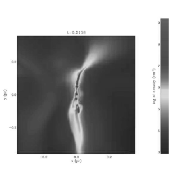
Figure 4: Simulation of a collapsing gas cloud of $1000$ solar masses with Ramses (courtesy of P. Hennebelle). The magnetic energy of the clouds is about the same as its kinetic energy.

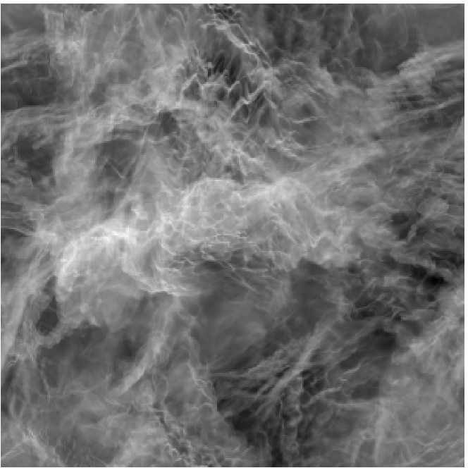
Figure 5: Projected mass density in a simulation of hydrodynamic turbulence with the Stagger code (Padoan et al., 2007 [46]). For comparison with MHD turbulence, see Figure 6

.

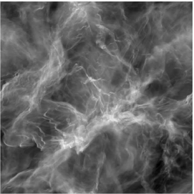
Figure 6: Projected mass density in a simulation of magnetohydrodynamic turbulence with the Stagger code (Padoan et al., 2007 [46]). For comparison with purely hydrodynamic turbulence, see Figure 5

.

The numerical simulation of MHD turbulence is rather challenging. Godunov-based schemes of higher order such as PPM become very complex upon including MHD. For this reason, simpler schemes have been adopted for MHD. Examples are the Zeus code [52], the Stagger code [43], and the Ramses code which also features AMR [54, 23]. As an illustration, Figure 4 shows a simulation of the gravitational collapse of a magnetised cloud with up to 6 levels of refinement. One of the major problems that needs to be addressed when solving the MHD equations numerically is to keep the magnetic field divergence-free, i. e. $\boldsymbol{\nabla}\cdot\boldsymbol{B}=0$. In Ramses and other codes, the constrained transport algorithm is employed to ensure this constraint [21].

A comparison of the properties of driven hydrodynamic (HD) and MHD turbulence in high-resolution simulations was presented by Padoan et al. [46]. Whereas the energy spectrum functions, irrespective of magnetic fields, were found to follow closely the power law $k^{-2}$ in the inertial subrange, the fragmentation properties of the gas appear to be markedly different for HD and MHD turbulence, respectively. In plots of the projected density fields for both cases (Figures 5 and 6), one can see that the gas is more concentrated in pronounced filaments under the action of magnetic fields. Utilising a clump-find algorithm, it was demonstrated that a significantly steeper mass spectrum of dense cores (defined by a density threshold based on the Bonnor-Ebert mass) resulted from purely hydrodynamical turbulence. Furthermore, they were able to reproduce the Chabrier initial mass function [15] in the MHD case, although this result must be considered with care given the ambiguity of calculating mass spectra.

Glover and Mac Low [24] performed simulations of self-gravitating MHD turbulence including various thermal and chemical processes. They were able to show that the fast formation of molecular hydrogen within a few Myrs, which is typically observed in molecular clouds, can be explained as an effect of turbulence. Hennebelle & Audit [26] investigated thermally bistable MHD turbulence and found mass spectra similar to those inferred from CO observations of molecular clouds. Although first computed in only 2 dimensions, the setup was generalised to include self-gravity and computed in 3 dimensions as well. The ansatz by Hennebelle et al. is different from simulations of isothermal MHD turbulence as it does not rely on a driving force or an initial turbulent velocity field.

 

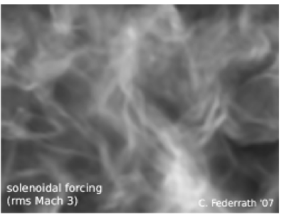
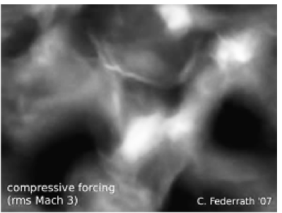
Figure 7: Projected mass density in $128^{3}$ simulations of turbulence driven by a solenoidal and a compressive force field, respectively (courtesy of C. Federrath).

5 Perspectives

Up to now, most approaches to the numerical simulation of astrophysical turbulence have focused on particular aspects, be it a thorough understanding of supersonic turbulence, the study of the dynamics of self-gravitating turbulent gas or an emphasis on the effects of magnetic fields. While impressive progress has been made in the area of isotropic turbulence, both in the HD and the MHD case, more complex scenarios remain elusive. The treatment of thermal and chemical processes is still fairly approximate. Our understanding of self-gravitating turbulence remains poor, despite many ongoing efforts. Radiation HD and MHD in combination with adaptive methods, are just beginning.

There is one aspect that should be highlighted whenever we are talking about the simulation of turbulence in the interstellar medium. The huge range of length scales from the galactic disk down to proto-stellar cores does not allow for coverage by a single numerical simulation. In general, there are two numerical cutoffs, one toward larger scales, the other toward smaller scales. The former poses the question of initial as well as boundary conditions and whether simple models such as periodic boxes and random forcing can account for those in a self-consistent fashion. The small-scale cutoff would, in general, necessitate closures. These are considered as essential in atmospheric sciences but have met very little attention in astrophysics.

As regards the large scales, it certainly will not be feasible in the near future to run a simulation of a disk galaxy or even a piece of a galactic disks including all processes of turbulence production, the different phases of the interstellar medium, the formation of molecular clouds and the collapse of gas giving rise to the birth of stars. If energy is injected via radom forcing in a simulation of turbulence over some subrange of scales in the ISM, one faces the question of what the influence of the forcing might be. That the outcome can vary depending on the applied forcing is illustrated by a simple numerical experiment. Figure 7 shows projected mass densities obtained from $128^{3}$ simulations, in which purely solenoidal (left) and compressive (right) forcing was applied. Although there is no fully developed turbulence at such low resolution, the plots suggest that the flow morphology is genuinely different, with markedly higher density contrasts and more pronounced intermittency in the case of compressive forcing. Indeed, this conclusion is confirmed by high-resolution simulations [51].

For the high-fidelity treatment of small scale effects, AMR emerges as the most promising tool, simply following the maxim to go to very high levels of refinement wherever the critical events take place. This was most impressively executed by Abel et al. [1] in AMR simulations of the formation of the first stars in the Universe. However, circumstances are not that favourable when it comes to galactic star formation and it remains to be seen whether AMR by itself will hold its promises. An alternative approach was suggested by Niemeyer et al. [42]. The basic idea is to combine the techniques of AMR, which have been brought to great success in astrophysics, and subgrid scale modelling, which is commonly used in engineering. Furthermore, the incorporation of additional physics such as thermal processes, complex chemistry as well as radiation transport in AMR simulations are essential for realistic models of turbulence in the ISM.

References

- [1] Abel, T., Bryan, G.L. and Norman, M.L. (2002). The Formation of the First Star in the Universe, Science 295, 93–98.
- [2] Ballesteros-Paredes, J., Gazol, A., Kim, J., Klessen, R.S., Jappsen, A.-K. and Tejero, E. (2006). The Mass Spectra of Cores in Turbulent Molecular Clouds and Implications for the Initial Mass Function, The Astrophysical Journal 637(1), 384–391.
- [3] Bate, M. R., I. A. Bonnell, and V. Bromm (2002a). The formation mechanism of brown dwarfs, Mon. Not. R. Astron. Soc. 332, L65-L68.
- [4] Bate, M. R., I. A. Bonnell, and V. Bromm, (2002b), The formation of close binary systems by dynamical interactions and orbital decay, Mon. Not. R. Astron. Soc. 336, 705–713.
- [5] Bate, M. R. and I. A. Bonnell (2005). The origin of the initial mass function and its dependence on the mean Jeans mass in molecular clouds, Mon. Not. R. Astron. Soc. 356(4), 1201–1221.
- [6] Berger, M. J. and Oliger, J. (1984). Adaptive Mesh Refinement for Hyperbolic Partial Differential Equations, J. Comp. Physics 53, 484–512.
- [7] Berger, M. J. and Colella, P. (1989). Local Adaptive Mesh Refinement for Shock Hydrodynamics. J. Comp. Physics 82, 64–84.
- [8] Biglari, H. and Diamond, P.H. (1989). Clouds and holes: Self-organization in compressible fluid and collisionless plasma turbulence, Physica D 37, 206–214.
- [9] Biskamp, D. (2003). Magnetohydrodynamic Turbulence, Cambridge University Press.
- [10] Boldyrev, S. (2002). Kolmogorov-Burgers Model for Star-forming Turbulence. Astrophys. J. 569, 841–845.
- [11] Boldyrev, S., Nordlund, A. and Padoan P. (2002). Scaling Relations of Supersonic Turbulence in Star-forming Molecular Clouds. Astrophys. J. 573, 678–684.
- [12] Bonazzola, S., Falgarone, E., Heyvaerts, J., Perault, M. and Puget, J. L. (1987). Jeans collapse in a turbulent medium, Astron. Astrophys. 172, 293–+.
- [13] Bonazzola, S., Perault, M., Puget, J. L., Heyvaerts, J., Falgarone, E. and Panis, J. F. (1992). Jeans collapse of turbulent gas clouds - Tentative theory, J. Fluid Mech. 245, 1–+.
- [14] Bonnell, I.A., Bate, M.R. and Vine, S.G. (2003). The hierarchical formation of a stellar cluster, Mon. Not. R. Astron. Soc. 343(2), 413–418.
- [15] Chabrier, G. (2003). Galactic Stellar and Substellar Initial Mass Function, PASP 115, 763–+.
- [16] Chandrasekhar, S. (1951). The gravitational instability of an infinite homogeneous turbulent medium, Proc. R. Soc. London A 210, 26–+.
- [17] Colella, P. and Woodward, P.R. (1984). The piecewise parabolic method (PPM) for gas-dynamical simulations, J. Comp. Physics 54, 174–201.
- [18] Commercon, B., Hennebelle, P., Audit, E., Chabrier, G. and Teyssier, R. (2007). Numerical methods comparison for protostellar collapse calculations, to appear in proceedings of SF2A-2007: Semaine de l’Astrophysique Francaise (J. Bouvier, A. Chalabaev, and C. Charbonnel eds.), eprint arXiv:0709.2450
- [19] Elmegreen, B.G. and Scalo, J. (2004). Interstellar Turbulence I: Observations and Processes, Ann. Rev. Astron. Astrophys. 42(1), 211–273.
- [20] Euler, L. (1757). Principes généraux du mouvement des fluides, Königliche Akademie der Wissenschaften, Berlin.
- [21] Evans, C. and Hawley, J. (1988). Simulation of magnetohydrodynamic flows - A constrained transport method, Astrophys. J. 332, 659–677.
- [22] Frisch, U. (1995). Turbulence, Cambridge University Press.
- [23] Fromang, S., Hennebelle, P. and Teyssier, R. (2006). A high order Godunov scheme with constrained transport and adaptive mesh refinement for astrophysical magnetohydrodynamics, Astron. Astrophys. 457, 371–+.
- [24] Glover, S.C.O. and Mac Low, M.-M. (2007). Simulating the Formation of Molecular Clouds. II. Rapid Formation from Turbulent Initial Conditions, Astrophys. J. 659,1317–1337.
- [25] Heisenberg, W. (1923). Über Stabilität und Turbulenz von Flüssigkeitsströmen, Doctoral Dissertation, Ludwigs-Maximillian-Universität München.
- [26] Hennebelle, P. and Audit, E. (2007) On the structure of the turbulent interstellar atomic hydrogen. I. Physical characteristics. Influence and nature of turbulence in a thermally bistable flow, Astron. Astrophys. 65(2), 431–443.
- [27] Jappsen, A.K., Klessen, R.S., Larson, R.B., Li, Y. and Mac Low, M.-M. (2005). The stellar mass spectrum from non-isothermal gravoturbulent fragmentation, Astron. Astrophys. 435(2) 611–623.
- [28] Jeans, J. H. (1902). The stability of a spherical nebula, Philos. Trans. R. Soc. London A 199, 1.
- [29] Klessen, R.S. (2000a). One-Point Probability Distribution Functions of Supersonic Turbulent Flows in Self-gravitating Media, Astrophys. J. 535(2), 869–886.
- [30] Klessen, R.S., Heitsch, F. and Mac Low, M.-M. (2000) Gravitational Collapse in Turbulent Molecular Clouds. I. Gasdynamical Turbulence strophys. J. 535(2), 887–906.
- [31] Klessen, R.S. (2001). The Formation of Stellar Clusters: Mass Spectra from Turbulent Molecular Cloud Fragmentation Astrophys. J. 556(2), 837–846.
- [32] Kitsionas et al. in prep.
- [33] Kolmogorov, A. (1941). The Local Structure of Turbulence in Incompressible Viscous Fluid for Very Large Reynolds Numbers, Dokl. Akad. Nauk SSSR 30, 301–305
- [34] Koyama, H., Inutsuka, S.-I. (2002). An Origin of Supersonic Motions in Interstellar Clouds, Astrophys. J. 564(2), L97–L100.
- [35] Kritsuk, A.G. and Norman, M.L. (2002) Thermal Instability-induced Interstellar Turbulence, Astrophys. J. Lett. 569, L127–L131.
- [36] Kritsuk, A.G., Norman, M.L. and P. Padoan (2006). Adaptive Mesh Refinement for Supersonic Molecular Cloud Turbulence, Astrophys. J. Lett. 638, L25–L28.
- [37] Kritsuk, A.G., Norman, M.L., Padoan, P. and Wagner, R. (2007). The Statistics of Supersonic Isothermal Turbulence, Astrophys. J. 665, 416–431.
- [38] Landau L.D. and Lifshitz, E.M. (1987). Fluid Mechanics, Course of Theoretical Physics Vol. 6, 2nd edition, Pergamon Press.
- [39] Mac Low, M.-M. and Klessen, R.S. (2004). Control of star formation by supersonic turbulence, Rev. Modern Phys. 76(1), 125–194.
- [40] Maron, J.L. and Howes, G.G. (2003). Gradient Particle Magnetohydrodynamics: A Lagrangian Particle Code for Astrophysical Magnetohydrodynamics, Astrophys. J. 595(1), 564–572
- [41] Monaghan, J.J. (1992). Smoothed particle hydrodynamics, in Ann. Rev. Astron. Astrophys. 30, 543–574.
- [42] Niemeyer, J., Schmidt, W. and Klingenberg, C. (2005) The FEARLESS Cosmic Turbulence Projects, in Ringberg Proceedings on Interdisciplinary Aspects of Turbulence, MPA/P15, 175–181
- [43] Nordlund, Åand Galsgaard, K. (1995). A 3D MHD Code for Parallel Computers. Technical report, Astronomical Observatory, Copenhagen University.
- [44] O’Shea, B. W., Bryan, G., Bordner, J., Norman, M.L., Abel, T., Harkness, R. and Kritsuk, A. (2004). Introducing Enzo, an AMR Cosmology Application, in Adaptive Mesh Refinement - Theory and Applications, edited by T. Plewa, T. Linde & V. G. Weirs, Springer Lecture Notes in Computational Science and Engineering.
- [45] Padoan, P. and Nordlund, Å. (2007). The Stellar Initial Mass Function from Turbulent Fragmentation, Astrophys. J. 576, 870–879.
- [46] Padoan, P., Nordlund, Å., Kritsuk, A.G., Norman, M. L., and Li, P.S. (2007). The mass distribution of unstable cores in turbulent magnetized clouds, in Triggered Star Formation in a Turbulent ISM, edited by B. G. Elmegreen and J. Palous. Proceedings of the International Astronomical Union 2, IAU Symposium #237, held 14-18 August, 2006 in Prague, Czech Republic. Cambridge: Cambridge University Press, 283–291.
- [47] D. Porter, A. Pouquet, and P. Woodward (2002). Measures of intermittency in driven supersonic flows, Phys. Rev. E 66, 026301.
- [48] She, Z.-S. and Lévêque, E. (1994). Universal scaling laws in fully developed turbulence, Phys. Rev. E. 72, 336–339.
- [49] Schmidt, W., Hillebrandt, W. and Niemeyer, J. C. (2006). Numerical dissipation and the bottleneck effect in simulations of compressible isotropic turbulence, Comp. Fluids 35, 353–371.
- [50] Schmidt, W. and Federrath, C. (2007). A Parameter Study of Forced Supersonic Turbulence in Large Eddy Simulations, submitted to Phys. Rev. E.
- [51] Schmidt, W., Federrath, C., Hupp, M., Maier, A. and Niemeyer, J. (2007). Isothermal turbulence driven by compressive forcing, submitted to Astron. Astrophys.
- [52] Stone, J.M. and Norman, M.L. (1992). ZEUS-2D: A Radiation Magnetohydrodynamics Code for Astrophysical Flows in Two Space Dimensions. II. The Magnetohydrodynamic Algorithms and Tests, Astrophys. J. Suppl. 80, 791–+.
- [53] Sytine, I.V., Porter, D.H., Woodward, P.R., Hodson, S.W. and Winkler, K. (2000). Convergence Tests for the Piecewise Parabolic Method and Navier-Stokes Solutions for Homogeneous Compressible Turbulence, J. Comp. Physics 158, 225–+.
- [54] Teyssier, R. (2002). Cosmological hydrodynamics with adaptive mesh refinement. A new high resolution code called RAMSES, Astron. Astrophys. 385, 337–364.
- [55] Vàzquez-Semadeni, E., Gómez, G.C.; Jappsen, A.K., Ballesteros- Paredes, J., González, R.F. and Klessen, R.S. (2007). Molecular Cloud Evolution. II. From Cloud Formation to the Early Stages of Star Formation in Decaying Conditions, Astrophys. J. 657(2), 870–883.