Tunneling of interacting fermions in 1D systems

Using the self-consistent Hartree-Fock approximation for spinless electrons at zero temperature, we study tunneling of the interacting electron gas through a single $\delta$ barrier in a finite one-dimensional (1D) wire connected to contacts. Our results exhibit features known from correlated many-body models. In particular, the conductance decays with the wire length as $\propto L^{-2\alpha}$, where the power $\alpha$ is universal. We also show that a similar result for a wire conductance can be extracted from the persistent current ($I$) through the $\delta$ barrier in a 1D ring, where it is known that $I\propto L^{-1-\alpha}$.

PACS numbers: 73.23.-b, 73.61.Ey

Electron gas in a quantum wire is a realistic one-dimensional (1D) system. If a clean wire is biased by two macroscopic contacts with negligible electron back-scattering, the wire conductance is quantized as an integer multiple of $e^{2}/h$. This effect can be explained in the model of noninteracting electrons [1].

If a localized scatterer is introduced into the wire, quantization of conductance breaks down due to the electron backscattering from the scatterer. For non-interacting electrons, the conductance is given by Landauer formula as the electron transmission probability at the Fermi level [1]. However, the electron-electron (e-e) interaction alters the properties of the system qualitatively. In the Luttinger liquid model [2], the conductance of an infinite wire containing a single scatterer varies with temperature as $\propto T^{-2\alpha}$ for $T\rightarrow 0$, where the power $\alpha$ depends only on the e-e interaction. For repulsive interaction $\alpha$ is positive and reflection at zero temperature is perfect, no matter how strong or weak the scatterer is.

Matveev et al. [3] studied the Landauer conductance of the interacting 1D electron gas through a $\delta$ barrier in a wire with contacts. They replaced the many-body wave function by the Slater determinant of single-electron wave functions and analyzed the effect of the Hartree-Fock potential on the tunneling transmission. Assuming a weak e-e interaction of finite range, they derived the transmission using the renormalization group (RG). They confirmed the universal power law $T^{-2\alpha}$, this approach is believed to go beyond the Hartree-Fock approximation.

Here we consider the non-Luttinger liquid model of Matveev et al. [3], but instead of the RG approach we apply the self-consistent Hartree-Fock solution. We evaluate the Landauer conductance. We find a good agreement with the theory of Matveev et al. In particular, we simulate asymptotic dependence of the conductance on the wire length ($L$) for strong $\delta$ barriers and we reproduce the universal power law $\propto L^{-2\alpha}$. We also show that essentially the same wire conductance can be extracted from the persistent current ($I$) in a 1D ring, where $I\propto L^{-\alpha-1}$.

We consider a 1D gas of interacting spinless electrons in a wire of length $L$. The wire is positioned along the $x$ axis between $x=-L/2$ and $x=L/2$, both wire ends are connected to contacts. The single-electron wave functions $\psi_{k}(x)$, where $k$ is the electron wave vector, are described by the Hartree-Fock equation

$$\left[-\frac{\hbar^{2}}{2m}\ \frac{d^{2}}{dx^{2}}+\gamma\delta(x)+U_{H}(x)+U_{F}(k,x)\right]\psi_{k}(x)\\ =\varepsilon_{k}\,\psi_{k}(x),$$ (1)

where $\gamma\delta(x)$ mimics the localized scatterer positioned in the center of the wire,

$$U_{H}(x)=\\ \int\limits_{-L/2}^{L/2}dx^{\prime}\ V(x-x^{\prime})\int\limits_{-k_{F}}^{k_{F}}\frac{dk^{\prime}}{2\pi}\left[\left|\psi_{k^{\prime}}(x^{\prime})\right|^{2}-\left|\psi^{0}_{k^{\prime}}(x^{\prime})\right|^{2}\right]$$ (2)

is the Hartree potential induced by the $\delta$ barrier,

$$U_{F}(k,x)=-\frac{1}{\psi_{k}(x)}\int\limits_{-L/2}^{L/2}\!\!dx^{\prime}\ V(x-x^{\prime})\,\\ \int\limits_{-k_{F}}^{k_{F}}\!\!\frac{dk^{\prime}}{2\pi}\,\,\psi_{k}(x^{\prime})\psi^{*}_{k^{\prime}}(x^{\prime})\,\psi_{k^{\prime}}(x)$$ (3)

is the Fock nonlocal exchange term, and $V(x-x^{\prime})$ is the e-e interaction.

The Landauer conductance is defined for the wire connected to large contacts via adiabatically tapered non-reflecting connectors [1]. First assume a clean non-interacting wire, i.e., $\gamma=0$ and $V(x-x^{\prime})=0$. As there is no backscattering at the wire ends, the solution of the equation (1) is the free wave $e^{ikx}$ with eigenenergy $\hbar^{2}k^{2}/2m$. The states $e^{ikx}$ and $e^{-ikx}$ with $k>0$ describe the ballistic electrons originating from the contact at $x=-L/2$ and $x=L/2$, respectively. As they are mutually incoherent, $e^{ikx}$ and $e^{-ikx}$ are the only independent solutions.

Second, let us keep $\gamma=0$ but let us turn on the e-e interaction $V(x-x^{\prime})$. Assuming that there is no backscattering at the wire ends, the solution of equation (1) is still the free wave, $\psi^{0}_{k}(x)=e^{ikx}$, but with the eigenenergy

$$\varepsilon_{k}=\hbar^{2}k^{2}/2m+U_{F}^{0}(k),$$ (4)

where $U_{F}^{0}(k)\equiv U_{F}[\psi_{k}(x)=\psi^{0}_{k}(x)]$ is the Fock shift. Note that this solution is valid if we implicitly assume that the Fock interaction is present also in the contacts. Indeed, if the energy (4) holds inside the wire and we turn off the Fock shift to zero outside the wire, we obtain at each wire end the potential drop $U_{F}^{0}(k)$. This would cause backscattering at both wire ends and the solutions $e^{ikx}$ and $e^{-ikx}$ would be no longer valid, in contrast with the ballistic conductance of clean wires [1].

Finally, consider the barrier $\gamma\delta(x)$ and interaction $V(x-x^{\prime})$. The $\delta$ barrier induces Friedel oscillations of the Hartree-Fock potential. The electrons are thus scattered by the $\delta$ barrier and by the oscillating potential relief. Since the scattering is elastic, the eigenenergy (4) remains unchanged and the wave function $\psi_{k}(x)$ can be found by solving equation (1) as a tunneling problem with boundary conditions

$$\psi_{k}(x=-L/2)=e^{ikx}+r_{k}e^{-ikx},\ \quad\quad\quad\psi_{k}(x=L/2)=t_{k}e^{ikx},$$ (5)

$$\psi_{-k}(x=-L/2)=t^{\prime}_{k}e^{-ikx},\ \quad\psi_{-k}(x=L/2)=e^{-ikx}+r^{\prime}_{k}e^{ikx},$$ (6)

where $k>0$, $r_{k}$ is the reflection amplitude, and $t_{k}$ is the transmission amplitude. Once we know the transmission, we know the Landauer conductance $(e^{2}/h)\left|t_{k_{F}}\right|^{2}$.

In reality the Friedel oscillations penetrate through the wire ends into the contacts, where they decay fast due to the enhanced dimensionality and decoherence. To mimic this decay within our 1D model, we sharply turn off the oscillations to zero at both wire ends and keep $U_{H}=0$ and $U_{F}=U_{F}^{0}(k)$ outside the wire. This constant 1D potential emulates the non-reflecting connectors and justifies the above boundary conditions. Essentially the same 1D model was a starting point of the RG study by Matveev et al. [3].

Unlike to Matveev et al., we solve the equation (1) by means of the self-consistent iterative procedure. To save the computational time and memory, we follow Ref. [4] and simplify the equation (3) as

$$U_{F}(x)\simeq-\int\limits_{-L/2}^{L/2}dx^{\prime}\ V(x-x^{\prime})\,\int\limits_{-k_{F}}^{k_{F}}\frac{dk^{\prime}}{2\pi}\,\text{Re}[\psi^{*}_{k^{\prime}}(x^{\prime})\,\psi_{k^{\prime}}(x)]$$ (7)

by noticing that $\int_{-k_{F}}^{k_{F}}dk^{\prime}\psi^{*}_{k^{\prime}}(x^{\prime})\,\psi_{k^{\prime}}(x)\simeq 2\pi\delta(x-x^{\prime})$. Unlike the exact form (3), the Fock potential (7) is local and independent on $k$. This saves time and allows us to simulate long wires. We present numerical results for the GaAs wire with electron density $n=5\times 10^{7}$ m^-1, effective mass $m=0.067$ $m_{0}$, and e-e interaction

$$V(x-x^{\prime})=V_{0}\,e^{-\left|x-x^{\prime}\right|/d}.$$ (8)

We adopt the finite-ranged interaction (8) because of comparison with the RG theory of Ref. [3] which also assumes the e-e interaction of finite range. Physical meaning of the finite range is screening.

According to Ref. [3] the bare $\delta$ barrier, described by the transmission and reflection amplitudes $\tilde{t}_{k}$ and $\tilde{r}_{k}$, is renormalized by the Friedel oscillations. The renormalized transmission probability at the Fermi level reads

$$\left|{t}_{k_{F}}\right|^{2}=\frac{\left|\tilde{t}_{k_{F}}\right|^{2}\,(d/L)^{2\alpha}}{{\left|\tilde{r}_{k_{F}}\right|^{2}+\left|\tilde{t}_{k_{F}}\right|^{2}\,(d/L)^{2\alpha}}}\simeq\frac{\left|\tilde{t}_{k_{F}}\right|^{2}}{|\tilde{r}_{k_{F}}|^{2}}\left(d/L\right)^{2\alpha},$$ (9)

where $d$ is the range of the e-e interaction $V(x-x^{\prime})$ and the right hand side of (9) holds for small $\tilde{t}_{k_{F}}$ and/or large $L$. For weak e-e interaction ($\alpha\ll 1$) $\alpha$ reads

$$\alpha=\frac{V(0)-V(2k_{F})}{2\pi\hbar v_{F}},$$ (10)

where $V(q)$ is the Fourier transform of the e-e interaction $V(x-x^{\prime})$. We evaluate $\alpha$ for our e-e interaction (8), for which $V(q)=2V_{0}d/(1+q^{2}d^{2})$.

The bare amplitudes are $\tilde{t}_{k}=k/(k+i\zeta)$ and $\tilde{r}_{k}=-i\zeta/(k+i\zeta)$, where $\zeta=\gamma m/\hbar^{2}$. Since $k_{F}$ and $m$ are fixed, in the following we parametrize the bare $\delta$ barrier by its transmission coefficient $\left|\tilde{t}_{k_{F}}\right|^{2}$.

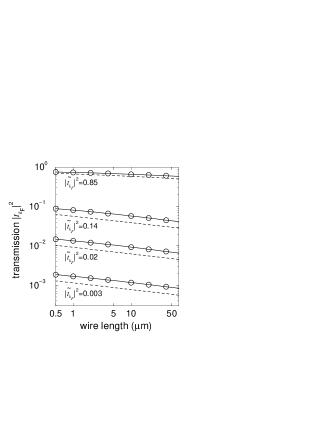
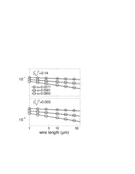
Figure 1: Transmission probability at the Fermi level versus wire length for various $\delta$ barriers $\left|\tilde{t}_{k_{F}}\right|^{2}$ and various e-e interaction strengths $\alpha$. The dashed curves show the data due to the RG formula (9); these data follow the asymptotic power law $\left|t_{k_{F}}\right|^{2}\propto L^{-2\alpha}$ as the $\delta$ barrier becomes strong. The circles connected by the full lines are our self-consistent Hartree-Fock data; they approach the same asymptotic power law. The powers $\alpha=0.0277$, $0.0561$, and $0.0855$ correspond to $V_{0}=11$ meV, $22.3$ meV, and $34$ meV, respectively, with $d$ fixed to $3$ nm. If we adjust the same $\alpha$ by another choice of $V_{0}$ and $d$, our results remain unchanged.

Figure 1 shows the transmission probability $\left|{t}_{k_{F}}\right|^{2}$ versus the wire length $L$ for various $\delta$ barriers and various e-e interaction strengths. The RG formula (9) is presented by the dashed lines. For strong $\delta$ barriers the dashed lines follow the asymptotic power law $\left|t_{k_{F}}\right|^{2}\propto L^{-2\alpha}$, in the log scale manifested by linear decay with slope $-2\alpha$. Our Hartree-Fock curves (open symbols connected by full lines) show slightly higher transmission but clearly follow the same trend. In particular, for small enough $\left|\tilde{t}_{k_{F}}\right|^{2}$ and for not too small $L$ all Hartree-Fock curves decay with the same slope as the RG curves, independently on the strength of the $\delta$ barrier.

It is instructive to show the Hartree-Fock potential $U_{H}(x)+U_{F}(x)$ in the form

$$U_{HF}(y)=(d/L)^{\alpha}[U_{H}(y)+U_{F}(y)-U_{F}^{0}]/\Delta_{L}\,,\quad y=x/L\,,\quad\Delta_{L}=\pi\hbar v_{F}/L,$$ (11)

where we subtract the constant Fock shift $U_{F}^{0}$ in order to show exclusively the Hartree-Fock potential induced by the $\delta$ barrier.

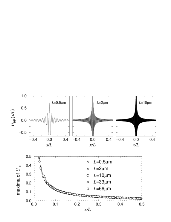
Figure 2: Self-consistent Hartree-Fock potential $U_{HF}(x/L)$ along a 1D wire, induced by the (not shown) $\delta$ barrier at $x=0$. The $\delta$ barrier is adjusted to have the transmission $\left|\tilde{t}_{k_{F}}\right|^{2}=0.003$ at the Fermi level ($14$ meV). The wire length, $L$, is varied as a parameter. The bottom panel shows just the positive maxima of the Friedel oscillations.

In Fig. 2 we show the typical self-consistent $U_{HF}(y)$ in the wire with a strong scatterer at $y=0$. The potential exhibits Friedel oscillations with period $\lambda_{F}/2L$. The bare scatterer is thus “dressed” by an extra scatterer due to the Friedel oscillations. This is why we see the conductance to decay with $L$. It is more difficult to understand why we see just $\left|t_{k_{F}}\right|^{2}\propto(d/L)^{2\alpha}$. As $L$ increases, the Friedel oscillations in Fig. 2 are too dense to be distinguishable, but we can observe asymptotic decay of the oscillation amplitude. Notice that the “envelope” of the oscillation amplitude is the same for all $L$. Indeed, as shown in the bottom panel, the “envelope” scales for all $L$ to a single curve. Notice also (c.f. eq. (11)), that $U_{HF}(y)$ involves the scaling factor $(d/L)^{\alpha}$. This might be the reason why $\left|t_{k_{F}}\right|^{2}\propto(d/L)^{2\alpha}$, but we have so far not found a clear interpretation.

By tying the wire ends to each other one can create the 1D ring. Magnetic flux applied through the opening of the ring gives rise to the equilibrium persistent current. In our paper [5] we have calculated the persistent current in the 1D ring with a single $\delta$ barrier. We have applied the same Hartree-Fock model as in this work, except that the Hartree-Fock equation with cyclic boundary condition [5] is the eigenvalue problem rather than the tunneling problem.

Figure 3: (a) The $U_{HF}$ data from the Fig 2. (b) Analogous data for the 1D ring from our paper [5]. (c) Maxima of $U_{HF}$ for the wire (full line) and ring (dashed line). (d) The same as in the panel (c) but in log scale.

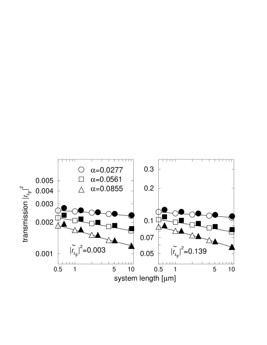
Figure 4: The transmission probability for the 1D wire (the open symbols represent the data from Fig. 1) compared with the transmission probability extracted from the persistent current of the 1D ring (full symbols). The left and right panels show the transmission probability for $\left|\tilde{t}_{k_{F}}\right|^{2}=0.003$ and $\left|\tilde{t}_{k_{F}}\right|^{2}=0.139$, respectively.

In Fig. 3 we compare the Hartree-Fock potentials in the wire and ring. Obviously, the amplitude of the Friedel oscillations in the ring saturates at the boundaries. However, the amplitude of the Friedel oscillations in the wire decays with distance from the scatterer without any tendency to saturate (note in panel (d), that the decay of the full line in log scale is linear or even slightly faster than linear). Nevertheless, in both cases $U_{HF}(y)$ involves the scaling factor $(d/L)^{\alpha}$ and the “envelope” scales to a single curve for all $L$. It is thus not surprising, that also the persistent current in the ring ($I$) comes out from the Hartree-Fock model [5] as a power law, namely $LI\propto(d/L)^{\alpha}$. This suggests that the conductance of the interacting wire might be obtainable from the persistent current in the interacting ring. In the non-interacting case $I=(ev_{F}/2L)|\tilde{t}_{k_{F}}|$ for magnetic flux $0.25h/e$. Applying this formula (intuitively) to the interacting electrons, we obtain the wire conductance from the formula $|{t}_{k_{F}}|^{2}=2LI/ev_{F}$, with $I$ taken from the persistent current simulation [5]. In Fig. 4 we show that the results (full symbols) reasonably agree with our direct calculation of the wire conductance.

In conclusion, using the self-consistent Hartree-Fock approximation at zero temperature, we have calculated the Landauer conductance of the weakly-interacting spinless electron gas in a 1D wire with a single $\delta$ barrier. We have found the universal power law $\left|t_{k_{F}}\right|^{2}\propto(d/L)^{2\alpha}$ known from the Luttinger-liquid model [2] and RG models [3, 6]. We have also found that essentially the same wire conductance can be extracted from the persistent current in a 1D ring.

We thank for the APVT grant APVT-51-021602 and VEGA grant 2/3118/23.

References

- [1] S. Datta, Electronic Transport in Mesoscopic Systems (Cambridge University Press, Cambridge, UK, 1995).
- [2] C. L. Kane and M. P. A. Fisher, Phys. Rev. Lett. 68, 1220 (1992).
- [3] K. A. Matveev, D. Yue, L. I. Glazman, Phys. Rev. Lett. 71, 3351 (1993).
- [4] A. Cohen, R. Berkovits, A. Heinrich, Int. J. Mod. Phys. B 11, 1845 (1997).
- [5] R. Németh and M. Moško, these proceedings.
- [6] V. Meden, W. Metzner, U. Schollwöck, and K. Schönhammer, Phys. Rev. B 65, 045318 (2002).