Finite de Finetti theorem for conditional probability distributions describing physical theories

Abstract

We work in a general framework where the state of a physical system is defined by its behaviour under measurement and the global state is constrained by no-signalling conditions. We show that the marginals of symmetric states in such theories can be approximated by convex combinations of independent and identical conditional probability distributions, generalizing the classical finite de Finetti theorem of Diaconis and Freedman. Our results apply to correlations obtained from quantum states even when there is no bound on the local dimension, so that known quantum de Finetti theorems cannot be used.

I Introduction

Given a bowl containing $n$ colored balls, we wish to compare two ways of obtaining a random sample of $k\leq n$ balls: (i) we randomly choose a ball, replace it with a ball of the same color, and repeat this step $k$ times; (ii) we do the same but don’t replace the balls. If $k\ll n$, then the probability of obtaining a particular set of $k$ balls will be almost the same in both cases Diaconis and Freedman (1980). This observation has profound consequences for Bayesian statistical inference, as we now describe.

Suppose we perform an experiment $k$ times in order to estimate some physical quantity, e.g., the probability $\lambda$ that a muon decays in a given time. Let $A_{i}=1$ if the $i$th muon decayed and $A_{i}=0$ if it did not. If we assume that the results of the experiments are independent, we can posit some prior probability distribution $m(\lambda)$ and analyze our data by updating this probability distribution as more data arrives. Statisticians of de Finetti’s subjective school Bernardo and Smith (1994) are not willing to accept this assumption, however, since for them all probability distributions should be subjective degrees of belief, which $m(\lambda)$ is not. Instead, they make the weaker assumptions that the experiment could have been performed $n\gg k$ times and that there was nothing special about the experiments actually performed. These assumptions, together with the observation about colored balls above, can be shown to imply that there exists a distribution $m(\lambda)$ such that

$$P[A_{1},\ldots,A_{k}]\approx\int dm(\lambda)P_{\lambda}[A_{1}]\cdots P_{\lambda}[A_{k}],$$ (1)

i.e., the probability distribution $P[A^{k}]$ behaves as if the experiments really were independent and there really were some objective prior $m(\lambda)$. This is a statement of the famous de Finetti representation theorem de Finetti (1937); Diaconis and Freedman (1980). Our results establish the same correspondence for measurement results in a more general, probabilistic, physical theory, where the state of a system is described by a conditional probability distribution.

We now give a brief description of the setting and our results; precise definitions are given later on. A physical system in a probabilistic physical theory is made up of a number of—in our case identical—subsystems, called particles. On each particle different measurements from a set $\mathcal{X}$ can be performed and outputs from a set $\mathcal{A}$ are obtained. The state of a particle is specified by a conditional probability distribution $P[A|X]$: the probability of obtaining result $a$ when performing measurement $x$ is given by $P[A=a|X=x]$. The possible states of $n$ particles are the conditional probability distributions $P[A^{n}|X^{n}]$ that obey a no-signalling property, which ensures that the reduced state on a subset of the particles is always well-defined.

Our main result is that the joint state $P[A^{k}|X^{k}]=P[A_{1}\cdots A_{k}|X_{1}\cdots X_{k}]$ of $k$ particles randomly chosen from $n$ particles—or equivalently, the state of the first $k$ particles of a permutation-invariant state of $n$ particles—can be approximated by a convex combination of identical and independent conditional probability distributions,

$$P[A^{k}|X^{k}]\approx\int dm(\lambda)P_{\lambda}[A|X]^{\times k}$$ (2)

and that the error in the approximation is bounded by $|\mathcal{X}|k(k-1)/n$ in the appropriate distance measure, where $|\mathcal{X}|$ is the number of different possible measurements. (We write $P_{\lambda}[A|X]^{\times k}$ for $P_{\lambda}[A_{1}|X_{1}]\cdots P_{\lambda}[A_{k}|X_{k}]$.) Our result generalizes the finite de Finetti theorem of Diaconis and Freedman, who proved for classical probability distributions ($|\mathcal{X}|=1$) that the error in the approximation is no more than $k(k-1)/n$ Diaconis and Freedman (1980) .

This paper is motivated by recent work on finite quantum de Finetti theorems, i.e., statements of the form

$$\rho^{k}\approx\int d\sigma\ \sigma^{\otimes k},$$ (3)

where $\rho^{k}$ is the $k$-particle reduced density matrix of a permutation-invariant density matrix of $n$ particles with state space of dimension $d$, where the error is at most $4d^{2}k/n$ in the trace distance König and Renner (2005); Christandl et al. (2007) . In fact, it is necessary that the error depends on $d$ Christandl et al. (2007), and so the quantum de Finetti is not useful in applications where $d$ cannot be bounded. Our results are designed to apply in this setting: provided we have a bound on the number of ways $|\mathcal{X}|$ that a system is measured, the approximation in Eq. (2) will be good, even if there is no bound on the local dimension $d$. In recent years, quantum de Finetti theorems, especially Renner’s so-called ‘exponential’ version Renner (2005), have been used to prove the security of quantum key distribution (QKD) schemes Bennett and Brassard (1984). At the same time, attempts have been made to lift the assumption of a fixed (finite) local dimension Acín et al. (2007). Since quantum de Finetti theorems are necessarily dimension-dependent, they cannot be used in this setting. Although our theorems do not directly lead to security proofs either, we regard them as a first step towards this goal.

We also prove a finite quantum de Finetti theorem for separable $\rho^{n}$: in this case there is an approximation of the form in Eq. (3) with error $k(k-1)/n$, independent of the dimension. We do not, however, know whether our techniques can be extended to prove the finite quantum de Finetti theorem in full generality. The issue is that our theorem concerns conditional probability distributions that arise from measuring quantum states and not the quantum states themselves. If we take, for example, a tomographically complete set of measurements, the representation described in Eq. (2) will in general contain distributions $P_{\lambda}[A|X]$ that cannot be obtained by performing the tomographic measurements on quantum states. One can, however, apply the argument of Caves et al. (2002) to obtain the infinite quantum de Finetti theorem and indeed an infinite de Finetti theorem for any physical theory in what is known as the convex sets framework Barnum et al. (2006, 2007) (see Barrett and Leifer (2007) for the details).

Another application of our work is to the study of classical channels. Fuchs, Schack and Scudo have used the Jamiolkowski isomorphism to transfer the infinite quantum de Finetti theorem ($n=\infty$, $k<\infty$) Størmer (1969); Caves et al. (2002) to quantum channels Fuchs et al. (2004). Since a conditional probability distribution can be viewed as a classical channel with probability distributions as input and output, our results also provide a de Finetti theorem for classical channels.

Outline.—Our first task is to define an appropriate distance measure on states of $k$ particles in probabilistic theories, in order to quantify the error in Eq. (2). The distance between states should bound the probability of distinguishing them by measurement, and so we need to be clear about what measurement strategies are allowed. One possibility, which we explore in Christandl and Toner (2009), is to restrict to strategies where each of the $k$ particles is measured individually. But when the conditional probability distributions arise from making informationally complete local measurements on entangled quantum states, the resulting distance measure fails to bound the trace distance between the quantum states. In the next section we show how to define a ‘good’ distance measure in which all noncontextual measurements are allowed, including all joint quantum-mechanical measurements. We then state and prove our results. In the last section, we explain the origin of the distance measure, the convex sets framework, which allows us to conclude with an open question on finite de Finetti theorems in this more general setting.

II A distance measure for conditional probability distributions

When we measure a quantum system, the probability of obtaining an outcome $a\in\mathcal{A}$ depends on which measurement $x\in\mathcal{X}$ we choose to perform on the system. It is usual to describe a quantum system using the formalism of density matrices, Hilbert spaces, and so on, but we can also describe the system by specifying a conditional probability distribution $P[A|X]$, where we write $P[A|X=x]$ for the distribution of measurement outcome $A$ given that measurement $x$ is performed . While a classical system can be described using an unconditional probability distribution, the same is not true for a quantum system, since measuring a quantum system disturbs it, eliminating our ability to make a second, incompatible, measurement on the same system.

We are therefore motivated to describe the state of an abstract system (not necessarily obeying quantum theory) using a conditional probability distribution $P[A|X]$. We view the conditional probability distribution $P[A|X]$ as the output distribution of a measurement that has been performed on system $A$. Alternatively, one can view $P[A|X]$ as a channel that produces an output distribution $P[A|X=x]$ on input $x$. For this reason we refer to the measurement setting $x$ as the input and the measurement result $a$ as the output. Generalizing from conditional probability distributions of one system, we shall consider a conditional probability distribution $P[A^{n}|X^{n}]=P[A_{1}\cdots A_{n}|X_{1}\cdots X_{n}]$, which describes an abstract system composed of $n$ subsystems, which we call particles.

We need to be able to describe the state of a subset $\mathcal{I}\subset\{1,\ldots,n\}$ of the particles. Taking the marginal of a conditional probability distribution $P[A^{n}|X^{n}]$ yields a conditional distribution $P[A_{\mathcal{I}}|X^{n}]$, where the outputs at the particles in $\mathcal{I}$ depends on the inputs at all $n$ sites. In order to trace out the particles that are not in $\mathcal{I}$ entirely, rather than just the outputs obtained from measuring them, we need another notion, that of a conditional probability distribution being no-signalling.

Definition 1.

A conditional distribution $P[A^{n}|X^{n}]$ is no-signalling if for all subsets $\mathcal{I}\subset\{1,\ldots,n\}$ with complements $\bar{\mathcal{I}}:=\{1,\ldots,n\}\backslash\mathcal{I}$

$$P[A_{\mathcal{I}}=a_{\mathcal{I}}|X_{\mathcal{I}}=x_{\mathcal{I}}]\mathrel{\mathop{:}}=\sum_{a_{\bar{\mathcal{I}}}}P[A^{n}=a^{n}|X^{n}=x^{n}]$$ (4)

is independent of $x_{\bar{\mathcal{I}}}$ for all $a_{\mathcal{I}}$ and all $x_{\mathcal{I}}$.

The terminology derives from the following fact: if we divide the $n$ parties into two groups, $\mathcal{I}$ and $\bar{\mathcal{I}}$, then, provided $P[A^{n}|X^{n}]$ is no-signalling, it is impossible for the group $\mathcal{I}$ to send a signal to the group of $\bar{\mathcal{I}}$ just by changing their inputs. Not all conditional probability distributions are no-signalling; for example, $P[A_{1}=a_{1},A_{2}=a_{2}|X_{1}=x_{1},X_{2}=x_{2}]=[a_{1}=x_{2}][a_{2}=x_{1}]$ (where $[t]$ is $1$ if $t$ is true and $0$ otherwise) is signalling. We note that any conditional probability distribution that arises from making local measurements on a quantum state is no-signalling. The no-signalling requirement is the minimal assumption necessary to ensure that state of any subset of particles is well-defined.

The goal of this paper is to approximate by product distributions a no-signalling conditional probability distribution on $k$ particles arising from a symmetric conditional probability distribution on $n$ systems, so we need to introduce a notion of distance for conditional probability distributions. This distance measure should generalize the classical variational distance, which is equal to the maximum probability of distinguishing two probability distributions, and the quantum trace distance, which is equal to the maximal probability of distinguishing two quantum states. In order to define a trace distance for no-signalling conditional probability distributions we therefore need to determine what measurement strategies can be used to distinguish two conditional probability distributions. In fact, there are three natural sets of measurement strategies for conditional probability distributions, each of which induces a distance measure on conditional probability distributions. We will work with the largest of these sets giving the strongest notion of a distance, for if we can show that two conditional probability distributions are almost indistinguishable using a particular set of measurements, it will trivially follow that they are also almost indistinguishable when only a subset of those measurements is allowed. Let us start by introducing the three sets.

An individual measurement is a distribution $P[X^{k}]$ on the inputs that maps the conditional probability distribution to the unconditional probability distribution $P[A^{k}X^{k}]=P[A^{k}|X^{k}]P[X^{k}]$. Such a measurement can be carried out by measuring each subsystem individually. Note that individual measurements also make sense if we drop the condition that $P[A^{n}|X^{n}]$ is no-signalling. Since we restrict to no-signalling conditional probability distributions, a larger class of measurements is possible and indeed needed for applications. Suppose the conditional distribution $P[A_{1}A_{2}|X_{1}X_{2}]$ is no-signalling. We start by writing

$$P[A_{1}A_{2}|X_{1}X_{2}=x_{1}x_{2}] =P[A_{1}|X_{1}X_{2}=x_{1}x_{2}]P[A_{2}|A_{1},X_{1}X_{2}=x_{1}x_{2}]$$ (5)

$$=P[A_{1}|X_{1}=x_{1}]P[A_{2}|A_{1},X_{1}X_{2}=x_{1}x_{2}],$$ (6)

where we made use of the no-signalling principle, Eq. (4), in the second line. This provides an operational means to sample from $P[A_{1}A_{2}|X_{1}X_{2}=x_{1}x_{2}]$: We first sample $a_{1}$ from the distribution $P[A_{1}|X_{1}=x_{1}]$, then sample $a_{2}$ from $P[A_{2}|A_{1}=a_{1},X_{1}X_{2}=x_{1}x_{2}]$. The important point is that a no-signalling conditional probability distribution can provide the output on system 1 before specifying which input is chosen for system 2. Therefore the following adaptive measurement on $P[A_{1}A_{2}|X_{1}X_{2}]$ is possible: Input $x_{1}$, obtain $a_{1}$, and choose an input $x_{2}=f(a_{1})$, where $f:\mathcal{A}\to\mathcal{X}$ is an arbitrary function. Such a strategy can lead to a higher probability of distinguishing two no-signalling conditional probability distributions, compared to individual strategies .

As in most of the paper we draw intuition from quantum-mechanical correlations. It is a well-established fact that the distinguishability of quantum states depends on whether individual or adaptive measurement strategies are considered. In the quantum case, furthermore, it is possible to apply a joint measurement to all $k$ systems at once, a class of measurement which strictly contains adaptive measurements and can lead to strictly higher distinguishability. Quantum data hiding is an important application of this phenomenon Eggeling and Werner (2002); Hayden et al. (2005).

In defining joint operations on no-signalling conditional probability distributions, we essentially wish to allow all possible measurements whose outcomes behave like probability distributions. Motivated by this, we think of a no-signalling conditional probability distribution $P[A^{k}|X^{k}]$ as a vector in a real $|\mathcal{A}|^{k}|\mathcal{X}|^{k}$-dimensional space and consider linear functions from this space to a real ${|\mathcal{A}|^{k}}$-dimensional space. The set of general measurements is the set of linear functions $M$ such that $M(P[A^{k}|X^{k}])$ is a probability distribution for all no-signalling conditional probability distributions $P[A^{k}|X^{k}]$. Clearly, individual and adaptive strategies belong to the set of general measurements, but it includes strictly more strategies, too. (The assumption of linearity is necessary so that our probability behave reasonably when we take convex combinations of states and measurements; see Ref. Barrett (2007).)

Definition 2.

The trace distance between two no-signalling conditional probability distributions $P[A^{k}|X^{k}]$ and $Q[A^{k}|X^{k}]$ is given by

$$\|P[A^{k}|X^{k}]- Q[A^{k}|X^{k}]\|\mathrel{\mathop{:}}=\sup_{M}\|M(P[A^{k}|X^{k}])-M(Q[A^{k}|X^{k}])\|.$$ (7)

where the supremum is taken over all general measurements and $\|R[B]-S[B]\|$ is the classical variational distance for probability distributions $R[B]$ and $S[B]$ on system $B$. Extending the definition by imposing linearity, $||\cdot||$ is a norm on the space of (real) linear combinations of conditional probability distributions and hence obeys the triangle inequality.

A theory in which conditional probability distributions describe the state of a particle and where joint states of particles obey a no-signalling distribution can be treated in the convex sets framework. The distance measure we introduced arises naturally in this framework. We review the convex sets framework in Section IV. This will give us a broader view on de Finetti theorems and will allow us to pose an open question regarding de Finetti theorems in the convex sets framework.

III Our results

Suppose we have a conditional probability distribution $P[A^{n}|X^{n}]$ describing $n$ particles. If we interchange the particles according to a permutation $\pi\in S_{n}$, the resulting conditional probability distribution is

$$\pi P[A^{n}=a_{1}\cdots a_{n}|X^{n}=x_{1}\cdots x_{n}]$$

$$=P[A^{n}=a_{\pi^{-1}(1)}\cdots a_{\pi^{-1}(n)}|X^{n}=x_{\pi^{-1}(1)}\cdots x_{\pi^{-1}(n)}].$$

We say that a conditional probability distribution $P[A^{n}|X^{n}]$ is symmetric if it is invariant under all permutations $\pi\in S_{n}$. If $|\mathcal{X}|=1$, this definition reduces to the usual definition of a symmetric probability distribution. We can now state our main result:

Theorem 3.

Suppose that $P[A^{n}|X^{n}]$ is a symmetric no-signalling conditional probability distribution. Then there exists a probability distribution $p_{\lambda}$ such that

$$\begin{split}\bigl{\|}P[A^{k}|X^{k}]-&\sum_{\lambda}p_{\lambda}P_{\lambda}[A|X]^{\times k}\bigr{\|}\leq\min\biggl{(}\frac{2k|\mathcal{X}||\mathcal{A}|^{|\mathcal{X}|}}{n},\frac{|\mathcal{X}|k(k-1)}{n}\biggr{)},\end{split}$$ (8)

where the distribution $p_{\lambda}$ is on a finite set of single-particle conditional probability distributions, labeled by $\lambda$.

This establishes that the state of a random subset of $k$ out of $n$ particles is well approximated by a convex combination of independent and identically distributed conditional probability distributions. To prove Theorem 3, we first show that if $P[A^{n}|X^{n}]$ is symmetric and $m$ is chosen to be sufficiently small, then $P[A^{m}|X^{m}]$ is separable (Lemma 4). We then establish a de Finetti theorem for separable states, Lemma 5, which will complete the proof of our main result, Theorem 3. We continue with Lemma 4.

Lemma 4.

Let $n\geq|\mathcal{X}|$ and set $m=\lceil n/|\mathcal{X}|\rceil$. Suppose that $P[A^{n}|X^{n}]$ is a symmetric no-signalling conditional probability distribution. Then $P[A^{m}|X^{m}]$ is separable, i.e., there exists a probability distribution $p_{\lambda_{1},\ldots,\lambda_{m}}$ such that

$$P[A^{m}|X^{m}]=\sum_{\lambda_{1},\ldots,\lambda_{m}}p_{\lambda_{1},\ldots,\lambda_{m}}P_{\lambda_{1}}[A_{1}|X_{1}]\cdots P_{\lambda_{m}}[A_{m}|X_{m}],$$

where $p_{\lambda_{1},\ldots,\lambda_{m}}$ is a probability distribution on the labels $\lambda_{1},\ldots,\lambda_{m}$, where $\lambda_{j}$ labels a finite set of conditional probability distributions.

Proof.

In order not to obscure the main argument, we prove the statement for integral $m=n/|\mathcal{X}|$ . Our technique can be traced to Werner Werner (1989). We imagine the $m$ particles to be separated in space and note that $P[A^{m}|X^{m}]$ is separable if and only if it can be simulated by a local hidden variable model. Such a simulation is described in Fig. 1.

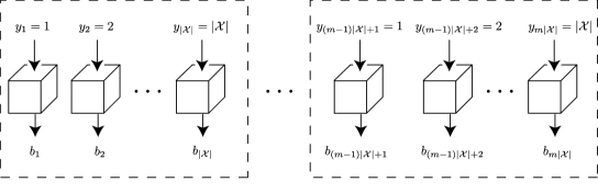
Figure 1: Since $n=m|\mathcal{X}|$, we can divide the particles into $m$ groups of $|\mathcal{X}|$ particles. In each of these groups we measure one particle according to each measurement in $X$ in advance and record a list of all the results. In the simulation, if particle $i$ is supposed to be measured according to a measurement $x\in X$, we just look through the $i$th group until we come to the particle on which measurement $x$ was performed in advance, and output the result we find.

We now provide the formal proof. We construct a separable conditional distribution $Q[A^{m}|X^{m}]$ and then show that it is equal to $P[A^{m}|X^{m}]$. We assume that $\mathcal{X}=\{1,2,\ldots,|\mathcal{X}|\}$, define a vector $y^{n}=(y_{j})_{j=1,\ldots,n}$ with coordinates $y_{j}=(j-1\mod|\mathcal{X}|)+1$, and define the separable state

$$Q[A^{m}|X^{m}]=\sum_{b^{n}}q_{b^{n}}Q_{b^{n},1}[A_{1}|X_{1}]\cdots Q_{b^{n},m}[A_{m}|X_{m}],$$

where $b^{n}\in A^{n}$ is distributed according to $q_{b^{n}}=P[A^{n}=b^{n}|X^{n}=y^{n}]$ and the single-particle conditional probability distributions are deterministic and defined by $Q_{b^{n},i}[A_{i}=a_{i}|X_{i}=x_{i}]=[a_{i}=b_{(i-1)|\mathcal{X}|+x_{i}}]$, where $[t]=1$ if $t$ is true and $0$ otherwise. Let $\mathcal{L}=\{1,2,\ldots,n\}$, $\mathcal{L}_{1}=\{(i-1)|\mathcal{X}|+x_{i}:i=1,2,\ldots,m\}$ and $\mathcal{L}_{2}=\mathcal{L}\backslash\mathcal{L}_{1}$. Further let $A^{\mathcal{L}}=A^{n}$, $A^{\mathcal{L}_{1}}=(A_{x_{1}},A_{|\mathcal{X}|+x_{2}},\ldots,A_{(m-1)|\mathcal{X}|+x_{m}})$ and $A^{\mathcal{L}_{2}}=A^{\mathcal{L}}\backslash A^{\mathcal{L}_{1}}$ and define $b^{\mathcal{L}},b^{\mathcal{L}_{1}}$ and $b^{\mathcal{L}_{2}}$ similarly. We find

$$Q [A^{m}=a^{m}|X^{m}=x^{m}]$$

$$=\sum_{b^{n}}P[A^{n}=b^{n}|X^{n}=y^{n}][a_{1}=b_{x_{1}}]\cdots[a_{m}=b_{(m-1)|\mathcal{X}|+x_{m}}]$$

$$=\sum_{b^{\mathcal{L}_{2}}}P[A^{\mathcal{L}_{1}}=a^{m},A^{\mathcal{L}_{2}}=b^{\mathcal{L}_{2}}|X^{\mathcal{L}_{1}}=x^{m},X^{\mathcal{L}_{2}}=y^{\mathcal{L}_{2}}]$$

$$=P[A^{\mathcal{L}_{1}}=a^{m}|X^{\mathcal{L}_{1}}=x^{m}]=P[A^{m}=a^{m}|X^{m}=x^{m}],$$

where we started with the definition of $Q[A^{m}|X^{m}]$, split the summation over $\mathcal{L}_{1}$ and $\mathcal{L}_{2}$, dropped the conditioning over $X^{\mathcal{L}_{2}}=y^{\mathcal{L}_{2}}$ because of the no-signalling property of $P$, used the definition of a marginal state, and, lastly, the permutation-invariance of $P$. ∎

Our next statement is a de Finetti theorem for symmetric separable conditional probability distributions.

Lemma 5.

Suppose that $P[A^{m}|X^{m}]$ is a symmetric separable conditional probability distribution. Then there exists a probability distribution $p_{\lambda}$ such that

$$\begin{split}\bigl{\|}P[A^{k}|X^{k}]-&\sum_{\lambda}p_{\lambda}P_{\lambda}[A|X]^{\times k}\bigr{\|}\leq\min\biggl{(}\frac{2k|\mathcal{A}|^{|\mathcal{X}|}}{m},\frac{k(k-1)}{m}\biggr{)},\end{split}$$ (9)

where $p_{\lambda}$ is a probability distribution on a finite set of conditional probability distributions, labeled by $\lambda$.

Proof.

Let $Q_{1}[A|X],\ldots,Q_{E}[A|X]$ be the extreme points of the set of conditional probability distributions of one system. These are the deterministic functions $\mathcal{X}\mapsto\mathcal{A}$, hence $E=|\mathcal{A}|^{|\mathcal{X}|}$. Any symmetric separable conditional probability distribution is a convex combination of conditional probability distributions of the form $Q[A^{m}|X^{m}]=\frac{1}{m!}\sum_{\pi}Q_{i_{\pi^{-1}(1)}}[A|X]\cdots Q_{i_{\pi^{-1}(m)}}[A|X]$, where $1\leq i_{1},\ldots,i_{m}\leq E$. Define $Q[A|X]\mathrel{\mathop{:}}=\frac{1}{m}\sum_{j=1}^{m}Q_{i_{j}}[A|X]$. We expand

$$Q[A|X]^{\times k}=\sum_{j_{1}=1}^{m}\cdots\sum_{j_{k}=1}^{m}M_{m}(i_{j_{1}},\ldots,i_{j_{k}})Q_{i_{j_{1}}}[A_{1}|X_{1}]\cdots Q_{i_{j_{k}}}[A_{m}|X_{m}],$$ (10)

where $M_{m}(i_{j_{1}},\ldots,i_{j_{k}})=1/m^{k}$ is the multinomial distribution. To compare this expression with $Q[A^{k}|X^{k}]$, write

$$Q[A^{k}|X^{k}]=\sum_{j_{1}=1}^{m}\cdots\sum_{j_{k}=1}^{m}H_{m}(i_{j_{1}},\ldots,i_{j_{k}})Q_{i_{j_{1}}}[A_{1}|X_{1}]\cdots Q_{i_{j_{k}}}[A_{m}|X_{m}],$$ (11)

where $H_{m}(i_{j_{1}},\ldots,i_{j_{k}})$ is the hypergeometric distribution for an urn with $m$ balls (see Diaconis and Freedman (1980)). Then

$$\left\|Q[A^{k}|X^{k}]-Q[A|X]^{\times k}\right\| =\big{\|}\sum_{j_{1},\ldots,j_{k}}\big{(}H_{m}(i_{j_{1}},\ldots,i_{j_{k}})$$

$$\qquad M_{m}(i_{j_{1}},\ldots,i_{j_{k}})\big{)}Q_{i_{j_{1}}}[A_{1}|X_{1}]\cdots Q_{i_{j_{k}}}[A_{m}|X_{m}]\big{\|}$$

$$\leq\sum_{j_{1},\ldots,j_{k}}\big{|}H_{m}(i_{j_{1}},\ldots,i_{j_{k}})-M_{m}(i_{j_{1}},\ldots,i_{j_{k}})\big{|}$$

$$\leq\min\left(\frac{2kE}{m},\frac{k(k-1)}{m}\right),$$ (12)

where we used the triangle inequality and Diaconis and Freedman’s result on estimating the hypergeometric distribution with a multinomial distribution Diaconis and Freedman (1980). ∎

These two lemmas enable the proof of Theorem 3.

Proof of Theorem 3.

Set $m=\lceil n/|\mathcal{X}|\rceil$ and apply Lemma 4. Then apply Lemma 5. ∎

Our final result is an application to quantum theory. In complete analogy to Lemma 5 we show that the $k$-particle reduced state of a every separable symmetric density operator on $m$ copies of $\mathbb{C}^{d}$ is approximated by a convex combination of tensor product states. Importantly, the approximation guarantee is independent of the dimension $d$, in contrast to the case of entangled states where a dependence on the dimension is necessary Christandl et al. (2007). The norm is given by the trace norm $||A||_{1}=\mathsf{Tr}\sqrt{A^{\dagger}A}$ for operators $A$ on $\mathbb{C}^{d}$. It induces a distance measure on the set of quantum states that has a similar interpretation as a measure of distinguishability as the variational distance for probability distributions and the trace distance introduced on conditional probability distributions.

Theorem 6.

If $\rho$ is a separable permutation-invariant density operator on $(\mathbb{C}^{d})^{\otimes n}$, then there is a measure $m(\sigma)$ on states $\sigma$ on $\mathbb{C}^{d}$ such that

$$\bigl{\|}\rho^{k}-\int dm(\sigma)\,\sigma^{\otimes k}\bigr{\|}_{1}\leq 2\frac{k(k-1)}{n}.$$ (13)

Proof.

Any symmetric separable state is a convex combination of states of the form $\omega^{n}=\frac{1}{n!}\sum_{\pi}\tau_{{\pi^{-1}(1)}}\otimes\cdots\otimes\tau_{{\pi^{-1}(n)}}$, where $\{\tau_{j}\}_{j=1}^{n}$ is a set of pure states (these are extreme points in $\mathcal{B}(\mathbb{C}^{d})$). Define $\tau\mathrel{\mathop{:}}=\frac{1}{n}\sum_{j=1}^{n}\tau_{j}$. We expand

$$\tau^{\otimes k}=\sum_{j_{1}=1}^{n}\cdots\sum_{j_{k}=1}^{n}M_{n}({j_{1}},\ldots,{j_{k}})\tau_{{j_{1}}}\otimes\cdots\otimes\tau_{{j_{k}}},$$ (14)

where $M_{n}({j_{1}},\ldots,{j_{k}})=1/n^{k}$ is the multinomial distribution. To compare this expression with $\omega^{k}:=\mathsf{Tr}_{n-k}\omega^{n}$, write

$$\omega^{k}=\sum_{j_{1}=1}^{n}\cdots\sum_{j_{k}=1}^{n}H_{n}({j_{1}},\ldots,{j_{k}})\tau_{{j_{1}}}\otimes\cdots\otimes\tau_{{j_{k}}},$$ (15)

where $H_{n}({j_{1}},\ldots,{j_{k}})$ is the hypergeometric distribution for an urn with $n$ balls (see Diaconis and Freedman (1980)). Then

$$\left\|\omega^{k}-\tau^{\otimes k}\right\|_{1} =\big{\|}\sum_{j_{1},\ldots,j_{k}}\big{(}H_{n}({j_{1}},\ldots,{j_{k}})$$

$$\qquad M_{n}({j_{1}},\ldots,{j_{k}})\big{)}\tau_{{j_{1}}}\otimes\cdots\otimes\tau_{{j_{k}}}\big{\|}_{1}$$

$$\leq\sum_{j_{1},\ldots,j_{k}}\big{|}H_{n}({j_{1}},\ldots,{j_{k}})-M_{n}({j_{1}},\ldots,{j_{k}})\big{|}$$

$$\leq\frac{k(k-1)}{n},$$ (16)

where we used the triangle inequality and Diaconis and Freedman’s result on estimating the hypergeometric distribution with a multinomial distribution Diaconis and Freedman (1980). ∎

IV Towards a finite de Finetti theorem for the convex sets framework

We will start this section with a self-contained introduction to the convex sets framework. (See Refs. Barnum et al. (2006) and Barnum et al. (2007) for a gentler introduction.) We will then generalise Lemma 5 to this setting. Finally, we pose the question of the existence of a finite de Finetti theorem in the convex sets framework.

Let $\Omega$ be the set of states of a particle. We assume that $\Omega$ is convex, compact, and has affine dimension $n$. In probability theory, for example, $\Omega$ is the simplex of probability distributions $(\omega_{1},\ldots,\omega_{n+1})$, $\omega_{i}\geq 0,\sum_{i}\omega_{i}=1$, while in quantum theory, $\Omega$ is (isomorphic to) the set of positive operators $\omega$ with trace one on a Hilbert space $\mathcal{H}\cong\mathbb{C}^{d}$. We are particularly interested in the case where $\Omega$ is specified by a set of conditional probability distributions $\{P_{\lambda}[A|X]\}$, whose elements are indexed by a label $\lambda$. This is partly because quantum states can be described in this way. For instance, the state $\rho$ of a qubit, a spin-$\frac{1}{2}$ system, is uniquely determined by the probabilities of obtaining spin up or down when it is measured along the $x$, $y$, or $z$ axes of the Bloch sphere. Thus a qubit can be described by a conditional probability distribution $P[A|X]$ with $\mathcal{A}=\{\uparrow,\downarrow\}$ and $\mathcal{X}=\{x,y,z\}$. Not all conditional probability distributions can be obtained by making local measurements on quantum states. This led Barrett to define generalized theories Barrett (2007), where the state space $\Omega$ is the set of all conditional probability distributions $\{P_{\lambda}[A|X]\}$, denoted $\square$. This is the case that we considered in the previous parts of the paper. When $|\mathcal{X}|=1$, this reduces to classical probability theory. In quantum theory, $|\mathcal{X}|=1$ corresponds to the case where all measurements on a system commute, and thus can be performed at once. In fact, every $\Omega$ can be mapped to a convex subset of $\square$ for some number of fiducial measurements and outcomes (Barnum et al., 2006, Lemma 1).

In quantum theory, the most general measurement that can be performed is a positive operator-valued measure (POVM), whose elements are termed effects. Effects are linear functions mapping states to probabilities: in (finite-dimensional) quantum theory, the probability of obtaining the outcome associated with an effect $r$, when the state is $\omega$, is $r(\omega)=\mathsf{Tr}\left(R\omega\right)$ for some bounded nonnegative operator $R$ with $R\leq\mathbf{1}$. In a generalized theory, effects are also functions mapping states to probabilities, and these functions should be affine so that they are compatible with preparing convex combinations. The vector space of affine functions $a:\Omega\to\mathbb{R}$, denoted $A(\Omega)$, is isomorphic to $\mathbb{R}^{n+1}$. The cone of nonnegative affine functions on $\Omega$ is denoted $A_{+}(\Omega)$. The order unit of $A(\Omega)$ is the element $e\in A(\Omega)$ satisfying $e(\omega)=1$ for all $\omega\in\Omega$. An effect is an element $a\in A(\Omega)$ satisfying $0\leq a(\omega)\leq 1$ for all $\omega\in\Omega$. The set of all effects is denoted $[0,e]$. There is a natural embedding of $\Omega$ into $A(\Omega)^{*}$, the dual space of $A(\Omega)$, given by $\omega\mapsto\hat{\omega}$, where $\hat{\omega}(a)=a(\omega)$ for all $a\in A(\Omega)$. Furthermore, if $\hat{\omega}\in A(\Omega)^{*}$ satisfies $\hat{\omega}(a)\geq 0$ for all $a\in A_{+}(\Omega)$ and $\hat{\omega}(e)=1$, then $\hat{\omega}$ is the image of some state $\omega\in\Omega$ (Boyd and Vandenberghe, 2004, Section 2.6). We identify $\hat{\omega}$ with $\omega$ in what follows. It is easy to check that $\|\cdot\|\>=\sup_{a\in[0,e]}|a(\cdot)|$ is a norm on $A(\Omega)^{*}$. For more details about the convex sets framework, see Barnum et al. (2006, 2007).

A natural distance measure on the set of states, which generalises the variational distance between classical probability distributions and the trace distance between quantum states, is given by

$$\|\omega-\omega^{\prime}\|\>=\sup_{a\in[0,e]}|a(\omega)-a(\omega^{\prime})|.$$ (17)

In quantum theory, systems are combined by taking the tensor product of the Hilbert spaces for each system. The same is true in the convex sets framework: $\omega\otimes\omega^{\prime}$ is defined to be the product state where system $\Omega$ is in state $\omega$, system $\Omega^{\prime}$ is in state $\omega^{\prime}$, and the two systems are independent. The complication is that the space $A(\Omega)^{\star}$ is a Banach space but not a Hilbert space and there are multiple ways to define a norm on the tensor product space, consistent with the norm on $A(\Omega)^{\star}$. This choice affects the set of pure (i.e., norm $1$) states of the joint system. At the very least, we want the set of joint states to be closed under convex combinations. This yields:

Definition 7.

The minimal tensor product of $\Omega$ and $\Omega^{\prime}$, denoted by $\Omega\otimes_{\text{min}}\Omega^{\prime}$ consists of all convex combinations of product states $\omega\otimes\omega^{\prime}$, $\omega\in\Omega$ and $\omega^{\prime}\in\Omega^{\prime}$.

We say that states in $\Omega\otimes_{\text{min}}\Omega^{\prime}$ are separable, thereby extending terminology from quantum mechanics to the convex sets framework. Next, if $a$ is a valid effect for system $\Omega$ and $a^{\prime}$ a valid effect for system $\Omega^{\prime}$, then $a\otimes a^{\prime}$ is the effect defined on product states via $a\otimes a^{\prime}(\omega\otimes\omega^{\prime})=a(\omega)a^{\prime}(\omega^{\prime})$. If all convex combinations of such effects are to be allowed, the state space must only contain states in the maximal tensor product, defined via duality as:

Definition 8.

The maximal tensor product of $\Omega$ and $\Omega^{\prime}$, denoted by $\Omega\otimes_{\text{max}}\Omega^{\prime}$ consists of all bilinear functions $\mu:A(\Omega)\times A(\Omega^{\prime})\rightarrow\mathbb{R}$ that satisfy $\mu(a\otimes b)\geq 0$ for $a,b\geq 0$, and $\mu(e\otimes e^{\prime})=1$.

Thus $\mu\in\Omega\otimes_{\text{max}}\Omega^{\prime}$ can be written as a linear combination of product states, possibly with negative weights. In classical probability theory, the minimal and the maximal tensor product coincide. In general, a tensor product $\Omega\otimes\Omega^{\prime}$ is a convex set with $\Omega\otimes_{\text{min}}\Omega^{\prime}\subseteq\Omega\otimes\Omega^{\prime}\subseteq\Omega\otimes_{\text{max}}\Omega^{\prime}$. In quantum theory, $\Omega\otimes\Omega^{\prime}$ is the set of trace one positive operators on the (unique) Hilbert space tensor product of $\mathcal{H}$ and $\mathcal{H}^{\prime}$. Note that $\Omega\otimes\Omega^{\prime}$ lies strictly between the maximal and minimal tensor products in the quantum case. The set of separable quantum states is $\Omega\otimes_{\text{min}}\Omega^{\prime}$ and $\Omega\otimes_{\text{max}}\Omega^{\prime}$ is the set of trace one entanglement witnesses.

For a state $\mu\in\Omega\otimes\Omega^{\prime}$, we say that $\mu_{\Omega}\in\Omega$, defined by $a(\mu_{\Omega})=a\otimes e^{\prime}(\mu)$ for all effects $a$, is the partial trace of $\mu$ with respect to $\Omega^{\prime}$. An effect on the tensor product is an element $a\in A(\Omega\otimes\Omega^{\prime})$ satisfying $0\leq a\leq e\otimes e^{\prime}$. The larger the set of joint states, the smaller the set of allowed effects. This means that the distance measure that we defined in Eq. (17), when applied to states of more than one particle, depends on which tensor product we use. It is true, however, that $\|\omega-\omega^{\prime}\|\leq\|\omega-\omega^{\prime}\|_{\text{min}}$, the distance measure for the minimal tensor product, since in that case the set of effects is largest. Also note that a physical theory may place additional restrictions on which effects are allowed but, even then, $\|\omega-\omega^{\prime}\|$ provides an upper bound on the probability of distinguishing $\omega$ and $\omega^{\prime}$.

Theorem 9.

Let $\Omega$ be a convex set with $E$ extreme points ($E$ may be infinite). Suppose $\omega^{n}\in\Omega^{\otimes_{\text{min}}n}$ is symmetric. Then there is a measure $m(\tau)$ on states $\tau\in\Omega$ such that

$$\bigl{\|}\omega^{k}-\int dm(\tau)\,\tau^{\otimes k}\bigr{\|}_{\text{min}}\leq\min\left(\frac{2kE}{n},\frac{k(k-1)}{n}\right).$$ (18)

Proof.

Let $\tau_{1},\ldots,\tau_{E}$ be the extreme points of $\Omega$. Any symmetric separable state is a convex combination of states of the form $\omega^{n}=\frac{1}{n!}\sum_{\pi}\tau_{i_{\pi^{-1}(1)}}\otimes\cdots\otimes\tau_{i_{\pi^{-1}(n)}}$, where $1\leq i_{1},\ldots,i_{n}\leq E$. Define $\tau\mathrel{\mathop{:}}=\frac{1}{n}\sum_{j=1}^{n}\tau_{i_{j}}$. We expand

$$\tau^{\otimes k}=\sum_{j_{1}=1}^{n}\cdots\sum_{j_{k}=1}^{n}M_{n}(i_{j_{1}},\ldots,i_{j_{k}})\tau_{i_{j_{1}}}\otimes\cdots\otimes\tau_{i_{j_{k}}},$$ (19)

where $M_{n}(i_{j_{1}},\ldots,i_{j_{k}})=1/n^{k}$ is the multinomial distribution. To compare this expression with $\omega^{k}$, write

$$\omega^{k}=\sum_{j_{1}=1}^{n}\cdots\sum_{j_{k}=1}^{n}H_{n}(i_{j_{1}},\ldots,i_{j_{k}})\tau_{i_{j_{1}}}\otimes\cdots\otimes\tau_{i_{j_{k}}},$$ (20)

where $H_{n}(i_{j_{1}},\ldots,i_{j_{k}})$ is the hypergeometric distribution for an urn with $n$ balls (see Diaconis and Freedman (1980)). Then

$$\left\|\omega^{k}-\tau^{\otimes k}\right\|_{\text{min}} =\big{\|}\sum_{j_{1},\ldots,j_{k}}\big{(}H_{n}(i_{j_{1}},\ldots,i_{j_{k}})$$

$$\qquad M_{n}(i_{j_{1}},\ldots,i_{j_{k}})\big{)}\tau_{i_{j_{1}}}\otimes\cdots\otimes\tau_{i_{j_{k}}}\big{\|}_{\text{min}}$$

$$\leq\sum_{j_{1},\ldots,j_{k}}\big{|}H_{n}(i_{j_{1}},\ldots,i_{j_{k}})-M_{n}(i_{j_{1}},\ldots,i_{j_{k}})\big{|}$$

$$\leq\min\left(\frac{2kE}{n},\frac{k(k-1)}{n}\right),$$ (21)

where we used the triangle inequality and Diaconis and Freedman’s result on estimating the hypergeometric distribution with a multinomial distribution Diaconis and Freedman (1980). ∎

One can show that $\square^{\otimes_{\text{max}}n}$ is precisely the set of all no-signalling conditional probability distributions and that $\square^{\otimes_{\text{min}}n}$ is the set of all separable conditional probability distributions  Randall and Foulis (1981); Barrett (2007). Furthermore the trace distance (Definition 2) coincides with the definition in Eq. (17). With these observations and the fact that $||\cdot||\leq||\cdot||_{\min}$ we see that Theorem 9 generalises Lemma 5. Unfortunately, we were not able to obtain a similar generalisation of Lemma 4 and hence of Theorem 3. We thus conclude with the question of whether a finite de Finetti theorem exists for general theories in the convex sets framework. We remark that the argument of Caves et al. (2002) applied in this context yields an infinite de Finetti theorem for any theory in the convex sets framework (see Barrett and Leifer (2007) for the details).

V Acknowledgements

This work was carried out at the same time as related work by J. Barrett and M. Leifer Barrett and Leifer (2007). We thank them for discussions, and especially for explaining how to define the trace distance. We thank R. Colbeck and R. Renner for discussions, G. Mitchison for valuable comments on the manuscript, and the organizers of the FQXi workshop Operational probabilistic theories as foils to quantum theory, where part of this work was done. MC thanks the IQI at Caltech and CWI Amsterdam for their hospitality. This work was supported by the UK’s EPSRC, Magdalene College Cambridge, NSF Grants PHY-0456720 and CCF-0524828, EU Projects SCALA (CT-015714) and QAP (CT-015848), NWO VICI project 639-023-302, and the Dutch BSIK/BRICKS project.

References

- Diaconis and Freedman (1980) P. Diaconis and D. Freedman, Ann. Probab. 8, 745 (1980).
- Bernardo and Smith (1994) J. M. Bernardo and A. F. M. Smith, Bayesian Theory (Wiley, Chichester, 1994).
- de Finetti (1937) B. de Finetti, Ann. Inst. H. Poincaré 7, 1 (1937).
- König and Renner (2005) R. König and R. Renner, J. Math. Phys. 46, 122108 (2005), quant-ph/0410229.
- Christandl et al. (2007) M. Christandl, R. König, G. Mitchison, and R. Renner, Comm. Math. Phys. 273, 473 (2007), quant-ph/0602130.
- Renner (2005) R. Renner, Ph.D. thesis, Swiss Federal Institute of Technology, Zürich (2005), quant-ph/0512258; Nature Physics 3, 645 (2007), quant-ph/0703069.
- Bennett and Brassard (1984) C. H. Bennett and G. Brassard, in Proceedings of IEEE International Conference on Computers, Systems, and Signal Processing (IEEE, 1984), pp. 175–179; A. K. Ekert, Phys. Rev. Lett. 67, 661 (1991).
- Acín et al. (2007) A. Acín, N. Brunner, N. Gisin, S. Massar, S. Pironio, and V. Scarani, Phys. Rev. Lett. 98, 230501 (2007), quant-ph/0702152; J. Barrett, L. Hardy, and A. Kent, Phys. Rev. Lett. 95, 010503 (2005), quant-ph/0405101; Ll. Masanes, R. Renner, A. Winter, J. Barrett and M. Christandl, quant-ph/0606049; A. Acín, N. Gisin, and Ll. Masanes, Phys. Rev. Lett. 97, 120405 (2006), quant-ph/0510094; V. Scarani, N. Gisin, N. Brunner, Ll. Masanes, S. Pino, and A. Acín, Phys. Rev. A 74, 042339 (2006), quant-ph/0606197.
- Caves et al. (2002) C. M. Caves, C. A. Fuchs, and R. Schack, J. Math. Phys. 43, 4537 (2002), quant-ph/0104088.
- Barnum et al. (2006) H. Barnum, J. Barrett, M. Leifer, and A. Wilce (2007), quant-ph/0611295.
- Barnum et al. (2007) H. Barnum, J. Barrett, M. Leifer, and A. Wilce, Phys. Rev. Lett. 99, 240501 (2007), arXiv:0707.0620.
- Barrett and Leifer (2007) J. Barrett and M. Leifer (2007), arXiv:0712.2265.
- Størmer (1969) E. Størmer, J. Funct. Anal. 3, 48 (1969); R. L. Hudson and G. R. Moody, Z. Wahrschein. verw. Geb. (Probab. Theory Related Fields) 33, 343 (1976).
- Fuchs et al. (2004) C. A. Fuchs, R. Schack, and P. F. Scudo, Phys. Rev. A 69, 062305 (2004), quant-ph/0307198.
- Christandl and Toner (2009) M. Christandl and B. Toner (2009), in preparation.
- Eggeling and Werner (2002) T. Eggeling and R. Werner, Phys. Rev. Lett. 89, 097905 (2002).
- Hayden et al. (2005) P. Hayden, D. Leung, and G. Smith, Phys. Rev. A 71, 062339 (2005).
- Barrett (2007) J. Barrett, Phys. Rev. A 75, 032304 (2007), quant-ph/0508211.
- Werner (1989) R. F. Werner, Lett. Math. Phys. 17, 359 (1989); B. M. Terhal, A. C. Doherty, and D. Schwab, Phys. Rev. Lett. 90, 157903 (2003), quant-ph/0210053; B. F. Toner, Proc. R. Soc. A 465, 59–69 (2009), quant-ph/0601172.
- Boyd and Vandenberghe (2004) S. Boyd and L. Vandenberghe, Convex Optimization (Cambridge University Press, Cambridge, 2004), available online at http://www.stanford.edu/~boyd/cvxbook/.
- Randall and Foulis (1981) C. H. Randall and D. J. Foulis, in Interpretations and Foundations of Quantum Mechanics, edited by H. Neumann (Bibliographisches Institut, Wissenschaftsverlag, Manheim, 1981).
- Popescu and Rohrlich (1994) S. Popescu and D. Rohrlich, Found. Phys. 24, 379 (1994).