A mean-field model for the electron glass dynamics

Abstract

We study a microscopic mean-field model for the dynamics of the electron glass, near a local equilibrium state. Phonon-induced tunneling processes are responsible for generating transitions between localized electronic sites, which eventually lead to the thermalization of the system. We find that the decay of an excited state to a locally stable state is far from being exponential in time, and does not have a characteristic time scale. Working in a mean-field approximation, we write rate equations for the average occupation numbers $\langle n_{i}\rangle$, and describe the return to the locally stable state using the eigenvalues of a rate matrix, $A$, describing the linearized time-evolution of the occupation numbers. Analyzing the probability distribution $P(\lambda)$ of the eigenvalues of $A$ we find that, under certain physically reasonable assumptions, it takes the form $P(\lambda)\sim\frac{1}{|\lambda|}$, leading naturally to a logarithmic decay in time. While our derivation of the matrix $A$ is specific for the chosen model, we expect that other glassy systems, with different microscopic characteristics, will be described by random rate matrices belonging to the same universality class of $A$. Namely, the rate matrix has elements with a very broad distribution, i.e., exponentials of a variable with nearly uniform distribution.

I Introduction

Experiments conducted on thin-films of amorphous or crystalline semiconductors such as indium-oxide or silicon, show that when driven out-of-equilibrium (for example by shining light on the system or by changing a gate voltage), the system exhibits slow relaxations, observable on the scale of minutes or hours monroe1 ; Zvi:1 . In many cases a logarithmic or weak power-law time-dependence of the measured quantity (such as conductance and capacitance) is observed over many decades of time Martinez ; Zvi:5 ; silicon_glass . A common feature of the experimental systems is that they are highly disordered, so that most electronic states are localized. If the carrier concentration is high enough condition_of_high_density , the (unscreened) Coulomb interactions may play an important role Zvi:2 . This system is usually referred to as the electron glass, since it exhibits many features characteristic of glassy systems: memory effects  Zvi:4 (the conductance depends on the previous perturbations applied to the system) and aging Zvi:3 (the duration of time of the perturbation is applied affects the relaxation timescales). Similar effects have been observed in granular Al grenet1 ; grenet2 showing that the underlying principles may be more general.

In this paper we study a mean-field model for the dynamics of the system. A variety of systems in nature can be described, near a locally stable state, by a matrix equation of the type:

$$\frac{d\vec{\delta n}}{dt}=A\cdot\vec{\delta n},$$ (1)

the component $\delta n_{i}=n_{i}-f_{i}$ is the deviation of the average occupation of the i’th site, $n_{i}$, from its value $f_{i}$ at the locally stable point. The local stability of the point implies that the matrix $A$ must have only non-positive eigenvalues, and, for large systems, their distribution will determine the average time-dependence of the return to the locally stable point, after the system was slightly pushed away from it. It must be emphasized that our approach is different from the usual theoretical explanations of aging phenomena in glasses, in which the system explores the energy landscape, and slow relaxations are a result of the existence of many metastable states. In our model, the system is found in the vicinity of one locally stable point, at all times (we do not use the term metastable to stress this difference). This assumes that the initial perturbation is small enough (and so is the temperature), such the system does not reach other (lower) minima, but remains in the same region of phase space. Slow relaxations are due to isolated states that, statistically, happen to have a long life time. It should be emphasized that although the interactions lead to the non-trivial Coulomb gap efros in the equilibrium state, the slow dynamics will occur also without interactions.

If it is given that the distribution of eigenvalues diverges at small (negative) eigenvalues, and is of the form $P(\lambda)\sim\frac{1}{|\lambda|}$ (as happens in our model) it is straightforward to see that logarithmic relaxation in time, in an appropriate time window, is obtained (assuming the eigenvectors are excited with uniform probability). In this work we show that starting from a realistic microscopic model for the electron glass system, the described situation indeed occurs, and we argue that it is plausible that other physical systems will also show similar results.

The structure of the paper is as follows. The model is defined in II.1. In II.2, we review the application of the mean-field approximation to the peculiar equilibrium properties of the system, manifesting the Coulomb gap. In II.3, we briefly discuss the mean-field steady-state solution in the presence of an external field, leading to the Miller-Abrahams model miller_abrahams .

In a similar fashion, in section III we suggest to study the dynamics of the system by writing a set of ordinary differential equations, described by Eqs. (2) and (6), giving the time-evolution of the occupancies of the localized states. This is already an approximation neglecting interference or quantum fluctuation effects. In III.1, we study the dynamics of the electron glass, starting from an out-of-equilibrium state. Linearizing Eq. (2), we obtain the time-evolution equations of the occupations and obtain Eq. (1), with the random matrix $A$ belonging to a different class from the usual gaussian random matrix ensembles. The statistics of the eigenvalues is studied numerically, see Fig. 3. In III.2 we study a simplifying limit, analytically. Both lead to a distribution of eigenvalues $P(\lambda)$ diverging at low values (down to a cutoff), leading to slow relaxations of the physical observables, as seen experimentally. This behaviour might be characteristic of glassy systems. Finally, in III.3, we discuss the relation between the relaxation of the occupation numbers and the conductance.

II Mean-field model for electron glass

In this section we discuss a specific microscopic model for the dynamics of the electron glass. We will show that it leads to a rate equation of the type of Eq. (1), and find explicitly the matrix elements.

II.1 Definition of the model

We study a system of $N$ localized states and $M<N$ electrons, with a coupling between the electrons and a phonon reservoir. Since the states are localized, the electrons will interact via an unscreened Coulomb potential. In the absence of electron-electron interactions, the localized states have different energies, $\epsilon_{i}$, due to the disorder. Our model also contains structural disorder: the positions of the sites are assumed to be random. Although localized states are orthogonal, their tails overlap, and therefore phonons may induce transitions between them. The generic coupling between electrons and phonons is given by the form $\sum_{q}M_{q}c_{i}^{{\dagger}}c_{j}(b^{{\dagger}}_{q}+b_{-q})$ where $c_{i}^{{\dagger}},c_{j}$ are electron creation and annihilation operators at local sites $i,j$ and $b_{q}$ annihilates a phonon. $M_{q}$ is a coefficient accounting for the strength of the electron-phonon coupling.

Let us denote the energy difference of the electronic system before and after the tunneling event by $\Delta E$, containing the interaction effects. For weak electron-phonon coupling ($|M_{q}|^{2}\nu\ll\Delta E$, where $\nu$ is the phonon density of states), the transition rate $\gamma_{ij}$ of an electron from site $i$ with energy $E_{i}$ to site $j$ with energy $E_{j}<E_{i}$ a distance $r_{ij}$ away, can be calculated treating the coupling as a perturbation. This yields, up to polynomial corrections efros :

$$\gamma_{ij}\sim|M_{q}|^{2}\nu f_{i}(1-f_{j})e^{-\frac{r_{ij}}{\xi}}[1+N(\Delta E)],$$ (2)

where $f_{i}$ is the Fermi-Dirac distribution. For upward transitions ($E_{j}>E_{i}$) the square brackets are replaced by $N(\Delta E)$. These rates may be renormalized due to polaron-type orthogonality effects leggett_review .

We will be interested in the dynamics of the system when it is out-of-equilibrium, namely in the time-dependence of the occupation numbers and the conductance after an initial excitation. But we first show how non-trivial equilibrium properties are obtained from the mean-field picture.

II.2 Equilibrium properties near a locally stable point

In an approximation similar to those used in spin glass theory spin_glass , we define $f_{i}=\langle n_{i}\rangle$, where $n_{i}$ the site occupation (which takes the values zero or one) and $\langle\rangle$ denotes averaging over a time scale much larger than that related to the frequency of the phonon processes but smaller than the relevant scale for the observation of the dynamics. This is a mean-field type approximation, and may be used regardless of the interactions in the system. Let us first discuss the thermal equilibrium state, near the locally stable point. The sites occupation must follow the Fermi-Dirac distribution and therefore:

$$f_{i}(E_{i})=\frac{1}{1+e^{\frac{E_{i}-\mu}{T}}},$$ (3)

where $\mu$ is the chemical potential, and the Boltzmann constant is set to be one.

In the mean-field approximation we can calculate the average potential energy of site $i$:

$$E_{i}=\epsilon_{i}+\sum_{j\neq i}\frac{e^{2}f_{j}}{r_{ij}}.$$ (4)

This approximation improves as the number of interacting sites increases mean_field_infinite . The long range nature of the interaction means that the energy of a site will be determined by many of its neighbours, and gives intuitive justification of the use of mean-field theory. Nevertheless, we should emphasize that this is an uncontrolled approximation, and the limits of its validity should be checked.

Combining Eq. (3) and (4), one obtains a self-consistent equation for the energies. It is common to use an unbiased disorder distribution, and add a background charge $\nu$ to each site coulomb_gap_mean_field . In the mean-field picture, this will lead to the equation:

$$E_{i}=\epsilon_{i}+\sum_{j}\left(\frac{1}{1+e^{\frac{E_{j}-\mu}{T}}}\ -\nu\right)\frac{e^{2}}{r_{ij}}.$$ (5)

For half filling, $\mu=0$, $\nu=0.5$.

One should notice that there are many solutions to this self-consistent equation. Rigorously, one cannot call any solution an equilibrium distribution, since the equilibrium distribution is a Boltzmann average over all configurations, not only those near the locally stable point. The solution may be viewed as a ’local equilibrium’. We will see that the physical picture obtained is quite plausible. At low temperatures T_c , the probability distribution of the energies will contain a soft gap at the Fermi energy, known as the Coulomb gap efros ; efros_sce ; coulomb_gap_mean_field ; peierls ; pankov ; malik ; coulomb_gap_experimental ; coulomb_gap_exp2 .

Eq. (5) can be solved numerically by starting with a random set of energies, and evolving them iteratively, within the mean-field model. This was done following Ref. [coulomb_gap_mean_field, ], by solving the equations for many random instances, and averaging over them. In this way a histogram of the on-site energies is obtained. When normalized correctly, it gives the single-particle DOS (density of states), as function of energy. The results for two-dimensions, yielding the Coulomb gap, are given in Fig. 1. Notice that the obtained DOS contains a linear gap near the Fermi energy, in accordance with other works efros_sce ; coulomb_gap_experimental .

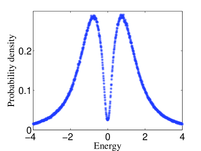
Figure 1: Histogram of the site energies in two dimensions, for N=10000, $\mu=0$ (half filling), obtained by solving the self-consistent Eq. (5). The sites were uniformly distributed in a square, with $\frac{e^{2}}{r_{nn}T}=20$, where $r_{nn}$ denotes the average nearest-neighbor distance and $T$ is the temperature. The energies $\epsilon_{i}$ were uniformly distributed in the interval $[-\frac{W}{2},\frac{W}{2}]$, with $W=1$. The y axis denotes the probability density of the energies $E_{i}$. The graph is the average over 300 instances. Notice the finite value of the density at the minimum, due to the finite temperature.

II.3 Response to an external field: steady-state solution

When a small electric field is applied, there are corrections to the average occupations and also to the average energies. It can be shown that the problem of finding the steady-state solution corresponds to that of solving the steady-state of a resistance network, using Kirchoff’s laws miller_abrahams . The solution, when neglecting interactions, gives the well-known Mott Variable Range Hopping mott , which was observed experimentally in many cases mott_exp . We emphasize that this calculation is in fact a mean-field one: the steady-state solutions are obtained from time-dependent equations which are essentially the mean-field equations. In the following we propose to use the same ideas to discuss the dynamics of the system out-of-equilibrium.

III The Dynamics

Let us pose the following question: How will the occupation numbers or conductance depend on time, when the system is pushed slightly out of the locally stable point? Having seen that the mean-field approximation yields the correct density of states as well as the out-of-equilibrium steady-state solution in the presence of an external field, we propose to use the same approximation to describe the dynamics of the systems, when prepared out of local equilibrium.

Experimentally, the form of the relaxation depends on the details and mechanism of the excitation. For simplicity, let us assume that the initial perturbation takes the form of a random addition $\delta n_{i}$ to the state occupations, with $\sum_{i}\delta n_{i}=0$, reflecting particle number conservation.

Assuming that the initial change in the occupations is small, we can still use Eq. (2) for the tunneling rates, with the average occupations at the locally stable point $f_{j}$ substituted by the occupation numbers slightly out of equilibrium $n_{j}$ (which can take any value between 0 and 1). The energies at each instance are related to the out-of-equilibrium occupations by Eq. (4), upon replacing $f_{j}$ by $n_{j}$, and we can write the time-evolution of the average occupation as:

$$\frac{dn_{i}}{dt}=\sum_{j\neq i}\gamma_{ji}-\gamma_{ij}.$$ (6)

This defines the problem completely. At the locally stable point itself, the RHS of Eq. (6) must vanish. Therefore not too far from the point, we can take the first (linear) order in the quantities $\delta n_{i}$, the deviations from the stable point. The linearized equation then takes the form of Eq. (1), where $\vec{\delta n}$ is a vector of the deviations of the occupation numbers from their local equilibrium values. The $N$ eigenvalues and eigenvectors of the matrix $A$ will determine the decay rates of the system.

We would like to stress that the matrix $A$ can be calculated for the cases of interest, by linearizing the equations of motion near the locally stable point. This strategy is completely general, and will be valid for any system which can be described by equations of motion, and has a locally stable point (such would be the case for most classical systems, and many quantum systems in a mean-field approximation). The dynamics of the system when pushed slightly away from the fixed point, will be characterized by the eigenvalues of the rate matrix. In the common case where disorder plays a role, the dynamics will depend on the distribution of eigenvalues of the matrix, thus, we obtain a problem of random matrix theory mehta , where the eigenvalue distribution is responsible for the dynamics of the system. An extremely relevant property of the electron glass case, as we shall demonstrate in III.1, is that the entries of the random matrix are exponentials of the broadly distributed parameters (energy and distance). Another important feature of these matrices is that the sum of every column vanishes. These properties make this matrix belong to a different class from the usual gaussian ensembles treated in random matrix theory, and will play an important role in the dynamics, leading to slow relaxations. A similar class of matrices was studied previously by Mezard et al. distance_matrices .

In the following section we will derive the form of the matrix $A$ for the particular case of localized states coupled due to phonons. We will find that the probability distribution is divergent for small eigenvalues, and suggest what the minimal properties leading to such a distribution are. The implications of this distribution on the time-dependent relaxation of the occupation numbers and conductance will then be discussed.

III.1 Application to the electron glass model

Starting from Eq. (2), a calculation of the elements of matrix $A$ in Eq. (6) shows that:

$$A_{ii}=\sum_{j\neq i}-\frac{\gamma^{0}_{ij}}{n_{j}(1-n_{j})},$$ (7)

where $\gamma^{0}_{ij}$ are the local equilibrium rates, given by Eq. (2). For $i\neq j$:

$${A_{ij}=\gamma^{0}_{ij}\frac{1}{n_{j}(1-n_{j})}-\sum_{k\neq j,i}\frac{e^{2}\gamma^{0}_{ik}}{T}(\frac{1}{r_{ij}}-\frac{1}{r_{jk}})}.$$ (8)

Notice that the matrix is not symmetric, due to the $n_{j}(1-n_{j})$ term. The sum of each column of the matrix vanishes, guaranteeing particle number conservation.

A-priori one would expect that at low enough temperatures $T\ll\frac{e^{2}}{r_{nn}}$, we could neglect the first term in the equation for the regime of interest. However, at low temperatures the occupations of the sites tend to 0 or 1 exponentially, meaning the $\frac{1}{n_{j}(1-n_{j})}$ term explodes much faster than the $\frac{1}{T}$ part in the second term. Viewed in a different way, if one looks at the expression of the mean-field rates $\gamma_{ij}\sim n_{i}(1-n_{j})[1+N(\Delta E)]$, one sees that if two states are close in energy, then the first term in the matrix element (8) $\sim\frac{n_{i}}{n_{j}}N(\Delta E)\sim\frac{T}{\Delta E}$. Therefore there is good coupling between any two states close in energy (and distance), not only those ones close to the Fermi level, as is the case for the second term. Therefore the ’phase space’ is much larger for the first term, and the second one can be neglected. We have calculated numerically the eigenvalue distribution for some specific system parameters, and indeed it was found that the second part has a small influence on most eigenvalues, see Fig. 2.

An important property follows: the off-diagonal elements are positive. Together with the property that the sum of every column vanishes, the stability of the mean-field solution is guaranteed: all the eigenvalues are negative, characterizing decay. A proof of the statement can be found in Ref. [distance_matrices, ].

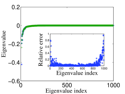
Figure 2: Comparison of the eigenvalues of the full linearized matrix (stars) and the ones obtained after neglecting the ’Coulomb’ term (crosses), the second one in Eq. (8). The difference is mostly seen for the large magnitude eigenvalues. $N=1000$, $\frac{\xi}{r_{nn}}=0.1$ and $\frac{e^{2}}{r_{nn}T}=10$. The energies $\epsilon_{i}$ were uniformly distributed in the interval $[-\frac{W}{2},\frac{W}{2}]$, with $\frac{W}{T}=10$. The inset shows the relative error in replacing the full matrix with the approximated one, defined as the difference between the approximation and exact diagonalization, divided by the exact value.

Let us consider the distribution of the eigenvalues. Fig. 3 shows the distribution of eigenvalues of the matrix $A$, as obtained numerically. We first found a mean-field solution by iterating the equations (see, for example, coulomb_gap_mean_field ), then used Eq. (8) to construct the relevant matrix. The eigenvalues of this matrix were then found numerically. Notice that the localization length $\xi$ influences the dynamics, although it has no effect on the equilibrium properties, at least as long as the localized states are spatially well separated.

In III.2 we will analyze a simplifying limit, when the rather complicated dependence on energy can be neglected, and consider only the exponential dependence of the tunneling rate on length. Both limits give approximately a $\frac{1}{|\lambda|}$ distribution (up to logarithmic corrections), reminiscent of $\frac{1}{f}$ noise 1_f . This suggests that the result may be more general, and not dependent on the details of the specific model. Note that the interactions affect the mean-field solution (and the Coulomb gap), but the calculation shows the slow dynamics will exist also without them.

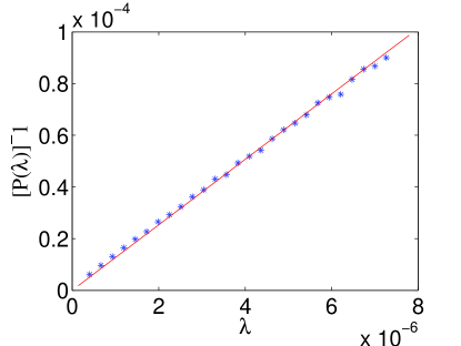
Figure 3: Distribution of eigenvalues obtained numerically, averaged over 1000 realizations. The parameters were as for Fig. 2. The fit to the reciprocal distribution is linear.

Let us now discuss the consequences of this distribution for the dynamics of the system. Having found that the distribution is $\sim\frac{1}{|\lambda|}$ down to some minimal value, we conclude that if all eigenvectors (except the one with eigenvalue zero, not conserving particle number), are excited with equal probability, the time-evolution of the deviation from the local stable point will be related to the Laplace transform of the eigenvalue distribution. This will give rise to logarithmic decays. Let us show this in more detail: if the eigenvectors are denoted by $\vec{n_{\lambda}}$, the time-dependent deviation from the locally stable point will be given by:

$$\vec{\delta n}=\sum_{\lambda}c_{\lambda}\vec{n_{\lambda}}e^{-\lambda t}.$$ (9)

We shall assume the eigenvectors are excited with roughly uniform probability. Going to the continuous limit, and utilizing the fact that the components of the eigenvectors themselves are also random variables, we obtain that the norm of $\vec{\delta n}$ should relax as:

$$|\vec{\delta n}(t)|\sim\int_{\lambda_{min}}^{\lambda_{max}}\frac{e^{-\lambda t}}{\lambda}d\lambda\sim\gamma_{E}-\log[t\lambda_{min}],$$ (10)

for $\frac{1}{\lambda_{min}}<t<\frac{1}{\lambda_{max}}$.

III.2 Dynamics of exponential models

Hitherto we have discussed a specific model for glass dynamics in a system constructed from interacting electrons and phonons. The actual form of the rate matrix eigenvalue distribution did not depend strongly on the details of the matrix elements. In this section we will show that there are few sufficient conditions on the random rate matrix $A$ that will make the relaxation process long.

Let us look at the dynamics which follow from a class of random matrices obeying the following properties:

1. The sum of every column vanishes. This follows from particle number conservation.

2. The entries of the matrices are distributed over a very broad range. This happens, for example, when they are exponentials of a more or less flat distribution pollak .

We expect that a variety of systems that exhibit a glassy behaviour may be described by a random rate matrix belonging to this class. The matrix obtained for the electron glass system indeed obeys these properties. The first property was shown explicitly in section III.1. To see the second, let us examine Eq. (8). If we neglect cases where the energies $E_{i}$, $E_{j}$ and $|E_{i}-E_{j}|$ are smaller than $T$, we can recast the equation into a more transparent form:

$$A_{ij}\sim e^{-\frac{r_{ij}}{\xi}}e^{\frac{-|E_{i}-E_{j}|-|E_{i}|+|E_{j}|}{2T}}.$$ (11)

Due to the exponential, the matrix entries are indeed broadly distributed.

We shall now discuss a specific class of matrices which can be analyzed analytically. As seen in Eq. (11), the matrix elements for the electron glass system contain a factor $e^{\frac{-r_{ij}}{\xi}}$. If $\xi$ is much smaller than the typical distance $r_{nn}$, it is plausible that this factor would be dominant in determining the eigenvalue distribution. This motivates us to discuss a simpler model, of so-called distance matrices distance_matrices : assume we have $N$ random points in a two dimensional space. Let us define a matrix $B_{ij}=e^{-\frac{r_{ij}}{\xi}}$, where $r_{ij}$ is the distance between points $i$ and $j$, and $\xi$ some constant. Let us choose the diagonal elements of the matrix such that the sum of every column vanishes. Following the previous discussion of the dynamics, we are interested in the distribution of eigenvalues of such a matrix. A mapping of this problem to a field theory problem is given in Ref. [distance_matrices, ], enabling one to look at a low-density approximation to the theory. Mezard et. al calculate the resolvent $R=\frac{1}{N}Tr\frac{1}{\lambda-H}$, the imaginary part of which yields the density of states, i.e, the distribution of eigenvalues. Using their formula (21) for the case of $f(r)=e^{-\frac{r}{\xi}}$, we obtain that the low-density expansion of the resolvent is:

$$R(\lambda)=\frac{\rho}{2V}\int dxdy\left(\frac{1}{\lambda+2e^{-\frac{r}{\xi}}}-\frac{1}{\lambda}\right),$$ (12)

where the integrals are performed over the whole volume. The second term gives rise to a delta function at the origin, which comes from the zero eigenvalue the matrix always possesses, and is of no particular interest since the eigenvector associated with this eigenvalue cannot be excited while preserving the particle number. The condition for the approximation to be valid is $\xi\ll r_{nn}$, as we shall show later in a more transparent way.

Since the density of states is given by $-\frac{Im[R(\lambda)]}{\pi}$, we can use the fact that $Im[\frac{1}{x+i\epsilon}]=-i\pi\delta(x)$ and obtain the DOS as:

$$P(\lambda)=\frac{\rho}{2V}\int dxdy\delta(\lambda+2e^{-\frac{r}{\xi}}).$$ (13)

Performing the integral in one-dimension, for eigenvalues not too close to the minimal value $2e^{-\frac{L}{\xi}}$, leads to the result:

$$P(\lambda)=\frac{-N\xi}{L\lambda},$$ (14)

with $\lambda$ in the interval $[-2,-2e^{\frac{-L}{\xi}}]$.

Repeating the calculation in two-dimensions, again, for eigenvalues not too close to the minimal values, yields:

$$P(\lambda)=\frac{\pi N\xi^{2}\log(-\frac{\lambda}{2})}{L^{2}\lambda}.$$ (15)

We shall now give a transparent demonstration of these results. In the low density limit, we can couple each site to its nearest-neighbor, thus dividing the system into $\frac{N}{2}$ pairs. Neglecting the effect of all other sites, we obtain that the eigenvalues will be similar to those of an ensemble of 2X2 matrices of the form:

$$M=\left(\begin{array}[]{cccc}-e^{\frac{-|x-y|}{\xi}}&e^{\frac{-|x-y|}{\xi}}\\ e^{\frac{-|x-y|}{\xi}}&-e^{\frac{-|x-y|}{\xi}}\\ \end{array}\right).$$ (16)

Since the matrix elements of $B$ decay on the scale of $\xi$, this would be a good approximation for $\xi\ll r_{nn}$. One eigenvalue of $M$ is 0, and the other is $-2e^{\frac{-|x-y|}{\xi}}$. Therefore half the eigenvalues of $B$ will be the zero under this approximation, and the distribution of the other eigenvalues will be that of the random variable $-2e^{\frac{-r}{\xi}}$, where $r$ is the nearest-neighbour distance. Notice the zero eigenvalues correspond to the second term in Eq. (12).

The distribution of the nearest-neighbour distance can be calculated: looking at a typical site, let us calculate the probability that its nearest-neighbour is at least distance $r$ away. This is equivalent to asking that all of its neighbours are at least a distance $r$ away, and since they are randomly distributed, we obtain that:

$$Prob(r)=(1-V_{D}\frac{r^{D}}{L^{D}})^{N-1},$$ (17)

where $V_{1}=2$ and $V_{2}=\pi$.

For $r\ll L$ we can approximate:

$$Prob(r)=e^{-V_{D}N\frac{r^{D}}{L^{D}}}.$$ (18)

We have assumed that the initial site is not too close to the boundaries. Since we are interested in the probability, the sites near the boundary will give a negligible correction to the above probability: the sites for which Eq. (18) fails are a distance of order $r_{nn}$ or less from the boundary. Therefore their fraction in the system is of order $\frac{r_{nn}}{L}$. For $N\gg 1$, this fraction is negligible.

The probability distribution can be calculated by differentiating with respect to $r$, leading to:

$$P(r)=V_{d}DN\frac{r^{D-1}}{L^{D}}e^{-V_{D}N\frac{r^{D}}{L^{D}}}.$$ (19)

By construction, the probability distribution is exactly normalized.

In one-dimension, the eigenvalue distribution that follows is:

$$P(\lambda)=-N\frac{e^{\frac{-2N\xi}{L}|\log(-\frac{\lambda}{2})|}}{L\lambda}\xi\sim\frac{1}{\lambda^{1-\epsilon}},$$ (20)

with $\epsilon=\frac{2N\xi}{L}\ll 1$, while for two-dimensions:

$$P(\lambda)=\frac{\pi N\xi^{2}\log(-\frac{\lambda}{2})e^{-\pi\frac{\xi^{2}}{L^{2}}N\log^{2}(-\frac{\lambda}{2})}}{L^{2}\lambda}.$$ (21)

Aside from the exponential term, Eqs. (20) and (21) coincide with the field-theory Eqs. (14) and (15). Notice that in the latter there is a cutoff on the eigenvalue magnitude, while for Eqs. (14) and (15) the distribution is nonzero also for very small eigenvalues. Fig. 4 shows the results of numerical simulations for the case of low-density distance matrices in two-dimensions, and a comparison to the theory.

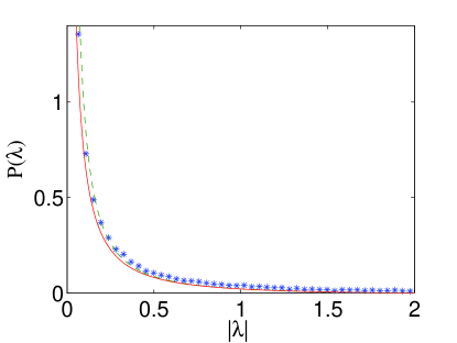
Figure 4: Distribution of the eigenvalues in two dimensions, for a low-density ($\frac{\xi}{r_{nn}}=0.05$). $N=1000$, and the results were obtained after averaging over 1000 instances. The points were distributed uniformly in the unit square, and the matrix element $A_{ij}=e^{-\frac{d_{ij}}{\xi}}$, with $\xi=0.0016$. The dashed curve is a plot of Eq. (15), while the solid curve is a plot of Eq. (21).

III.3 Relaxation of the conductance

In many cases a logarithmic relaxation in time is observed for the conductance Martinez ; Zvi:5 ; grenet2 . One should ask what is the relation between the relaxation of the conductivity and that of the occupations, for the electron glass model.

We now present an intuitive argument motivating the speculation that the time-relaxation of the conductance should be similar to that of the occupations. The essence of the argument is the claim that any perturbation of the equilibrium configuration will lead to enhanced conductance: if this is true, it is reasonable that as the typical deviation of the occupation number relaxes, so does the enhanced conductivity, until it reaches its equilibrium value. For small enough deviations, the two will be proportional to each other, as one can always take the lowest order term in the expansion of the dependence of the out-of-equilibrium conductivity on the occupation number deviation.

Let us explain our claim that any perturbation will lead to enhanced conductivity. This may come about by two physically different mechanism: first of all, we note that when the system is excited, we create vacant sites well below the Fermi surface, and add electrons above it. Electrons will tunnel between these sites, and thus even at very low temperatures current may flow through the system.

The second mechanism is more subtle, and is related to the Coulomb gap. Let us look at the Einstein relation imry_mesoscopics , $\sigma=e^{2}\frac{dn}{d\mu}D$. We do not expect to have any anomalies in the thermodynamic DOS, $\frac{dn}{d\mu}$, but the diffusion constant $D$ should be much smaller. This is because the single-particle DOS at the chemical potential vanishes: moving an electron from a site with energy close to the chemical potential to another site, will necessitate an energy of order of the width of the Coulomb gap. Therefore the Coulomb gap significantly lowers the conductivity. We shall assume that for a finite, large enough, single-particle DOS at $\mu$, the conductivity increases with the single-particle DOS at $\mu$ yu (for systems close to a local equilibrium, which exhibit the Coulomb gap). The temperature should be low enough such that the local equilibrium Coulomb gap would not be smeared T_c . Let us suppose that due to our initial perturbation of the local equilibrium configuration, we have some excess (positive or negative) $\delta n_{i}$ in the occupation number at site $i$. Assuming these numbers to be random with a standard deviation $\delta n$, the energy at site $j$ will now have an additional contribution $\sum_{i}{\frac{\delta n_{i}}{r_{ij}}}$. A finite single-particle DOS at $\mu$ will arise, proportional to $\delta n$. Both mechanisms show that within this model the conductance relaxation should have a similar time-dependence to that of the occupation number relaxation.

IV Conclusions

We have studied a finite temperature mean-field model for the dynamics of the electron glass system. For a perturbation which drives the system not too far from the (mean-field) local equilibrium, we mapped the problem onto rate equations with a random relaxation matrix $A$. The matrix $A$ belongs to a class different than the gaussian random matrix ensembles. We found that the distribution of the eigenvalues is approximately $\sim\frac{1}{|\lambda|}$, and naturally yields a logarithmic decay of the occupation numbers. This may lead to a logarithmic decay of the conductance. Such a logarithmic decay of the conductance is observed experimentally in many cases. We emphasize the remark made before that the $\frac{1}{\lambda}$ distribution of decay eigenvalues should be much more general than for the specific model considered. It might also hold, for example, in the case of multi-particle transitions, which are believed to be relevant for the long time properties of glasses. Further research is needed to obtain additional predictions of this model, such as the time-dependence of the Coulomb gap, and the voltage-dependent conductance in the ’two-dip’ experiment Zvi:4 .

References

- (1) D. Monroe et al., Phys. Rev. Lett. 59, 1148 (1987).
- (2) Z. Ovadyahu, Phys. Rev. B 48, 15025 (1993).
- (3) G. Martinez-Arizala et al., Phys. Rev. B 57, R670 (1998).
- (4) Z. Ovadyahu, Phys. Rev. Lett. 92, 066801 (2004).
- (5) J. Jaroszynski and D. Popovic, Phys. Rev. Lett. 96, 214208 (2006).
- (6) For two-dimensions and weak disorder, the density should be larger than , see T_c .
- (7) Z. Ovadyahu, Phys. Rev. Lett. 81, 669 (1998).
- (8) Z. Ovadyahu, Phys. Rev. B 65, 134208 (2002).
- (9) Z. Ovadyahu, Phys. Rev. Lett. 84, 3402 (2000).
- (10) T. Grenet, Eur. Phys. J. B 32, 275 (2003).
- (11) T. Grenet, Phys. Stat. Sol. (c) 1, 9 (2004).
- (12) B. Shklovskii and A. Efros, Electronic properties of doped semiconductors (Springer-Verlag, Berlin, 1984).
- (13) A. Miller and E. Abrahams, Phys. Rev. 120, 745 (1960).
- (14) A. J. Leggett et al., Rev. Mod. Phys. 59, 1 (1987).
- (15) M. Mezard, G. Parisi, and M. A. Virasoro, Spin glass theory and beyond (World Scientific, Singapore, 1987).
- (16) See, for example, spin_glass , p. 15.
- (17) M. Grunewald, B. Pohlmann, L. Schweitzer, and D. Wurtz, J. Phys. C: Solid State Phys., 15, L1153 (1982).
- (18) The critical temperature in dimension can be shown to be of order .
- (19) A. L. Efros, J. Phys. C: Solid State Phys 9, 2021 (1976).
- (20) T. Vojta, W. John, and M. Schreiber, J . Phys.: Condens. Matter 5, 4989 (1993).
- (21) M. Muller and S. Pankov, Phys. Rev. B. 75, 144201 (2007).
- (22) V. Malik and D. Kumar, Phys. Rev. B. 76, 125207 (2007).
- (23) J. G. Massey and M. Lee, Phys. Rev. Lett. 75, 4266 4269 (1995).
- (24) W. Mason, S. Kravchenko, G. Bowker, and J. Furneaux, Phys. Rev. B. 52, 7857 (1995).
- (25) N. F. Mott, Phil. Mag. 19, 835 (1969).
- (26) A. Y. Rogatchev and U. Mizutani, Phys. Rev. B. 61, 15550 (2000).
- (27) M. Mehta, Random Matrices (Academic Press, New York, 1991).
- (28) M. Mezard, G. Parisi, and A. Zee, Nuclear Physics B 3, 689 (1999).
- (29) P. Dutta and P. M. Horn, Rev. Mod. Phys. 53, 497 (1981).
- (30) Z. Ovadyahu and M. Pollak, Phys. Rev. B 68, 184204 (2003).
- (31) Y. Imry, Introduction to mesoscopic physics (Oxford University Press, New York, 1997).
- (32) C. C. Yu, Phys. Rev. Lett. 82, 4074 (1999).