ABILITIES OF MULTIDIMENSIONAL GRAVITY

K.A. Bronnikov† and S.G. Rubin‡

†

Centre for Gravitation and Fundamental Metrology, VNIIMS, 46 Ozyornaya St., Moscow, Russia;
Institute of Gravitation and Cosmology, PFUR, 6 Miklukho-Maklaya St., Moscow 117198, Russia

‡

Moscow Engineering Physics Institute, 31 Kashirskoe Shosse, Moscow 115409, Russia

We show that a number of problems of modern cosmology may be addressed and solved in the framework of multidimensional gravity with high-order curvature invariants, without invoking other fields. As applications of this approach, we mention primordial inflation and particle production after it; description of the modern accelerated stage of the Universe with stable compact extra dimensions; construction of asymmetric thick brane-world models.

1. Introduction

We consider multidimensional gravity as a basis for solving many fundamental problems using a minimal set of postulates. The particular value of the total space-time dimension $D>4$ and the topological properties of space-time are supposed to be determined by quantum fluctuations and may vary from one space-time region to another, leading to drastically different universes. It turns out that different effective theories take place even with fixed parameters of the original Lagrangian.

As a result, the situation to a certain extent resembles the prediction of string theory known as the landscape concept: the total number of different vacua in heterotic string theory is about $10^{1500}$ [1, 2]). The number of possible different universes is then huge but finite. Moreover, the concept of a random potential [3], also referring to quantum fluctuations, leads to an infinite number of universes with various properties. We make a step further and try to ascribe the origin of such potentials to multidimensional curvature-nonlinear gravity. We then use the obtained effective theories, containing scalar fields of purely geometric origin, to a number of well-known problems of modern cosmology.

Some challenging problems are those related to fine tuning, required to explain the actual properties of our Universe. Thus, small parameters are necessary to provide the smallness of temperature fluctuations of the CMB; an extremely small parameter is required to explain the observed value of dark energy density. It can be shown, in particular, that such fine-tuning problems may be reduced to the problem of the number of extra dimensions [4].

2. $F(R)$ gravity, a single factor space

2.1. Basic equations

Let us first consider, for simplicity, $D$-dimensional space-time with the structure ${\mathbb{M}}_{D}={\mathbb{M}}_{d}\times{\mathbb{M}}_{4}$, where the extra factor space ${\mathbb{M}}_{d}$ is of arbitrary dimension $d$ and is assumed to be a space of positive or negative constant curvature $k=\pm 1$. Consider the action

$$S={{\displaystyle\frac{1}{2}}}m_{\scriptscriptstyle D}^{D-2}\int\sqrt{{}^{D}g}\,d^{D}x\,[F(R)+L_{m}]$$ (1)

and the $D$-dimensional metric

$$ds^{2}=g_{\mu\nu}(x)dx^{\mu}dx^{\nu}+{\,\rm e}^{2\beta(x)}h_{ab}dx^{a}dx^{b}$$ (2)

where $(x)$ means the dependence on $x^{\mu}$, the coordinates of ${\mathbb{M}}_{4}$; $h_{ab}$ is the $x$-independent metric in ${\mathbb{M}}_{d}$. The choice (2) is used in many studies, e.g., [5, 6, 7].

Capital Latin indices cover all $D$ coordinates, small Greek ones cover the coordinates of ${\mathbb{M}}_{4}$ and $a,b,\ldots$ the coordinates of ${\mathbb{M}}_{d}$. The $D$-dimensional Planck mass $m_{\scriptscriptstyle D}$ does not necessarily coincide with the conventional Planck scale $m_{4}$; $m_{\scriptscriptstyle D}$ is, to a certain extent, an arbitrary parameter, but on observational grounds it must not be smaller than a few TeV.

The Ricci scalar can be written in the form

$$R = R_{4}+\phi+f_{\rm der},$$

$${}\phi = kd(d-1)m_{\scriptscriptstyle D}^{2}{\,\rm e}^{-2\beta(x)}$$

$${}f_{\rm der} = 2dg^{\mu\nu}\nabla_{\mu}\nabla_{\nu}\beta+d(d+1)(\partial\beta)^{2},$$ (3)

where $(\partial\beta)^{2}=g^{\mu\nu}\partial_{\mu}\beta\partial_{\mu}\beta$. The slow-change approximation, suggested in [4], assumes that all quantities are slowly varying, i.e., it considers each derivative $\partial_{\mu}$ (including those in the definition of $R_{4}$) as an expression containing a small parameter $\varepsilon$, so that

$$|\phi|\gg|R_{4}|,\ |f_{\rm der}|.$$ (4)

As shown in [4], this approximation even holds in any inflationary model whose characteristic energy scale is far below the Planck scale $m_{\scriptscriptstyle D}$, to say nothing of the modern epoch. Thus, the GUT scale, which is common in inflationary models, is $m_{\rm GUT}\sim 10^{-3}m_{4}$, which means that primordial inflation may be well described in the present framework if $m_{\scriptscriptstyle D}\sim m_{4}$.

In this approximation, using a Taylor decomposition for $F(R)=F(\phi+R_{4}+f_{\rm der})$, integrating out the extra dimensions and using a conformal mapping to pass over to a 4-dimensional Einstein frame with the metric ${\widetilde{g}}_{\mu\nu}$, we obtain up to $O(\varepsilon^{2})$:

$$S = \frac{{\cal V}[d]}{2}m_{\scriptscriptstyle D}^{2}\int d^{4}x\,\sqrt{{\widetilde{g}}}\,(\mathop{\rm sign}\nolimits F^{\prime})L,$$

$${}L = {\widetilde{R}}_{4}+{{\displaystyle\frac{1}{2}}}K_{\rm Ein}(\phi)(\partial\phi)^{2}-V_{\rm Ein}(\phi)+{\widetilde{L}}_{m},$$ (5)

$${}\hskip 28.45274pt{\widetilde{L}}_{m}=(\mathop{\rm sign}\nolimits F^{\prime})\frac{{\,\rm e}^{-d\beta}}{F^{\prime}(\phi)^{2}}L_{m};$$

$$K_{\rm Ein}(\phi) = \frac{1}{2\phi^{2}}\biggl{[}6\phi^{2}\biggl{(}\frac{F^{\prime\prime}}{F^{\prime}}\biggr{)}^{2}\!-2d\phi\frac{F^{\prime\prime}}{F^{\prime}}+{{\displaystyle\frac{1}{2}}}d(d+2)\biggr{]}\,,$$

$$V_{\rm Ein}(\phi) = -(\mathop{\rm sign}\nolimits F^{\prime})\left[\frac{|\phi|m_{\scriptscriptstyle D}^{-2}}{d(d-1)}\right]^{d/2}\frac{F(\phi)}{F^{\prime}(\phi)^{2}}.$$ (7)

In (5)–(7), the tilde marks quantities obtained from or with ${\widetilde{g}}_{\mu\nu}$; the indices are raised and lowered with ${\widetilde{g}}_{\mu\nu}$; everywhere $F=F(\phi)$ and $F^{\prime}=dF/d\phi$. All quantities of orders higher than $O(\varepsilon^{2})$ are neglected.

The quantity $\phi$ may be interpreted as a scalar field with the dimensionality $m_{\scriptscriptstyle D}^{2}$, see (2.1.). In what follows (if not indicated otherwise) we put $m_{\scriptscriptstyle D}=1$.

In fact, the function $F(\phi)$ represents an infinite power series inevitably caused by quantum corrections. Here we will use the truncated form

$$F(R)=R+cR^{2}+w_{1}R^{3}+w_{2}R^{4}-2\Lambda$$ (8)

and demonstrate that some new nontrivial results may be obtained even under such simplified assumptions. Curvature-quartic multidimensional models were also studied in [8].

2.2. Some applications

For certainty, we will everywhere treat the Einstein conformal frame, in which the Lagrangian has the form (5), as the physical frame used to interpret the observations. This assumption is not inevitable and is even rather arbitrary; the choice of a conformal frame is known to be related to the properties of the set of measurement instruments used [9, 10], and using other conformal frames is also possible but goes beyond the scope of this paper.

Effective particle production after inflation

According to [11], quick oscillations of the inflaton field immediately after the end of the inflationary stage are necessary for particle production which should lead to the observable amount of matter. It is known [12, 13] that if the inflaton coupling to matter fields is negligible, the mechanism of particle/entropy production and heating of the Universe could be ineffective. On the other hand, a strong coupling between the inflaton and matter fields, leading to large quantum corrections to the initial Lagrangian, would set to doubt the sufficiently small values of the input parameters needed for the very existence of the inflationary stage.

Another possibility of effective particle creation (parametric resonance) was described in [12]. Nonlinear multidimensional gravity yields one more mechanism [14].

Consider the potential and kinetic terms for the effective Lagrangian (5) with the function $F(R)$ taken from (8). A complicated $\phi$ dependence of the kinetic term strongly affects the classical scalar field dynamics. The effect is especially strong when the minimum of the kinetic term approximately coincides with that of the potential. To illustrate the situation, consider a toy model of a scalar field $\phi$ with

$$V(\phi) = \frac{1}{2}m^{2}\phi^{2}$$

$${}K(\phi) = K_{1}(\phi-\phi_{\min})^{2}+K_{\min},\quad K_{1},\ K_{\min}>0.$$ (9)

The field equations then read:

$${}H^{2}=\frac{\varkappa^{2}}{3}\left[\frac{1}{2}K(\phi)\dot{\phi}^{2}+V(\phi)\right],$$

$${}K(\phi)\left(\ddot{\phi}+3H\dot{\phi}\right)+\frac{1}{2}K_{\phi}(\phi)\dot{\phi}^{2}+V_{\phi}(\phi)=0$$ (10)

(the index $\phi$ means $d/d\phi$, and $H$ is the Hubble parameter).

When the inflation is over, the amplitude of inflaton oscillations is small at the Planck scale, and the effective kinetic term $K_{\rm eff}\sim K_{\min}$ is small due to the chosen values of the parameters. The effective Lagrangian, containing an interaction term of the inflaton and some other scalar field $\chi$

$$L_{\rm eff}\simeq\frac{1}{2}K_{\min}\dot{\phi}^{2}+g\phi\chi\chi,$$ (11)

can be brought into the standard form by re-definition of the inflaton field:

$$L_{\rm eff}\simeq\frac{1}{2}\dot{\phi}^{2}+\frac{g}{\sqrt{K_{\min}}}\phi\chi\chi.$$ (12)

A small value of $K_{\min}$ increases the effective coupling constant (by an order of magnitude for the chosen values of the parameters) and surely leads to more rapid particle production. As a result, we overcome the above difficulty: a slow motion during inflation may be reconciled with effective particle production right after inflation. Hence universes of this sort possess promising conditions for creation of complex structures.

Effect of the number and geometry of extra dimensions

Even if the initial Lagrangian is entirely specified, low-energy effective Lagrangians, drastically different from one another, can be obtained by varying $d$ and the curvature index $k$ of the extra dimensions.

A strong influence of the number $d$ on the effective Lagrangian parameters is evident since the potential (7) contains a quickly decreasing factor $\sim d^{-d}$. Thus, if in a stationary state $\phi=\phi_{0}$, the dimensionless initial parameters $|\phi_{0}|m_{\scriptscriptstyle D}^{-2}$ and $F^{\prime}(\phi_{0})$ are of order unity, the effective cosmological constant $\Lambda_{\rm eff}=V_{\rm Ein}(\phi_{0})$ is related to $F(\phi_{0})$ (which may be close to $m_{\scriptscriptstyle D}^{2}$) by

$$\Lambda_{\rm eff}/F(\phi_{0})\sim[d(d-1)]^{-d/2}.$$ (13)

It is of interest that $d^{-d}\approx 10^{-123}$ for $d=67$. Thus, at least in the Einstein picture, a fluctuation leading to a (67+4)-dimensional space may evolve to a space with the vacuum energy density $10^{-123}\,m_{4}$. The extreme smallness of $\Lambda_{\rm eff}$ is related to the number of extra dimensions, and other physical ideas are not required. We have taken for certainty $m_{\scriptscriptstyle D}=m_{4}$, otherwise the estimates will be slightly different.

Fig. 1 gives another example of $d$-dependence of the shape of the potential. Even its minimum does or does not exist depending on the value of $d$, see the curves at $\phi>0$. If a universe is nucleated with extra dimensions having negative curvature, we have $\phi<0$, see Fig. 1. Evidently the mean value of the potential $V(\phi)$ in such a universe tends to infinity for $d=2$, to a constant value for $d=4$ and to zero for $d=6$. All this takes place if the initial field value is less than $-1$. Otherwise, if a universe is born with $-1<\phi<0$, it is captured in a local minimum, and the size of extra dimensions remains small.

 

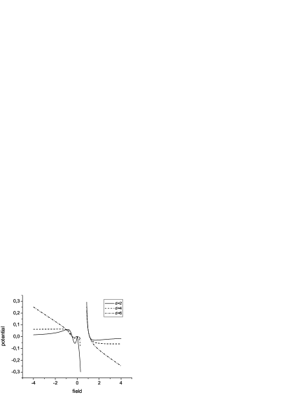
Figure 1: Different potentials for different $d$, obtained from the Lagrangian (5) with $F(R)$ in the form (8). Parameters: $c=0,\ w_{1}=0,\ w_{2}=-1,\ \Lambda=-0.25$. The curves are adapted to a unique scale.

3. Multiple factor spaces

So far we discussed effective low-energy theories corresponding to the metric (2) for different choices of the initial action. Some values of the parameters turned out to be suitable for the description of a universe like ours. Additional opportunities appear when varying the structure of extra dimensions, which includes the number of extra factor spaces, their dimensionality and curvature.

As was mentioned in the Introduction, we do not assume a specific number of extra dimensions or their topology. Both are thought to arise due to quantum fluctuations close to the Planck scale. If quantum fluctuations lead to a more complex structure of the extra dimensions, the physics becomes much richer.

3.1. Two compact extra factor spaces

Consider an extra space being a product of two factor spaces: ${\mathbb{M}}_{d}={\mathbb{M}}_{d_{1}}\times{\mathbb{M}}_{d_{2}}$, with the metric

$$ds^{2}=g_{\mu\nu}(x)dx^{\mu}dx^{\nu}+\sum_{i}{\,\rm e}^{2\beta_{i}(x)}h^{(i)}_{ab}dx^{a}dx^{b},$$ (14)

where the index $i=1,2$ enumerates the extra factor spaces and $h^{(i)}_{ab}$ have the same properties as $h_{ab}$ in the previous section, with the curvature indices $k_{i}=\pm 1$ similar to $k$ in (2.1.). Considering the same action (1), we should introduce two scalar fields

$$\phi_{i}=k_{i}(d_{i}-1)m_{\scriptscriptstyle D}^{2}{\,\rm e}^{-2\beta_{i}(x)}$$ (15)

to describe the low-energy limit. The effective potential has the following form in the Einstein frame:

$${}V_{\rm Ein}(\phi_{1},\phi_{2})$$

$${}=-\frac{1}{2}\frac{\big{(}\mathop{\rm sign}\nolimits F^{\prime}(\phi)\big{)}}{[F^{\prime}(\phi)]^{2}}\frac{|\phi_{1}|^{d_{1}/2}}{[(d_{1}{-}1)]^{d_{1}/2}}\frac{|\phi_{2}|^{d_{2}/2}}{[(d_{2}{-}1)]^{d_{2}/2}}$$

$${}\times\biggl{[}F(\phi)+d_{1}\phi_{1}^{2}\biggl{(}\!c_{1}+\frac{2c_{2}}{d_{1}{-}1}\!\biggr{)}+d_{2}\phi_{2}^{2}\biggl{(}\!c_{1}+\frac{2c_{2}}{d_{2}{-}1}\!\biggr{)}\biggr{]},$$

where $\phi=d_{1}\phi_{1}+d_{2}\phi_{2}$.

 

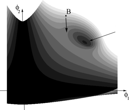
Figure 2: Effective potential for an extra space with the topology ${\mathbb{M}}_{d}={\mathbb{M}}_{d_{1}}\times{\mathbb{M}}_{d_{2}}$, $d_{1}=d_{2}=3$, and the parameters are $c=-0.5,\ \Lambda=0.2,\ c_{1}=c_{2}=-0.38$. The view is from above, lower levels are darker. The local minimum is marked by a long arrow.

It is presented in Fig. 2 where two valleys of the potential lie in perpendicular directions, $\phi_{1}=0$ and $\phi_{2}=0$, each of them corresponding to an infinite size of one of the extra factor spaces, ${\mathbb{M}}_{d_{1}}$ or ${\mathbb{M}}_{d_{2}}$. Of greater interest is the local minimum, marked by a long arrow, where both factor spaces are compact and have a finite size. A universe can live long enough in this metastable state, as in the case of a simpler topology of extra dimensions discussed above.

An interesting possibility arises if a universe is formed at point B in Fig. 2. There occurs inflation, and it ends as the fields move from point B along the arrow. The fate of different spatial domains depends on the field values in these domains. Even if most of them evolve to the metastable minimum, some part of the domains overcome the saddle and tend to the first or second valley, with an infinite size of one of the factor spaces. In this case, our Universe should contain some domains of space with macroscopically large extra dimension. Their number and size crucially depend on the initial conditions.

The laws of physics in such a domain are quite different from ours. So, if, say, a star enters into such a domain, since the law of gravity is dimension-dependent, the balance of forces inside the star will be violated, and it will collapse or decay. More than that, there will be no usual balance between nuclear and electromagnetic forces in the stellar matter, so that even nuclei (except maybe protons) will decay as well. Even hadrons, being composite particles, are likely to lose their stability.

3.2. Thick asymmetric brane world models

Quite a different configuration is obtained if, again using the metric (14), we assume that one of the extra factor spaces is noncompact, thus considering a mixed ansatz: let, say, ${\mathbb{M}}_{d_{1}}$ be noncompact and, for simplicity, one-dimensional ($d_{1}=1$) while ${\mathbb{M}}_{d_{2}}$ is, as before, a compact factor space in the spirit of the Kaluza-Klein concept. As a result of the reduction procedure described above, we obtain (in the Einstein frame) an effective 5D theory in the space-time ${\mathbb{M}}_{5}={\mathbb{M}}_{4}\times{\mathbb{M}}_{d_{1}=1}$ with the Lagrangian [15]

$$L_{\rm eff}=R_{5}+K(\phi)g^{ab}\partial_{a}\phi\partial_{b}\phi-2V(\phi),$$ (17)

where $R_{5}$ is the 5D Ricci scalar, $\phi$ is an effective scalar field, obtained in the above manner from the scale factor of ${\mathbb{M}}_{d_{2}}$, and we have chosen the units so that the effective 5D gravitational constant is equal to unity. The indices $a,b$ cover all five coordinates. The functions $K(\phi)$ and $V(\phi)$ are obtained from the initial $D$-dimensional action similarly to the quantities $K_{\rm Ein}$ and $V_{\rm Ein}$ in Eqs. (2.1.), (7). The 5D metric is chosen in the form

$$ds^{2}={\,\rm e}^{2\gamma(y)}dt^{2}-{\,\rm e}^{2\beta(y)}d{\vec{x}}{}^{2}-dy^{2},$$ (18)

where $\{\vec{x},t\}$ are the usual 4D coordinates and $y$ is the fifth coordinate. Assuming global regularity, we seek models of thick brane worlds able to trap ordinary matter in some layer described by a small range of the coordinate $y$.

Many models of interest can be obtained if we use a more general initial action than (1), namely,

$${}S={{\displaystyle\frac{1}{2}}}m_{\scriptscriptstyle D}^{D-2}\!\int\!\sqrt{{}^{D}g}\,d^{D}x\Big{[}F(R)$$

$${}\hskip 72.26999pt\hskip 28.45274pt+c_{1}R_{AB}R^{AB}+c_{2}{\cal K}\Big{]},$$ (19)

where $R_{AB}$ is the Ricci tensor and ${\cal K}=R_{ABCD}R^{ABCD}$ is the Kretschmann scalar in ${\mathbb{M}}_{D}$; $c_{1}$ and $c_{2}$ are constants, and we take, as before, the function $F(R)$ in the form (8). It should be noted that the reduction procedure, involving the slow-change approximation, works well with this more general action (and even more complex ones) and leads to effective 5D Lagrangians of the form (17).

 

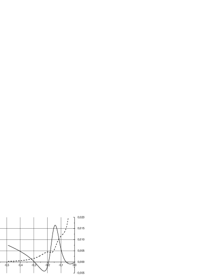
Figure 3: The parameter values given in Eq. (3.2.). The solid line shows the potential, the dashed line represents the kinetic term multiplied by the factor $10^{-5}$.

Fig. 2 presents an example of the functions $V(\phi)$ and $K(\phi)$ corresponding to the parameters

$${}d_{0}=5,\ \ d_{1}=2,\ \ c=6,\ \ w_{1}=15,\ \ w_{2}=7,$$

$${}\hskip 28.45274pt\Lambda=-0.02,\ \ c_{k}=4(c_{1}+c_{2})=5,$$

$${}\hskip 28.45274ptc_{v}=c_{1}+2c_{2}/(d_{2}-1)=1.5,$$ (20)

which give rise to an asymmetric thick brane in 5D space, similar in its main features to the second Randall–Sundrum model (RS2) [16]. The corresponding solution to the field equations that follow from (17) describes a space-time with the metric (18) which is asymptotically anti-de Sitter (AdS) at large $|y|$, with the decressing warp factor ${\,\rm e}^{\gamma}={\,\rm e}^{\beta}\sim{\,\rm e}^{-k_{\pm}|y|}$, though with different curvature values as $y\to+\infty$ and $y\to-\infty$ ($k_{+}\neq k_{-})$; the scalar field $\phi$ has the conventional form of a kink interpolating between two minima of the potential while $K(\phi)$ remains positive. Like the RS2 branes, these configurations have AdS horizons at both sides far from the brane; they are able to trap a massless scalar field and, since gravitational perturbations are known to behave as a massless scalar [17], such models naturally provide the validity of Newton’s law with proper corrections [16, 18] for matter on the brane. Assuming that the brane asymmetry is negligible, approximate expressions for the modified Newtonian potential $V_{N}$ for gravity on the brane at large and small radii $R$ are [19]

$${}V_{N}(R)\approx-\frac{GM}{R}\biggl{(}1+\frac{2l_{c}}{3R}\biggr{)},\hskip 28.45274pt\ R\ll l_{c},$$

$${}V_{N}(R)\approx-\frac{GM}{R}\biggl{(}1+\frac{2l_{c}}{3R^{2}}\biggr{)},\hskip 28.45274ptR\gg l_{c}.$$ (21)

where $l_{c}$ is the mean AdS curvature radius. At radii $\gtrsim 10\,l_{c}$, the potential almost coincides with the Newtonian one while at small radii as compared with $l_{c}$ (but large as compared with the brane width) gravity becomes effectively 5-dimensional. The Newtonian gravitational constant $G$ is related to the 5D Planck mass $m_{5}$ as follows:

$$8\pi G=(m_{5}^{3}l_{c})^{-1},$$ (22)

where $m_{5}$ is connected with the initial multidimensional Planck mass $m_{\scriptscriptstyle D}$ by a coefficient of order unity.

A well-known problem with such branes is their inability to trap massive scalar fields [20].

A peculiar feature of another class of BW models obtained from (17) (with other sets intial parameters) is that $K(phi)$ has a variable sign, i.e., the scalar kinetic energy is positive in some range of $\phi$ values and negative in another range. The brane is located in the vicinity of the transition point between these ranges and is thus highly asymmetric by construction. In such BW models, the warp factor again corresponds to AdS space far from the brane, but exponentially grows, which provides a purely gravitational mechanism for matter field trapping, without need for any interaction between $\phi$ and matter fields [20]. There is a problem with massless field and graviton trapping since it turns out that the discrete spectrum of trapped scalar field modes does not contain a massless mode. These branes are, however, similar to one of the two branes in the RS1 model [21], namely, the one with negative tension, which is interpreted as the observable (Planck) brane, and Newton’s law with certain corrections is known to hold there [21, 22, 23]. Our models can be interpreted in terms of an RS1-like structure, with a circular extra dimension, but with a positive-tension brane moved to infinity. In this case, a viable law of gravity on the brane can be obtained and may be written as [15]

$${}V_{N}(R)\approx-\frac{G_{1}l_{c}M}{3\pi R^{2}},\hskip 28.45274ptR\ll l_{c},$$

$${}V_{N}(R)\approx-\frac{G_{1}M}{3R},\hskip 28.45274pt\ R\gg l_{c}.$$ (23)

where $8\pi G_{1}=1/(m_{5}^{3}l_{c})$. Thus, for $R\gg l_{c}$, Newton’s law is valid with the gravitational constant $G=G_{1}/3$ (whereas in (3.2.) we had $G=G_{1}$); at small radii, as before, the potential is proportional to $R^{-2}$, though with another coefficient.

The AdS curvature radius $l_{c}$ remains an arbitrary parameter in all such models.

4. Conclusion

We have discussed the ability of nonlinear multidimensional gravity to produce various low-energy effects and models, some of which could describe our Universe. We only assume a certain form of the pure gravitational action and a sufficient number of extra dimensions but do not fix the number, dimensions and curvature signs of extra factor spaces. Artificial inclusion of matter fields is not supposed, so that our conclusions are based on purely geometric grounds.

We have seen that the same theory described by a specific Lagrangian leads to a diversity of low-energy situations, depending on the structure of extra dimensions and the initial conditions.

We have found out, in particular, that nontrivial forms of the kinetic term of the inflaton field arise naturally in this approach. As a result, inflaton oscillations at the end of inflation could be very rapid with an appropriate form of the kinetic term. This increases the particle production rate after the end of inflation. At the same time, a slow motion of the inflaton at the beginning of inflation provides a sufficiently long inflationary stage.

It has also been shown that multiple production of closed walls and hence massive primordial black holes is a probable consequence of modern models of inflation [24].

Quite different effective low-energy models arise if one considers different numbers and/or topology of extra dimensions, even if all parameters of the initial Lagrangian are fixed. It means that the specific values of these parameters could be less important than it is usually supposed: even more important are the number, dimensions and curvatures of the extra factor spaces. In particular, varying the number $d$ of extra dimensions forming a single factor space, it is quite easy to obtain the proper value of the inflaton mass.

We have seen that the size of extra dimensions may depend on the spatial point in the observed space, so that our Universe may contain spatial domains with a macroscopic size of extra dimensions, where the whole physics should become effectively multidimensional.

We have also obtained 5D gravitational kinky configurations which could be interpreted as thick branes in the spirit of the widely discussed brane world concept.

Thus pure multidimensional gravity, even without other ingredients, is quite a rich structure, and many problems of modern cosmology may be addressed in this framework. A task of interest is to try to construct a model able to solve a number of such problems (if not all) simultaneously.

Acknowledgement

K.B. acknowledges partial financial support from Russian Basic Research Foundation Projects 05-02-17478 and 07-02-13614-ofi-ts.

References

- [1] W. Lerche, D. Lust and A.N. Schellekens, “Chiral four-dimensional heterotic strings from selfdual lattices”, Nucl. Phys. B 287, 477 (1987).
- [2] S. Kachru, R. Kallosh, A. Linde and S. P. Trivedi, “De Sitter vacua in string theory”, Phys. Rev. D 68, 046005 (2003); hep-th/0301240.
-
[3]
S.G. Rubin, “Fine tuning of parameters of the Universe”.
Chaos Solitons Fractals 14, 891, 2002; astro-ph/0207013;
S.G. Rubin, “Origin of universes with different properties”, Grav. & Cosmol. 9, 243-248, 2003; hep-ph/0309184. - [4] K.A. Bronnikov and S.G. Rubin, “Self-stabilization of extra dimensions”, Phys. Rev. D 73, 124019 (2006); gr-qc/0510107.
- [5] U. Günther, P. Moniz and A. Zhuk, “Multidimensional cosmology and asymptotical ADS”, Astrophys. Space Sci. 283, 679-684 (2003); gr-qc/0209045.
- [6] R. Holman et.al, Phys. Rev. D 43, 1991.
- [7] A.S. Majumdar and S.K. Sethi, Phys. Rev. D 46, 5315 (1992).
- [8] U. Günther, A. Zhuk, V.B. Bezerra and C. Romero, Class. Quant. Grav. 22, 3135 (2005); hep-th/0409112. T. Saidov and A. Zhuk, Gravitation & Cosmology, 12, 253 (2006), hep-th/0604131.
- [9] K.P. Staniukovich and V.N. Melnikov, “Hydrodynamics, Fields and Constants in the Theory of Gravitation”, Energoatomizdat, Moscow, 1983 (in Russian).
- [10] K.A. Bronnikov and V.N. Melnikov, in: Proceedings of the 18th Course of the School on Cosmology and Gravitation: The Gravitational Constant. Generalized Gravitational Theories and Experiments, Erice, 2003, ed. by G.T. Gillies, V.N. Melnikov and V. de Sabbata (Kluwer, Dordrecht/Boston/London, 2004), p. 39.
-
[11]
A.D. Dolgov and A.D. Linde, Phys. Lett. 116B, 329 (1982);
L.F. Abbott, E. Fahri and M. Wise, Phys. Lett. 117B, 29 (1982). - [12] L. Kofman, A. Linde and A. Starobinsky, “Reheating after inflation”, Phys. Rev. Lett. 73, 3195-3198 (1994); hep-th/9405187.
- [13] Y. Shtanov, J. Traschen and R. Brandenberger, “Universe reheating after inflation”, hep-ph/9407247.
- [14] K.A. Bronnikov, R.V. Konoplich and S.G. Rubin, “The diversity of universes created by pure gravity”, Class. Quantum Grav. 24, 1261–1277 (2007).
- [15] K.A. Bronnikov and S.G. Rubin, “Thick branes from nonlinear multidimensional gravity”, Grav. & Cosmol. 13, 191 (2007).
- [16] L. Randall and R. Sundrum. Phys. Rev. Lett. 83, 3690 (1999).
- [17] O. DeWolfe, D.Z. Freedman, S.S. Gubser and A. Karch, “Modeling the fifth dimension with scalars and gravity”, Phys. Rev. D 62, 046008 (2000); hep-th/9909134.
- [18] N. Deruelle and M. Sasaki, Progr. Theor. Phys. 110, 441 (2003); gr-qc/0306032.
- [19] P. Callin and F. Ravndall, Phys. Rev. D 70, 104009 (2004); hep-ph/0403302.
-
[20]
K.A. Bronnikov and B.E. Meierovich,
“A general thick brane supported by a scalar field”.
Grav. & Cosmol. 9, 313 (2003); gr-qc/0402030;
S.T. Abdyrakhmanov, K.A. Bronnikov and B.E. Meierovich, “Uniqueness of RS2 type thick branes supported by a scalar field”. Grav. & Cosmol. 11, 75 (2005); gr-qc/0503055. - [21] L. Randall and R. Sundrum. Phys. Rev. Lett. 83, 3370 (1999).
- [22] M.N. Smolyakov and I.P. Volobuev, “Linearized gravity, Newtonian limit and light deflection in RS1 model”, hep-th/0208025.
- [23] R. Arnowitt and J. Dent, “Gravitational forces on the branes”. Phys. Rev. D 71, 124024 (2005); hep-th/0412016.
- [24] S.G. Rubin, “Massive primordial black holes in hybrid inflation”. In: “Moscow 2003, I. Ya. Pomeranchuk and physics at the turn of the century”, pp. 413–418; astro-ph/0511181.