Critical line in undirected Kauffman boolean networks - the role of percolation

Abstract

We show that to correctly describe the position of the critical line in the Kauffman random boolean networks one must take into account percolation phenomena underlying the process of damage spreading. For this reason, since the issue of percolation transition is much simpler in random undirected networks, than in the directed ones, we study the Kauffman model in undirected networks. We derive the mean field formula for the critical line in the giant components of these networks, and show that the critical line characterizing the whole network results from the fact that the ordered behavior of small clusters shields the chaotic behavior of the giant component. We also show a possible attitude towards the analytical description of the shielding effect. The theoretical derivations given in this paper quite tally with numerical simulations done for classical random graphs.

1 Introduction

Almost 40 years ago Stuart Kauffman proposed random Boolean networks (RBNs) for modelling gene regulatory networks [1]. Since then, beside its original purpose, the model and its modifications have been applied to many different phenomena like cell differentiation [2], immune response [3], evolution [4], opinion formation [5], neural networks [6], and even quantum gravity problems [7].

The original RBNs were represented by a set of $N$ elements, $\sum_{t}=\{\sigma_{1}(t),\sigma_{2}(t),...,\sigma_{N}(t)\}$, each element $\sigma_{i}$ having two possible states: active ($1$), or inactive ($0$). The value of $\sigma_{i}$ was controlled by $k$ other elements of the network, i.e.

$$\sigma_{i}(t+1)=f_{i}(\sigma_{i_{1}}(t),\sigma_{i_{2}}(t),...,\sigma_{i_{k}}(t)),$$ (1)

where $k$ was a fixed parameter. The functions $f_{i}$ were selected so that they have returned values $1$ and $0$ with probabilities respectively equal to $p$ and $1-p$. The parameters $k$ and $p$ have determined the dynamics of the system (Kauffman network), and it has been shown that for a given probability $p$, there exists the critical number of inputs [13]

$$k_{c}=\frac{1}{2p(1-p)},$$ (2)

below which all perturbations in the initial state of the system die out (frozen phase), and above which a small perturbation in the initial state of the system may propagate across the entire network (chaotic phase).

In fact, the behavior of Kauffman model in the vicinity of the critical line $k_{c}(p)$ has become a major concern of scientists interested in gene regulatory networks. The main reason for this was the conjecture that living organisms operate in a region between order and complete randomness or chaos (the so-called edge of chaos) where both complexity and rate of evolution are maximized [8, 9, 10]. The analogous behavior has been noticed in Kauffman networks, which in the interesting region described by eq. (2) show stability, homeostatis, and the ability to cope with minor modifications when mutated. The networks are stable as well as flexible in this region.

Recently, when data from real networks have become available [11, 12], a quantitative comparison of the edge of chaos in these datasets and RBN models has brought an encouraging and promising message that even such simple model may quite well mimic characteristics of real systems.

Since, however, one has noticed that real genetic networks exhibit a wide range of connectivities, the recent modifications of the standard RBN take into consideration a distribution of nodes’ degrees $P(k)$. It has been shown that if the random topology of the directed network is homogeneous (i.e. all elements of the network are statistically equivalent), then the network topology can be meaningfully characterized by the average in-degree $\langle k\rangle$, and the transition between frozen and chaotic phase occurs for [14]:

$$\langle k\rangle_{c}=\frac{1}{2p(1-p)}.$$ (3)

Several authors [17, 18] have provided a general formula for the edge of chaos in directed networks characterized by the joint degree distribution $P(k,q)$

$$\frac{\langle kq\rangle}{\langle q\rangle}=\frac{1}{2p(1-p)},$$ (4)

where $k$ and $q$ correspond to in- and out-degrees of the same node, respectively. The formula (4) shows that the position of the critical line depends on the correlations between $k$ and $q$ in such networks. It is also easy to show that the previous results (2) and (3) immediately follow from (4) if one assumes the lack of correlations $P(k,q)=P_{in}(k)P_{out}(q)$.

Very recently, it has been shown by finite size scaling methods (FSS) that the critical connectivity $\langle k\rangle_{c}^{FSS}$ significantly deviates from the value established by the Eq. (3), even for large system sizes [19]. More precisely, one observes that $\langle k\rangle_{c}^{FSS}<\langle k\rangle_{c}$. To support the observation the authors recall other studies [20] which suggest that gene regulatory networks appear to be in the ordered regime and reside slightly below the phase transition between order and chaos in opposite to the theory which proposes the critical line to be an evolutionary attractor.

In the present paper, we suggest other explanation of the observed discrepancy. We show (both analytically and numerically) that the discrepancies are due to the percolation phenomena, which become important in the region of small values of the parameter $\langle k\rangle$.

To understand the complexity of percolation phenomena in directed graphs let us recall the structure of such a graph [23, 26]. In general, a directed graph consists of a giant weakly connected component (GWCC) and several finite components (FCs). In the GWCC every site is reachable from every other, provided that the links are treated as bidirectional. The GWCC is further divided into a giant strongly connected component (GSCC), consisting of all sites reachable from each other following directed links. All sites reachable from the GSCC are referred to as the giant OUT component, and the sites from which the GSCC is reachable are referred to as the giant IN component. The GSCC is the intersection of the IN and OUT components. All sites in the GWCC, but not in the IN and OUT components, are referred to as the tendrils (TDs) (see Fig. 1).

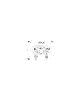
Figure 1: General structure of a directed network above the percolation threshold.

Size of all components listed above has doubtless impact on propagation of perturbations in directed RBNs. Moreover, GSCC and GWCC start to form at different values of the parameter $\langle k\rangle$ (see Fig. 2a). Although it has been shown [23, 26] how to find the relative sizes of the components (for example GWCC appears when $\langle kq\rangle\geq\langle q\rangle$), the problem of how to implement the results to the theory of perturbation spreading in RBNs is still far from being solved. To make the first step in this direction, and to show the importance of percolation phenomena on dynamics of RBN we concentrate on undirected case of the model. Although the original RBNs have been defined as directed ones, the study of undirected networks significantly reduces complexity of the problem (see Fig. 2).

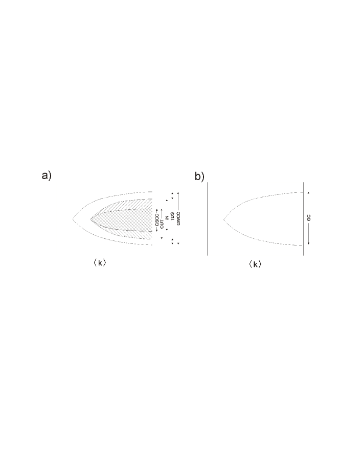
Figure 2: Schematic plot of sizes of network components as a function of average node degree in a) directed ER graphs and b) undirected ER graphs.

To this end, we organize the paper as follows. In the next section, we present numerical methodology and finite-size scaling of perturbation spreading in RBNs. In section 3 we derive general relation describing position of the critical line in undirected RBNs with arbitrary distribution of connections $P(k)$, in the analogy of the mean-field theory for directed RBNs [13]. Comparing the theory with numerical simulations we show significant deviations between the both approaches. Then an improved treatment including percolation phenomena is presented in section 4. A summary of our findings is given in section 5.

2 Critical line in undirected random graphs - numerical simulations

In order to find the position of the critical line in RBN one has to examine the sensitivity of its dynamics with regard to initial conditions. In numerical studies such a sensitivity can be analyzed quite simply. One has to start with two initial states $\sum_{0}=\{\sigma_{1}(0),\sigma_{2}(0),...,\sigma_{N}(0)\}$ and $\widetilde{\sum}_{0}=\{\widetilde{\sigma}_{1}(0),\widetilde{\sigma}_{2}(0),...,\widetilde{\sigma}_{N}(0)\}$, which are identical except for a small number of elements, and observe how the differences between both configurations $\sum_{t}$ and $\widetilde{\sum}_{t}$ change in time. If a system is robust then the studied configurations lead to similar long-time behavior, otherwise the differences develop in time. A suitable measure for the distance between the configurations is the overlap $x(t)$ defined as

$$x(t)=1-\frac{1}{N}\sum_{i=1}^{N}|\sigma_{i}(t)-\widetilde{\sigma}_{i}(t)|.$$ (5)

Note, that in the limit $N\rightarrow\infty$, the overlap becomes the probability for two arbitrary but corresponding elements, $\sigma_{i}(t)$ and $\widetilde{\sigma_{i}}(t)$, to be equal. Moreover, the stationary long-time limit of the overlap $x=\lim_{t\rightarrow\infty}x(t)$ can be treated as the order parameter of the system. If $x=1$ then the system is insensitive to initial perturbations (frozen phase), while for $x<1$, the initial perturbations propagate across the entire network (chaotic phase).

For numerical purposes we define the probability $D$ that the system is sensitive to perturbations

$$D=\frac{\sum_{x(t=T)<x(0)}^{R}1}{R},$$ (6)

where $R$ is the number of generated networks, and $T$ is the number of system updates. In our simulations we take $RN=10^{6}$ and $T=200$. The Fig. 3a presents a typical example of $D$ dependence on our control parameter $\langle k\rangle$ for different network sizes. Then, we apply finite-size scaling method [24] to determine how the probability $D$ scales with the system size. Around some critical point, we predict that systems of all sizes are indistinguishable except for a change of scale. This suggests

$$D(\langle k\rangle)=f(\phi),$$ (7)

where

$$\phi=\left(\frac{\langle k\rangle-\langle k\rangle_{c}}{\langle k\rangle_{c}}\right)N^{1/\nu}.$$ (8)

In Eq. (7), $f$ is one of the functions shown in the figure 3a, $\langle k\rangle_{c}$ is the critical point, and $N^{1/\nu}$ provides the change of scale. Fig. 3b shows how the probability $D$ depends on the parameter $\phi$ with fitted parameters $\langle k\rangle_{c}=1.45\pm 0.04$ and $\nu=2.2\pm 0.1$.

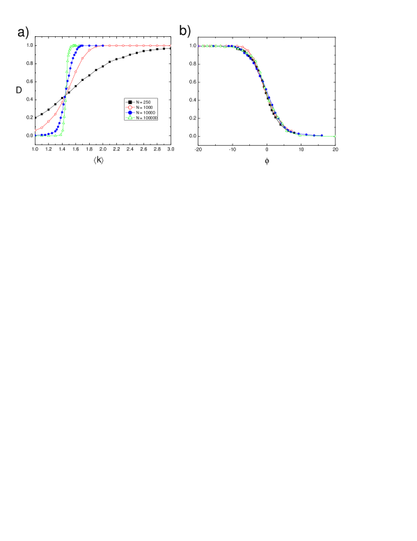
Figure 3: Probability $D$ against a) control parameter $\langle k\rangle$ and b) rescaled parameter $\phi$ for $p=0.5$.

The other problem which should be noted here is the observation that $\langle k\rangle_{c}$ depends on the number of initially perturbed nodes. In the Fig. 4 we plot the dependence of normalized critical connectivity

$$\widetilde{\langle k\rangle}_{c}=\frac{\langle k\rangle_{c}(\Delta)-\langle k\rangle_{c}}{\langle k\rangle_{c}},$$ (9)

against the number $\Delta$ of initially perturbed nodes in the network of $N=1000$ elements. For further calculations we choose $\Delta=0.032\;N$, since then the error in $\langle k\rangle_{c}$ is less than the error arising in finite-size scaling.

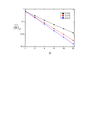
Figure 4: Normalized critical connectivity against the number of perturbed nodes in networks of $N=1000$ elements. Lines are shown only for better visibility of the presented dependence.

In Fig. 5, using the method described above, we show the numerically obtained values of $\langle k\rangle_{c}$ against the parameter $p$. For $p=0.5$ critical connectivity is minimal, i.e. $\langle k\rangle_{c}=1.45$. Please note that the size of the giant component for this connectivity is about one half of the whole network. One can expect that a large number of isolated nodes and clusters can significantly affect the perturbation spreading rate in this regime. Moreover, it has been demonstrated [25], that the giant component is correlated in sparse networks. In the following, we will show that a mean field theory which does not take into account these percolation and correlation issues, although correct for large values of $\langle k\rangle$, deviates from numerical results for $\langle k\rangle$ close to $1$.

Figure 5: Phase diagram for undirected RBN model. Points show results obtained by numerical simulations. The line is a solution of eq. (19).

3 Damage spreading in undirected Kauffman RBN - a simple approach

In this section, we derive a mean field formula for the critical line characterizing Kauffman boolean model in undirected and uncorrelated random graphs with arbitrary degree distributions $P(k)$. To this end, we partially reproduce and generalize a simple annealed calculations that have been for the first time carried out by Derrida and Pomeau [13]. The case of random directed networks has been studied by Aldana [15], and also by Lee and Rieger [17].

Thus, let $x_{i}(k,t)$ corresponds to the probability that a given element $i$ of degree $k$ possesses the same value in both configurations $\sum_{t}$ and $\widetilde{\sum}_{t}$ of the considered boolean network, i.e. $\sigma_{i}(t)=\widetilde{\sigma}_{i}(t)$. It occurs either when all the $k$ inputs of $\sigma_{i}(t)$ are equal to respective inputs of $\widetilde{\sigma}_{i}(t)$, or when the function $f_{i}$, cf. (1), ascribed to the node $i$ returns the same value for these two configurations. The first case happens with probability

$$X(q_{1},q_{2},\dots,q_{k},t-1)=x(q_{1},t-1)x(q_{2},t-1)\dots x(q_{k},t-1),$$ (10)

where $x(q_{j},t-1)$ represents probability that in the previous time step $(t-1)$ the $j$th nearest neighbor of $i$ having degree $q_{j}$ was in the same state in the two considered configurations. It is also easy to see that the second case arises with probability $p^{2}+(1-p)^{2}$, when at least one of the $k$ inputs of $\sigma_{i}$ differs from its counterpart in $\widetilde{\sigma}_{i}$ giving rise to the same values of $\sigma_{i}$ and $\widetilde{\sigma}_{i}$. Such a situation, in turn, happens with probability equal to $1-X(q_{1},q_{2},\dots,q_{k},t-1)$. Taking all the above together we find that the probability $x_{i}(k,t)$ that $\sigma_{i}(t)=\widetilde{\sigma}_{i}(t)$ is given by

$$x_{i}(k,t+1) = X(q_{1},\dots,t)+(p^{2}+(1-p)^{2})X(q_{1},\dots,t)$$ (11)

$$= 1-2p(1-p)\left(1-X(q_{1},q_{2},\dots,q_{k},t)\right),$$

where $q_{1},q_{2},\dots,q_{k}$ stand for degrees of nodes found in the nearest neighborhood of the node $i$.

The equation (11) describes dynamics of a single node $i$ of degree $k$. In order to study boolean dynamics of the whole network one has to average the equation, first over the nearest neighborhood of $i$, next over the whole network. The first step simply means averaging over the distribution $P(q_{1},q_{2},\dots,q_{k}/k)$, which describes probability that nearest neighbors of $i$ have degrees respectively equal to $q_{1},q_{2},\dots,q_{k}$

$$x(k,t+1)=1-2p(1-p)\left(1-\sum_{q_{1},\dots,q_{k}}X(q_{1},\dots,t)P(q_{1},\dots/k)\right),$$ (12)

whereas the second step corresponds to averaging of the last equation over the node degree distribution $P(k)$ characterizing the whole network. Note, that we have omitted the subscript $i$ at $x(k,t+1)$ in Eq. (12). After averaging, $x(k,t+1)$ refers to the set of nodes having the same degree $k$.

At the moment, before we proceed with our calculations let us outline structural properties of the studied networks. At the beginning let us remind that the assumed lack of higher-order correlations (e.g. three-point or four-point correlations) means that a given link $\{i,j\}$ does not influence other links of the considered nodes $i$ and $j$. It translates to the fact that the conditional probability $P(q_{1},q_{2},\dots,q_{k}/k)$ factorizes

$$P(q_{1},q_{2},\dots,q_{k}/k)=P(q_{1}/k)P(q_{2}/k)\dots P(q_{k}/k),$$ (13)

where $P(q_{j}/k)$ describes probability that a node of degree $q_{j}$ is the nearest neighbor of a node having degree $k$. Given the formulas (10), (13) and (15), the equation (12) further simplifies as follows

$$x(k)=1-2p(1-p)\left(1-\left(\sum_{q}x(q)P(q/k)\right)^{k}\right),$$ (14)

where, since we are interested in the stationary (i.e. for $t\rightarrow\infty$) solutions of this equation, we have omitted dependence on time $t$.

Figure 6: The map $y=M(y)$ considered in the text. The solid line corresponds to the situation when the only stable solution is $\langle kx\rangle=\langle k\rangle$, i.e. $x(k)=1$ for all values of $k$. The dashed line shows the case when the second solution $\langle kx\rangle<\langle k\rangle$ appears.

Now, assuming the lack of two point correlations, i.e.

$$P(q_{j}/k)=\frac{q_{j}}{\langle k\rangle}P(q_{j}),$$ (15)

which causes that the nearest neighborhood of each node is the same (in statistical terms), and then multiplying both sides of Eq. (14) by $k$, and finally averaging the resulting equation over the node degree distribution $P(k)$, we get the desired mean-field equation which describes stationary states of the Kauffman model defined on undirected and uncorrelated random networks with arbitrary degree distributions

$$\frac{\langle kx\rangle}{\langle k\rangle}=M\left(\frac{\langle kx\rangle}{\langle k\rangle}\right)=1-2p(1-p)\left(1-\sum_{k}\left(\frac{\langle kx\rangle}{\langle k\rangle}\right)^{k}\frac{k}{\langle k\rangle}P(k)\right),$$ (16)

where $\langle kx\rangle=\sum_{k}kx(k)P(k)$.

At the moment, note that the state $\langle kx\rangle=\langle k\rangle$, which in fact corresponds to the set of conditions $x(k)=1$ for all nodes’ degrees $k$, is always a solution of the last equation, see Fig. 6. Note also, that this solution may be stable or unstable depending on properties of the considered map $y=M(y)$, where $y=\langle kx\rangle/\langle k\rangle$ (16). In fact, one can show that the solution loses its stability, when another solution $\langle kx\rangle<\langle k\rangle$ of this equation appears. For the first time it happens when

$$\lim_{y\rightarrow 1^{-}}\frac{dM(y)}{dy}=1,$$ (17)

where the limit $y\rightarrow 1^{-}$ is equivalent to $\langle kx\rangle\rightarrow\langle k\rangle^{-}$. Substituting (16) into (17) we get the condition for the phase transition between ordered and chaotic behavior of the Kauffman model defined on undirected and uncorrelated random network

$$\frac{\langle k^{2}\rangle}{\langle k\rangle}=\frac{1}{2p(1-p)},$$ (18)

where $\langle k\rangle$ and $\langle k^{2}\rangle$ stand for the first and the second moment of the degree distribution $P(k)$, respectively. In the following we briefly analyze the formula for the critical line (18) in classical random graphs. The case of scale-free networks $P(k)\sim k^{-\gamma}$, for which the second moment $\langle k^{2}\rangle$ of the degree distribution becomes important, has been analyzed in [31].

Thus, since in classical random graphs $\langle k^{2}\rangle=\langle k\rangle^{2}+\langle k\rangle$, the formula (18) simplifies

$$\langle k\rangle_{c}=\frac{1}{2p(1-p)}-1.$$ (19)

In the Fig. 5 one can see numerical simulations of the Kauffman boolean model defined on these graphs as compared with the expression (19). In our previous paper [31] we have suggested that the visible discrepancy between numerical calculations and their theoretical prediction for $\langle k\rangle\rightarrow 1$ (i.e. for $p\rightarrow 0.5$) may result from the fact that $\langle k\rangle=1$ corresponds to the percolation threshold in these networks. A simple heuristic argument behind this statement was the following: because the size of the largest component near $\langle k\rangle=1$ is significantly smaller than the network size (the network is divided into several disconnected components), any perturbation cannot propagate across the entire system, and the frozen phase is easier achieved. It means that the closer percolation threshold $\langle k\rangle=1$ we are, the more crumbled network (separated pieces of the whole system) we analyze, and the theoretical prediction given by Eq. (19) works worse and worse. In fact, comparing the general formula $\langle k^{2}\rangle/\langle k\rangle=2$ [32] for the percolation threshold in arbitrary undirected and uncorrelated random network with the general expression for the critical line (18), one can show that the arguments exposed in relation to classical random graphs should also apply for the whole class of the considered networks.

In the next section we show how to adjust the approach presented in this section in order to correctly describe properties of the analyzed systems in the whole range of parameters, also in the vicinity of the percolation transition.

4 The effect of percolation phenomena on damage spreading

In the following, in order to correctly address the problem of damage spreading in the vicinity of percolation transition, that has been outlined at the end of the previous section, we use a few important results on percolation phenomena in the considered class of networks. To begin with, we recall these results. As we are going to directly (i.e. in the course of numerical simulations) check our derivations in classical random graphs, together with general formulas describing behavior of arbitrary undirected and uncorrelated random networks we also provide the respective formulas for these graphs.

Thus, as we have already mentioned, random graph with a given node degree distribution $P(k)$ does not need to be connected. However, if

$$\frac{\langle k^{2}\rangle}{\langle k\rangle}>2,$$ (20)

that in classical random graphs translates into

$$\langle k\rangle>1,$$ (21)

the giant component $GC$ emerges which gathers a finite fraction of all nodes and links. The size of the giant component $S$, i.e. the probability that an arbitrary node belongs to $GC$, is given by the below formula

$$S=1-G_{0}(u),$$ (22)

where $u$ is the solution of the self-consistency equation

$$u=G_{1}(u),$$ (23)

and $1-u^{2}$ is the probability that a link belongs to the giant component. The functions $G_{0}(u)$ and $G_{1}(u)$ correspond to generating functions of the node degree distribution $P(k)$, and the conditional distribution $P(q_{j}/k)$ (15), respectively. Since in classical random graphs $G_{0}(x)=G_{1}(x)=e^{\langle k\rangle(x-1)}$, the formula (22) for these networks significantly simplifies

$$S=1-e^{-\langle k\rangle S},$$ (24)

and the expression for $u$ becomes

$$u=1-S.$$ (25)

The general results on percolation transition in random undirected and uncorrelated networks outlined in the previous paragraph are already well-known. They have been derived by several authors using different theoretical approaches, see e.g. [32, 30]. Recently, however, a new interesting results completing our knowledge in this subject have been obtained by Białas and Oleś [25]. The authors have shown that the neighboring nodes in the giant connected components are disassortatively correlated. They have also derived analytic formulas for the node degree distribution

$$P^{*}(k)=P(k)\frac{1-u^{k}}{S},$$ (26)

and the joint nearest-neighbor degree distribution

$$P^{*}(k,q)=P(k,q)\left(\frac{1-u^{k+q-2}}{1-u^{2}}\right)=\frac{kP(k)qP(q)}{\langle k\rangle^{2}}\left(\frac{1-u^{k+q-2}}{1-u^{2}}\right),$$ (27)

characterizing the giant component. Let us note, that in the limit $u\rightarrow 0$, when the giant component covers the whole network $S\rightarrow 1$, the both distributions $P^{*}(k)$ and $P^{*}(k,q)$ respectively converge to distributions $P(k)$ and $P(k,q)$, which characterize random uncorrelated networks. The formulas (26) and (27) are crucial for the further developments of this paper, as they show that although in average the considered networks are uncorrelated, in the vicinity of percolation transition their giant components are disassortative (note that we still do not know anything about higher-order correlations in $GC$s). Now, since we know that this type of correlations makes different spreading-like phenomena more difficult [21], we expect that disassortativity of the giant component is partially responsible for the discrepancy observed in Fig. 5, with the crumbling of the system as a whole being the second reason. Below, we show that taking these effects into consideration significantly improves theoretical prediction for the critical line in the Kauffman model defined on random uncorrelated networks.

Thus, let us study damage spreading within the giant component of the considered networks. Knowing properties of this cluster, we can start our analysis from Eq. (14), which is valid for the general class of networks with two-point correlations. The conditional probability $P^{*}(q/k)$ for the giant component can be calculated from the standard expression [33]

$$P^{*}(q/k)=\frac{\langle k\rangle^{*}P^{*}(k,q)}{kP^{*}(k)},$$ (28)

where

$$\langle k\rangle^{*}=\sum_{k}kP^{*}(k)=\langle k\rangle\frac{1-u^{2}}{S},$$ (29)

is the average degree characterizing this component. Inserting (26) and (27) into (28) we get

$$P^{*}(q/k)=P(q/k)\left(\frac{1-u^{k+q-2}}{1-u^{k}}\right),$$ (30)

where $P(q/k)$ is given by (15). The last formula (30) can be also written in the equivalent form

$$P^{*}(q/k)=P^{*}(q)\left(\frac{q}{\langle k\rangle}\frac{S}{(1-u^{q})}\right)\left(\frac{1-u^{k+q-2}}{1-u^{k}}\right),$$ (31)

which turns out to be useful in our further developments.

Now, let us apply the equation (14) to the giant component

$$x^{*}(k)=1-2p(1-p)\left(1-\left(\sum_{q}x^{*}(q)P^{*}(q/k)\right)^{k}\right).$$ (32)

Due to the complicated form of the conditional distribution $P^{*}(q/k)$ (30), it is impossible to deduce on possible solutions of the equation (32) in the same way as we have done it for the case of uncorrelated networks. However, substituting (31) into (32) we obtain

$$x^{*}(k)=1-2p(1-p)\left(1-\left(\sum_{q}\kappa(q)w(q,k)P^{*}(q)\right)^{k}\right),$$ (33)

where

$$\kappa(q)=x^{*}(q)\frac{S}{1-u^{q}}\frac{q}{\langle k\rangle},$$ (34)

and

$$w(q,k)=\frac{1-u^{q+k-2}}{1-u^{k}}.$$ (35)

Next, applying a mean field approximation to Eq. (33)

$$\langle\kappa(q)w(q,k)\rangle^{*} = \sum_{q}\kappa(q)w(q,k)P^{*}(q)$$

$$\simeq \left(\sum_{q}\kappa(q)P^{*}(q)\right)\left(\sum_{q}w(q,k)P^{*}(q)\right)=\kappa^{*}w^{*}(k),$$

we get the simplified equation

$$x^{*}(k)=1-2p(1-p)\left(1-\left(\kappa^{*}w^{*}(k)\right)^{k}\right),$$ (37)

which after some algebra, consisting in multiplying both sides of this equation by $(k/\langle k\rangle)(S/(1-u^{k}))$ and then averaging it over $P^{*}(k)$, further simplifies and becomes equivalent to Eq. (16)

$$\kappa^{*}=M^{*}(\kappa^{*})=1-2p(1-p)\left(1-\sum_{k}\left(\kappa^{*}w^{*}(k)\right)^{k}\frac{k}{\langle k\rangle}P(k)\right).$$ (38)

The equivalence of the two equations (16) and (38) is visible when $u\rightarrow 0$ (i.e. $S\rightarrow 1$). Then, the parameter $\kappa^{*}$, see Eqs. (34) and (4), simplifies as follows

$$\kappa^{*} = \sum_{k}x^{*}(k)\frac{k}{\langle k\rangle^{*}}\frac{S}{(1-u^{q})}P^{*}(k)$$ (39)

$$\simeq \sum_{k}x^{*}(k)\frac{k}{\langle k\rangle^{*}}P^{*}(k)\simeq\frac{\langle xk\rangle}{\langle k\rangle},$$ (40)

where the averages $\langle\dots\rangle^{*}$ and $\langle\dots\rangle$ have their standard meaning (in our calculations ${}^{\prime}*^{\prime}$ always refers to the giant component). This equivalence, also makes possible a similar analytical treatment of Eq. (38), as the one performed in the reference case of uncorrelated networks, compare Eqs. (14)-(18)).

Thus, in order to find condition for the transition between ordered and chaotic phase of the Kauffman model defined in giant components of random uncorrelated networks we have to check when the solution $\kappa^{*}=1$ (39), corresponding to $x^{*}(k)=1$ for all nodes’ degrees, becomes unstable. In fact, it happens when

$$\lim_{\kappa^{*}\rightarrow 1^{-}}\frac{dM^{*}(\kappa^{*})}{d\kappa^{*}}=1.$$ (41)

From the equation (38) it follows that the condition has a very simple form

$$\frac{\langle k^{2}w^{*}(k)^{k}\rangle}{\langle k\rangle}=\frac{1}{2p(1-p)},$$ (42)

where

$$w^{*}(k)=\sum_{q}w(q,k)P^{*}(q)=\sum_{q}\frac{1-u^{q+k-2}}{1-u^{k}}P^{*}(q)$$ (43)

is defined in Eq. (4). At the moment, let us note that in the limiting case of $u\rightarrow 0$, the parameter $w^{*}(k)\rightarrow 1$, and the formula (42) simplifies to the previous condition (18).

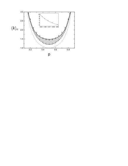
Figure 7: Phase diagram for undirected RBN model in classical random graphs. Dotted line is a solution of basic Eq. (19). Filled points represent numerical simulations made for the whole network (the same data are shown in Fig. 5). Open points and dashed line correspond respectively to numerical simulations and analytic prediction of Eq. (42) for the Kauffman model defined in giant components only. Solid line is the solution of final eq. (47). Gray area emphasizes the set of parameters where the chaotic behavior, although present in the giant component, is not yet visible in the whole network.

It is easy to check, that in the simplest case of classical random graphs the parameter $w^{*}(k)$ (43) is given by

$$w^{*}(k)=\frac{1-u-u^{k-1}+u^{k+u-1}}{(1-u)(1-u^{k})}.$$ (44)

Inserting the last formula into (42), and then numerically solving the resulting equation for $\langle k\rangle$ we obtain theoretical prediction for the critical line of the Kauffman model in giant components of these graphs. In Fig. 7 one can see that numerical simulations quite tally with the theoretical prediction of Eq. (42). Given the figure, we would also like to take note of two other interesting effects related to the analyzed problem. First, the critical line characterizing the giant component significantly differs from the curve described by the formula (18). It is shifted towards the numerically obtained critical line characterizing the whole network. The observation is in some sense promising, as it partially confirms the main proposition of this paper, which states that the percolation transition is responsible for discrepancies observed in Fig. 5. The second effect concerns mutual relationship between the behavior of the giant component and the behavior of the whole network. Since one knows that the giant component makes up a macroscopic part of the network (it grows linearly with the network size $N$, and becomes infinite in the thermodynamic limit $N\rightarrow\infty$) one could expect that dynamics of the whole network should reflect behavior of the giant component. Thus, the question is, why the numerically obtained critical line characterizing the whole network differs from the theoretical prediction for the giant component. In other words, why, for the set of parameters marked by the light gray area in Fig. 7, the chaotic behavior of the giant component is not visible in the whole network.

To solve the problem stated at the end of the last paragraph, let us briefly recall what the numerical simulations of the Kauffman model consist in. Thus, in numerical studies we check how the initial perturbation of the system $x(0)\equiv 1-\Delta$ (5), where $\Delta\ll 1$, develops over time. In general, when the parameter $x(t=T)<x(0)$ we identify the system as the chaotic one. On the other hand, when $x(0)\leq x(t=T)\leq 1$ we treat it as being in the ordered phase. In reality, however, due to the fact that in the vicinity of the percolation transition the considered Kauffman networks are strongly heterogenous, they consist of the giant component which is escorted by a number of small tree-like clusters and isolated nodes, the systems should by treated more carefully.

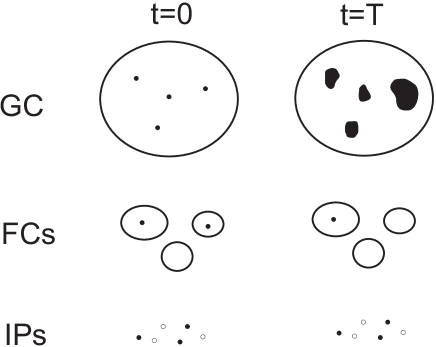
Figure 8: Schematic plot of spreading of perturbation in giant component (GC), finite clusters (FCs) and isolated points (IPs). In GC damage spreads, in FCs it shrinks, while in IPs it does not change.

To better describe the situation let us choose the system parameters from the region that is marked by the light gray color in Fig. 7. Then, we introduce a quantity $\Omega$, which measures chaoticity in the system as a mean damage size caused by a single node perturbation. If $\Omega>(<)0$ then mean damage size grows(shrinks) in time. Condition $\Omega=0$ will allow us to derive the relation for the critical line in the whole network.

Let us now divide the network into three parts: giant connected component (GC), finite clusters (FCs) and isolated points (IPs). The figure 8 shows schematically how the single node perturbation evolves in time in these three parts of the network. In studied range of parameters the giant component behaves chaotically, i.e. the mean damage size is larger than initial perturbation and $\Omega_{GC}>0$. On the other hand, the small density of connections in finite tree-like clusters does not allow perturbation to spread out and $\Omega_{FCs}<0$. Because the state of isolated nodes does not change in time, then $\Omega_{IPs}=0$. Now, if one perturb randomly a set of nodes in the whole network, fraction $S$ of perturbations will be located in GC, fraction $(1-S)(1-P(k=0))$ will be located in FCs, and the rest of them, i.e. $(1-S)P(k=0)$ will perturb isolated nodes. Now one can write the condition for transition from the frozen to the chaotic state in the whole network:

$$S\Omega_{GC}+(1-S)(1-P(k=0))\Omega_{FCs}=0,$$ (45)

where $\Omega$, $P(k)$ and $S$ depend on $\langle k\rangle$. This equation shows that the ordered behavior of small clusters can shield the chaotic behavior of the giant component. Only when chaoticity in GC is sufficiently developed, this shielding effect becomes neglected.

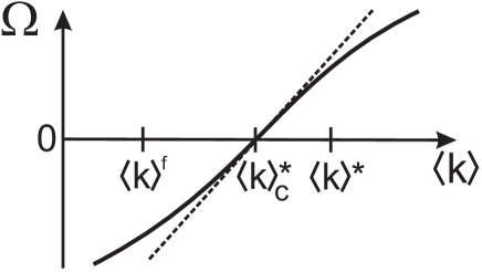
Figure 9: Chaoticity $\Omega$ (solid line) in the viciity of the critical point $\langle k\rangle^{*}_{c}$. $\langle k\rangle^{*}$ and $\langle k\rangle^{f}$ are the average node degree in GC and in FCs respectively. Dashed line presents linear approximation of $\Omega$.

Now, expanding $\Omega$ into power series at $\langle k\rangle=\langle k\rangle_{c}$

$$\Omega=\Omega_{0}+\frac{\partial\Omega}{\partial\langle k\rangle}(\langle k\rangle-\langle k\rangle_{c}),$$ (46)

where $\Omega_{0}=0$ in critical point (cf. Fig. 9), one gets the final equation for the critical line:

$$S(\langle k\rangle^{*}-\langle k\rangle^{*}_{c})=(S-1)(1-P(k=0))(\langle k\rangle^{f}-\langle k\rangle^{*}_{c}),$$ (47)

where $\langle k\rangle^{f}=\langle k\rangle u$ (cf. eq.(25) in [25]). The numerical solution of this implicit equation is presented in Fig. 7 as the solid line.

5 Conclusions

This study was done to investigate the properties of undirected KBN model in the vicinity of percolation threshold. We derived a mean field formula for the critical line characterizing KBN model in undirected and uncorrelated random graphs with arbitrary degree distributions. We have shown that the results of classical mean field theory differ from these obtained by numerical simulations. We have shown also that, to explain the discrepancies one has to take into account the effect of correlations between adjoining nodes in the giant connected component as well as the effect of shielding by finite size clusters. As one can see the problem is not easy even for undirected networks. As we have shown in figure 1 and 2 a directedness of the network introduces further complications into calculations. Nevertheless, we think that a similar approach can be derived even for that case. We hope that the presented work will encourage others to pursue these topics in the near future.

6 Acknowledgments

The work was funded in part by the European Commission Project CREEN FP6-2003-NEST-Path-012864 (P.F.), and by the Ministry of Education and Science in Poland under Grant 134/E-365/6.PR UE/DIE 239/2005-2007 (A.F.).

References

References

- [1] S. A. Kauffman, J. Theor. Biol. 22, 437 (1969).
- [2] S. Huang and D. E. Ingber, Exp. Cell Res. 261, 91 (2000).
- [3] S. A. Kauffman and E. D. Weinberger, J. Theor. Biol. 141, 211 (1989).
- [4] S. Bornholdt and K. Sneppen, Proc. Royal Soc. Lond. B 266, 2281 (2000).
- [5] R. Lambiotte, S. Thurner, and R. Hanel, physics/0612025 (2006).
- [6] L. Wang, E. E. Pichler and J. Ross, Proc. Natl. Acad. Sci. 87, 9467 (1990).
- [7] C. F. Baillie and D. A. Johnston, Phys. Lett. B 326, 51 (1994).
- [8] S. A. Kauffman, Physica D 42, 135 (1990).
- [9] R. V. Sole and J. M. Montoya, Proc. Royal Soc. Lond. B 268, 2039 (2001).
- [10] D. Stauffer, J. Stat. Phys. 74, 1293 (1994).
- [11] R. Albert and A. L. Barabasi, Rev. Modern Phys. 74, 47 (2002).
- [12] A. L. Barabasi, Linked: The New Science of Networks, Perseus Publishing, Cambridge, MA, 2002.
- [13] B. Derrida and Y. Pomeau, Europhys. Lett. 1, 45 (1986).
- [14] B. Luque and R. V. Sole, Phys. Rev. E 55, 257 (1997).
- [15] M. Aldana, Physica D 185, 45 (2003).
- [16] M. Aldana and P. Cluzel, Proc. Natl. Acad. Sci. 100, 8710 (2003).
- [17] D. Lee and H. Rieger, cond-mat/0605730 (2006).
- [18] M. Boguna, priv. comm. (2007).
- [19] T. Rohlf, N. Gulbahce, and C. Teuscher, cond-mat/0701601 (2007).
- [20] P. Ramo, J. Kesseli, and O. Yli-Harja, J. Theor. Biol. 242, 164 (2006).
- [21] M. E. J. Newman, Phys. Rev. Lett. 89, 208701 (2002).
- [22] J. D. Noh, arxiv:0705.0087 (2007).
- [23] M. E. J. Newman, S. H. Strogatz, and D. J. Watts, Phys. Rev. E 64, 026118 (2001).
- [24] M. N. Barber, ”Finite-size Scaling”, in C. Domb and J. L. Lebowitz, it Phase Transitions and Critical Phenomena, Vol. 8, Academic Press, 146-268 (1983).
- [25] P. Bialas and A. Oles, arxiv:0710.3319 (2007).
- [26] S. N. Dorogovtsev, J. F. F. Mendes, and A. N. Samukhin, Phys. Rev. E 64, 025101(R) (2001).
- [27] N. Schwartz, R. Cohen, D. ben-Avraham, A.-L. Barabasi, and S. Havlin, Phys. Rev. E 66, 015104(R) (2002).
- [28] S. N. Dorogovtsev, A. V. Goltsev, and J. F. F. Mendes, arXiv:0705.0010.
- [29] R. Albert, H. Jeong, and A.-L. Barabasi, Nature 406, 378 (2000).
- [30] R. Cohen, K. Erez, D. ben-Avraham, and S. Havlin, Phys. Rev. Lett. 85, 4626 (2000).
- [31] P. Fronczak, A. Fronczak, and J. A. Holyst, arxiv:0707.1963v2 (2007).
- [32] M. Molloy and B. Reed, Ran. Struct. and Algor. 6, 161 (1995).
- [33] M. Boguna and R. Pastor-Satorras, Phys. Rev. E 68, 036112 (2003).