Quasi-particle propagation in quantum Hall systems

Abstract

We study various geometrical aspects of the propagation of particles obeying fractional statistics in the physical setting of the quantum Hall system. We find a discrete set of zeros for the two-particle kernel in the lowest Landau level; these arise from a combination of a two-particle Aharonov-Bohm effect and the exchange phase related to fractional statistics. The kernel also shows short distance exclusion statistics, for instance, in a power law behavior as a function of initial and final positions of the particles. We employ the one-particle kernel to compute impurity-mediated tunneling amplitudes between different edges of a finite-sized quantum Hall system and and find that they vanishes for certain strengths and locations of the impurity scattering potentials. We show that even in the absence of scattering, the correlation functions between different edges exhibits unusual features for a narrow enough Hall bar.

I Introduction

Fractional statistics in two dimensions leinaas ; wilczek1 has been studied extensively ever since it was proposed that quasi-particles in fractional quantum Hall systems carry this attribute. laughlin1 ; laughlin2 ; halperin ; arovas ; jain1 Such particles are called anyons; the wave function of two or more such particles picks up a phase (which may be different from $\pm 1$) when any two of them are exchanged. Interest in this subject has grown further in recent years due to the possibility of topological quantum computation kitaev1 and the development of spin models which support anyonic excitations kitaev2 ; pachos ; han ; chen . Several proposals kivelson ; jain2 ; chamon1 ; isakov ; safi ; kane1 ; vishveshwara1 ; kim ; grosfeld ; law1 ; braggio ; feldman and experimental attempts camino have been made to detect the fractional statistics of quasi-particles in fractional quantum Hall systems. (Here we restrict our attention to Abelian fractional statistics). While there are many studies of anyons propagating at the edges of fractional quantum Hall systems wen1 , anyon correlations in the bulk have not been studied in as much detail martin . Since anyons are intrinsically two-dimensional objects, a coherent understanding of their behavior necessitates a study of their properties in the bulk. Here we undertake such a study of the bulk properties of anyons in the lowest Landau level of a quantum Hall system.

Given that fractional statistics is an intrinsically two-particle concept, the most direct way of understanding anyonic behavior is by investigating the properties of the two-particle kernel. Historically, two-particle kernels have played an important role in many areas of physics including scattering problems in particle physics, quantum optics and astrophysics baym ; hbt . In particular, seminal work by Hanbury Brown and Twiss showed that bosons tend to ‘bunch’ when arriving at a given point in space-time. Fermions, on the other hand, tend to ‘anti-bunch’. Two-particle kernels are in fact key for studying the effects of quantum statistics on correlations between two identical particles which are propagating together. The one-particle kernel is also useful to study even though it is not directly affected by the exchange phase; for instance, it provides information about the charge of the particle (if one considers its motion in a magnetic field) and tunneling between different edges of a quantum Hall system. Moreover, as elucidated in what follows, information on exchange statistics can also be derived by analyzing the extent to which two-particle properties can be decomposed into single-particle properties.

In this paper, we analyze several aspects of the propagation of anyons through the bulk of a quantum Hall system in the presence of a strong magnetic field. In particular, we show that the simultaneous propagation of two anyons in the lowest Landau level exhibits some surprising features depending on the geometrical arrangement of the initial and final positions. These arise from an interplay of the Aharonov-Bohm phase due to the magnetic field and the phase due to the exchange of two anyons. We discuss a physical realization of these anyon trajectories. As a first step towards connecting bulk physics to the boundary of the quantum Hall system, as is relevant to any physical situation, we then analyze single-particle properties in a bounded system. We discuss some unusual features which can arise when a single particle propagates from one edge to another through the bulk of a quantum Hall system which has the form of a narrow strip.

The plan of this paper is as follows. In Sec. II, we discuss the one-particle kernel of a charged particle moving in a magnetic field. This will be used later to compute the two-particle kernel (using centre of mass and relative coordinates) and the amplitude for tunneling across a narrow quantum Hall system. In Sec. III, we calculate the two-particle kernel for fermions, bosons and anyons in general. We show that the two-anyon kernel in the lowest Landau level vanishes if the initial and final positions satisfy a special set of conditions. These conditions can be given a simple interpretation in terms of the phase difference of two paths. We propose some experiments for using the two-anyon kernel to measure their charge and exchange statistics. The possible corrections arising from higher Landau levels are also discussed. In Sec. IV, we consider tunneling of a particle between different edges of a quantum Hall strip; the tunneling is induced by impurities which may be present anywhere in the strip. We show that the tunneling amplitude vanishes if the strengths and locations of the impurities satisfy certain conditions. We propose a Hall bar geometry for observing these effects. In Sec. V, we study two-point correlators along different edges of a quantum Hall system. Once again, we find that the correlator can vanish if the system has the form of a narrow strip, and the two points are separated by some particular distances. We summarize our results in Sec. VI. A condensed version of this work has appeared earlier vishveshwara2 .

In the discussions to follow, various correlators are analyzed depending on the properties in question. We clarify their definitions at the outset: since we will discuss several correlators in this paper, it may be useful to list them here. In Secs. II and III, we will discuss the one- and two-particle kernels. The one-particle kernel $K_{1}({\vec{r}}_{f};{\vec{r}}_{i};t)$ is the amplitude for a particle to go from an initial position ${\vec{r}}_{i}$ to a final position ${\vec{r}}_{f}$ in time $t$, where $t>0$. We define the kernel to be zero if $t<0$. Given a vacuum state $|0\rangle$, and a second quantized field $\Psi({\vec{r}},t)$ which annihilates a particle at $({\vec{r}},t)$, the kernel is given by

$$K_{1}({\vec{r}}_{f};{\vec{r}}_{i};t) = \langle 0|\Psi({\vec{r}}_{f},t)\Psi^{\dagger}({\vec{r}}_{i},0)|0\rangle$$ (1)

$$= \sum_{n}~{}\psi_{n}({\vec{r}}_{f})~{}\psi_{n}^{*}({\vec{r}}_{i})~{}e^{-iE_{n}t/\hbar},$$

where $E_{n}$ and $\psi_{n}$ in the second line denote the eigenvalues and eigenfunctions respectively of the one-particle Hamiltonian, and we have assumed the label $n$ to be discrete. The Fourier transform of this kernel is given by

$${\tilde{K}}_{1}({\vec{r}}_{f};{\vec{r}}_{i};E) = \int_{0}^{\infty}~{}dt~{}K_{1}({\vec{r}}_{f};{\vec{r}}_{i};t)~{}e^{iEt/\hbar}$$ (2)

$$= -i\hbar~{}\sum_{n}~{}\frac{\psi_{n}({\vec{r}}_{f})\psi_{n}^{*}({\vec{r}}_{i})}{E_{n}-E-i\epsilon}.$$

The two-particle kernel is defined in an analogous way. In Sec. IV, we will use the retarded Green’s function; this is related to the one-particle kernel as $G({\vec{r}}_{f};{\vec{r}}_{i};E)=(i/\hbar){\tilde{K}}_{1}({\vec{r}}_{f};{\vec{r}}_{i};E)$. Finally, in Sec. V, we will discuss a two-point correlator. Given the ground state $|G\rangle$ of a system of several non-interacting electrons in which all states up to a Fermi energy $E_{F}$ are filled (the case of interest in Sec. V), we will be interested in the correlator

$$C({\vec{r}}_{1};{\vec{r}}_{2};t) = \langle G|\Psi^{\dagger}({\vec{r}}_{1},0)\Psi({\vec{r}}_{2},t)|G\rangle$$ (3)

$$= \sum_{E_{n}<E_{F}}~{}\psi_{n}^{*}({\vec{r}}_{1})~{}\psi_{n}({\vec{r}}_{2})~{}e^{-iE_{n}t/\hbar}.$$

Note that Eqs. (1) and (3) differ in the range of values of $n$ which is summed over.

II One-particle kernel

For a free particle moving in two dimensions, say the $x-y$ plane, the one-particle kernel is given by

$$K_{1}({\vec{r}}_{f};{\vec{r}}_{i};t)~{}=~{}\frac{\mu}{i2\pi\hbar t}~{}e^{i\mu({\vec{r}}_{f}-{\vec{r}}_{i})^{2}/(2\hbar t)},$$ (4)

where $\mu$ is the mass of the particle.

Let us now consider the effect of a uniform magnetic field ${\vec{B}}=B{\hat{z}}$ applied perpendicular to the $x-y$ plane. If we use the symmetric gauge ${\vec{A}}=(1/2){\vec{B}}\times{\vec{r}}$, the Hamiltonian is given by

$$H~{}=~{}\frac{1}{2\mu}~{}(p_{x}+\frac{eB}{2c}y)^{2}~{}+~{}\frac{1}{2\mu}~{}(p_{y}-\frac{eB}{2c}x)^{2},$$ (5)

where $e$ and $c$ denote the charge of the particle and the speed of light respectively. For convenience, we assume that $eB>0$. The cyclotron frequency is given by $\omega_{c}=eB/\mu c$. As shown in Appendix A, the kernel is given by

$$K_{1}({\vec{r}}_{f};{\vec{r}}_{i};t)$$

$$=~{}\frac{eB}{i4\pi\hbar c\sin(\omega_{c}t/2)}~{}\exp[~{}\frac{ieB\cot(\omega_{c}t/2)}{4\hbar c}~{}({\vec{r}}_{f}-{\vec{r}}_{i})^{2}$$

$$~{}~{}~{}~{}~{}~{}~{}~{}~{}~{}~{}~{}~{}~{}~{}~{}~{}~{}~{}~{}~{}~{}~{}~{}~{}~{}~{}~{}~{}~{}~{}+~{}\frac{ieB}{2\hbar c}~{}{\hat{z}}\cdot{\vec{r}}_{i}\times{\vec{r}}_{f}~{}].$$ (6)

Eq. (6) can be written in imaginary time by replacing $t$ by $-i\tau$. We then obtain

$$K_{1}({\vec{r}}_{f};{\vec{r}}_{i};\tau)$$

$$=\frac{eB}{4\pi\hbar c\sinh(\omega_{c}\tau/2)}~{}\exp[-~{}\frac{eB\coth(\omega_{c}\tau/2)}{4\hbar c}({\vec{r}}_{f}-{\vec{r}}_{i})^{2}$$

$$~{}~{}~{}~{}~{}~{}~{}~{}~{}~{}~{}~{}~{}~{}~{}~{}~{}~{}~{}~{}~{}~{}~{}~{}~{}~{}~{}~{}~{}~{}~{}+~{}\frac{ieB}{2\hbar c}~{}{\hat{z}}\cdot{\vec{r}}_{i}\times{\vec{r}}_{f}].$$ (7)

The kernel in the lowest Landau level (LLL) can be obtained by multiplying Eq. (7) by $e^{\omega_{c}\tau/2}$ (this is equivalent to shifting all the energy levels by $\hbar\omega_{c}/2$ in order to make the ground state energy zero), and then letting $\tau\to\infty$,

$$K_{1}({\vec{r}}_{f};{\vec{r}}_{i}) = \frac{eB}{2\pi\hbar c}~{}\exp[-~{}\frac{eB}{4\hbar c}~{}({\vec{r}}_{f}-{\vec{r}}_{i})^{2}$$ (8)

$$~{}~{}~{}~{}~{}~{}~{}~{}~{}~{}~{}~{}~{}+~{}\frac{ieB}{2\hbar c}~{}{\hat{z}}\cdot{\vec{r}}_{i}\times{\vec{r}}_{f}].$$

Absorbing a factor of the Landau length $l=\sqrt{{\hbar c}/eB}$ in the coordinates ${\vec{r}}_{i}$ and ${\vec{r}}_{f}$, we have

$$K_{1}({\vec{r}}_{f};{\vec{r}}_{i}) = \frac{1}{2\pi l^{2}}~{}\exp[-\frac{1}{4}~{}({\vec{r}}_{f}-{\vec{r}}_{i})^{2}+\frac{i}{2}{\hat{z}}\cdot{\vec{r}}_{i}\times{\vec{r}}_{f}],$$

where the positions ${\vec{r}}_{i}$ are now dimensionless quantities. We rewrite Eq. (LABEL:k1mag4) using complex coordinates, $z=x+iy$ and $z^{*}=x-iy$. We then obtain

$$K_{1}({\vec{r}}_{f};{\vec{r}}_{i}) = \frac{1}{2\pi l^{2}}~{}\exp[-\frac{1}{4}~{}(|z_{f}|^{2}+|z_{i}|^{2})~{}+~{}\frac{1}{2}z_{f}z_{i}^{*}].$$

Eq. (LABEL:k1mag5) can be derived in a different way. In general, the kernel is given by a sum over all the eigenstates of the Hamiltonian $H$,

$$K_{1}({\vec{r}}_{f};{\vec{r}}_{i};\tau)~{}=~{}\sum_{n}~{}\psi_{n}({\vec{r}}_{f})~{}\psi_{n}^{*}({\vec{r}}_{i})~{}e^{-E_{n}\tau/\hbar}.$$ (11)

The Hamiltonian in Eq. (5) written in dimensionless complex coordinates takes the form

$$H~{}=~{}\hbar\omega_{c}~{}[-~{}2\frac{\partial}{\partial z}\frac{\partial}{\partial z^{*}}~{}+~{}\frac{1}{8}zz^{*}~{}-~{}\frac{z}{2}\frac{\partial}{\partial z}~{}+~{}\frac{z^{*}}{2}\frac{\partial}{\partial z^{*}}].$$ (12)

Assuming that the eigenstates of $H$ are of the form $\psi=f(z,z^{*})\exp(-|z|^{2}/4)$, we obtain the eigenvalue equation ${\tilde{H}}f=Ef$, where

$${\tilde{H}}~{}=~{}\hbar\omega_{c}~{}[-~{}2\frac{\partial}{\partial z}\frac{\partial}{\partial z^{*}}~{}+~{}z^{*}\frac{\partial}{\partial z^{*}}~{}+~{}\frac{1}{2}~{}].$$ (13)

The ground states of $\tilde{H}$ are given by analytic functions of $z$. The normalized wave functions in the LLL are given by

$$\psi_{n}({\vec{r}})~{}=~{}\frac{1}{l\sqrt{n!~{}2\pi}}~{}\left(\frac{z}{\sqrt{2}}\right)^{n}~{}\exp[-\frac{1}{4}~{}|z|^{2}],$$ (14)

where $n=0,1,2,\cdots$. For large values of $n$, the probability corresponding to the $n^{\rm th}$ wave function is peaked on a circle of radius $l\sqrt{2n}$. Substituting Eq. (14) in Eq. (11) and letting $\tau\to\infty$, we obtain the expression in Eq. (LABEL:k1mag5); recall that we have shifted the energy levels so that $E_{n}=0$.

The kernel in Eq. (LABEL:k1mag5) satisfies the reproducing property

$$\psi({\vec{r}}_{f})~{}=~{}\int~{}d^{2}{\vec{r}}_{i}~{}K_{1}({\vec{r}}_{f};{\vec{r}}_{i})~{}\psi({\vec{r}}_{i}).$$ (15)

A simple way to prove this is to note that an arbitrary wave function $\psi$ in the LLL can be written as

$$\psi({\vec{r}})~{}=~{}\sum_{n=0}^{\infty}~{}c_{n}z^{n}\exp[-\frac{1}{4}|z|^{2}],$$ (16)

where the $c_{n}$’s can take any values, and then show that the reproducing property holds for each term $z^{n}$ separately.

III Two-particle kernel

III.1 Fermions and bosons

For two identical fermions, it is well-known that the scattering amplitude is zero if the scattering angle $\theta$ is equal to $\pi/2$. shankar ; gasiorowicz This is because of the antisymmetry of the wave function of two identical fermions. If the scattering amplitude for one permutation of the initial particles going to the final particles is given by $f(\theta)$, then the amplitude for the other permutation is given by $-f(\pi-\theta)$. The total amplitude given by $f(\theta)-f(\pi-\theta)$ vanishes for $\theta=\pi/2$, no matter what the form of the function $f(\theta)$ is. For two identical anyons (the precise definition of anyons will be given in Sec. III.2), it is known that the scattering amplitude is not zero for any value of $\theta$, except of course for the special case in which the anyons are fermions. law2

The above statements are usually made in the context of asymptotic states where the initial and final particles are very far away from each other. However, we can use the two-particle kernel to study what happens when the particle positions are not far from each other. Let $K_{2}({\vec{r}}_{1f},{\vec{r}}_{2f},{\vec{r}}_{1i},{\vec{r}}_{2i};t)$ denote the amplitude for two identical particles going from the initial positions ${\vec{r}}_{1i},{\vec{r}}_{2i}$ to the final positions ${\vec{r}}_{1f},{\vec{r}}_{2f}$ in time $t$. For non-interacting particles, $K_{2}$ can be written in terms of the one-particle kernel $K_{1}$. Namely,

$$K_{2}({\vec{r}}_{1f},{\vec{r}}_{2f};{\vec{r}}_{1i},{\vec{r}}_{2i};t)$$

$$=~{}K_{1}({\vec{r}}_{1f};{\vec{r}}_{1i};t)~{}K_{1}({\vec{r}}_{2f},{\vec{r}}_{2i};t)$$

$$~{}~{}~{}\mp~{}K_{1}({\vec{r}}_{2f};{\vec{r}}_{1i};t)~{}K_{1}({\vec{r}}_{1f},{\vec{r}}_{2i};t),$$ (17)

where the upper and lower signs are for fermions and bosons respectively; in a second quantized formalism, Eq. (17) follows from Wick’s theorem. fetter Using Eq. (4), we find that the two-particle kernel is zero for two fermions for arbitrary values of $t$ if and only if

$$({\vec{r}}_{1i}-{\vec{r}}_{2i})\cdot({\vec{r}}_{1f}-{\vec{r}}_{2f})=0,$$ (18)

namely, the initial and final relative positions of the two particles are perpendicular to each other. For bosons, there is no choice of initial and final positions for which the two-particle kernel is zero for arbitrary values of $t$.

The situation changes in an interesting way in the presence of a magnetic field if the particles are charged. Substituting Eq. (6) in Eq. (17), we find that the two-particle kernel vanishes only if Eq. (18) is satisfied, and

$$\frac{eB}{2\hbar c}~{}{\hat{z}}\cdot({\vec{r}}_{1i}-{\vec{r}}_{2i})\times({\vec{r}}_{1f}-{\vec{r}}_{2f})$$

$$=~{}2n\pi\quad{\rm for~{}~{}fermions},$$

$$=~{}(2n+1)\pi\quad{\rm for~{}~{}bosons},$$ (19)

where $n=0,\pm 1,\pm 2,\cdots$.

It is instructive to understand the conditions in Eqs. (18-19) from a path integral point of view. Consider some configurations of initial and final positions shown in Fig. 1. The two-particle kernel in Eq. (17) is a sum over all paths belonging to one of two types: paths of type $I$ are those in which one particle goes from ${\vec{r}}_{1i}$ to ${\vec{r}}_{1f}$ and the other goes from ${\vec{r}}_{2i}$ to ${\vec{r}}_{2f}$, while paths of type $II$ are those in which one particle goes from ${\vec{r}}_{1i}$ to ${\vec{r}}_{2f}$ and the other goes from ${\vec{r}}_{2i}$ to ${\vec{r}}_{1f}$. We see from Eq. (LABEL:k1mag5) that the magnitudes of the kernels along paths of types $I$ and $II$ are given by

$$\exp~{}[-\frac{1}{4}~{}(|z_{1f}-z_{1i}|^{2}~{}+~{}|z_{2f}-z_{2i}|^{2})]$$

$${\rm and} \exp~{}[-\frac{1}{4}~{}(|z_{1f}-z_{2i}|^{2}~{}-~{}|z_{2f}-z_{1i}|^{2})]$$ (20)

respectively. If these two magnitudes are not equal, then the corresponding kernels cannot add up to zero no matter what their phases are. The condition that the magnitudes in Eq. (20) should be equal implies that $(z_{1f}-z_{2f})(z_{1i}^{*}-z_{2i}^{*})$ is imaginary; this is equivalent to the perpendicularity condition in Eq. (18). Next, we look at the phases of the kernels corresponding to paths $I$ and $II$. The difference of the phases of the two kernels is described by Eq. (19) as follows. We observe that

$$\frac{1}{2}~{}{\hat{z}}\cdot({\vec{r}}_{1i}\times{\vec{r}}_{1f}~{}+~{}{\vec{r}}_{1f}\times{\vec{r}}_{2i}~{}+~{}{\vec{r}}_{2i}\times{\vec{r}}_{2f}~{}+~{}{\vec{r}}_{2f}\times{\vec{r}}_{1i})$$ (21)

is the area enclosed by a closed loop formed by moving in straight lines from ${\vec{r}}_{1i}$ to ${\vec{r}}_{1f}$ to ${\vec{r}}_{2i}$ to ${\vec{r}}_{2f}$ and back to ${\vec{r}}_{1i}$; the area is taken to be positive for an anticlockwise loop. The left hand side of Eq. (19) can then be interpreted as the Aharonov-Bohm phase for a particle going around the above loop. The total phase difference between paths of types $I$ and $II$ is given by the sum of the Aharonov-Bohm phase in Eq. (19), and a phase due to an anticlockwise exchange of the two particles which is given by $\pi$ and $0$ for fermions and bosons respectively. (For fermions and bosons, the exchange phase modulo $2\pi$ is the same for clockwise and anticlockwise exchanges, but for anyons the two phases differ). The two-particle kernel vanishes if the phases of paths $I$ and $II$ differ by $\pi$. Eq. (19) then follows in a straightforward way.

Figure 1: Two representative configurations for anyons starting at points $\vec{r}_{1i}$ and $\vec{r}_{2i}$ to end at points $\vec{r}_{1f}$ and $\vec{r}_{2f}$. As the particles are indistinguishable, it is not possible to determine which of two possible paths $I$ and $II$ each particle takes.

To summarize, the two-particle kernel in a magnetic field vanishes if the initial and final relative positions are mutually perpendicular, and if the area of the loop takes a discrete set of values which depends on the statistics of the particles. This may be called a two-particle Aharonov-Bohm effect buttiker1 ; buttiker2 ; such an effect has been observed recently for two fermions neder .

Looking at Eqs. (6) and (8), we see that the condition for the vanishing of the two-particle kernel is given by Eqs. (18) and (19), whether one considers all the states in a magnetic field or only the states in the LLL. For the general case of anyons, we will find the condition for the vanishing of the two-particle kernel in the LLL in the next section; the corresponding condition for all states in a magnetic field is not yet known for anyons.

It is useful to derive the two-particle kernel for fermions and bosons in a different way, using center of mass and relative coordinates; this can then be generalized to find the kernel for two anyons. We define the center of mass coordinate ${\vec{R}}=({\vec{r}}_{1}+{\vec{r}}_{2})/2$, momentum ${\vec{P}}={\vec{p}}_{1}+{\vec{p}}_{2}$, mass $2\mu$ and charge $Q=2e$, and the relative coordinate ${\vec{r}}={\vec{r}}_{1}-{\vec{r}}_{2}$, momentum ${\vec{p}}=({\vec{p}}_{1}-{\vec{p}}_{2})/2$, mass $\mu/2$ and charge $q=e/2$. The Hamiltonian then decouples as

$$H = \frac{1}{4\mu}~{}(P_{x}+\frac{QB}{2c}Y)^{2}~{}+~{}\frac{1}{4\mu}~{}(P_{y}-\frac{QB}{2c}X)^{2}$$ (22)

$$+~{}\frac{1}{\mu}~{}(p_{x}+\frac{qB}{2c}y)^{2}~{}+~{}\frac{1}{\mu}~{}(p_{y}-\frac{qB}{2c}x)^{2}.$$

The eigenstates of this Hamiltonian are given by products of eigenstates of the center of mass and relative coordinate systems, and the energies are given by sums of the individual energies. In the LLL, the eigenstates of the centre of mass system are given by

$$\psi_{n}({\vec{R}})=\sqrt{\frac{QB}{n!~{}2\pi\hbar c}}\left(Z\sqrt{\frac{QB}{2\hbar c}}\right)^{n}~{}\exp[-\frac{QB}{4\hbar c}~{}|Z|^{2}],$$ (23)

where $Z=X+iY$, and $n=0,1,2,\cdots$. The eigenstates of the relative system are given by

$$\psi_{p}({\vec{r}})=\sqrt{\frac{qB}{p!~{}2\pi\hbar c}}\left(z\sqrt{\frac{qB}{2\hbar c}}\right)^{p}~{}\exp[-\frac{qB}{4\hbar c}~{}|z|^{2}],$$ (24)

where $p=0,2,4,\cdots$ for bosons and $1,3,5,\cdots$ for fermions. The condition on $p$ arises from the fact that the wave functions must be symmetric (antisymmetric) under the exchange of the two particles, $z\to-z$, for bosons and fermions respectively.

The two-particle kernel in imaginary time is given by

$$K_{2}({\vec{r}}_{1f},{\vec{r}}_{2f};{\vec{r}}_{1i},{\vec{r}}_{2i};\tau)$$

$$=~{}\sum_{n}~{}\psi_{n}({\vec{R}}_{f})~{}\psi_{n}^{*}({\vec{R}}_{i})~{}e^{-E_{n}\tau/\hbar}$$

$$~{}~{}~{}~{}\times~{}\sum_{p}~{}\psi_{p}({\vec{r}}_{f})~{}\psi_{p}^{*}({\vec{r}}_{i})~{}e^{-E_{p}\tau/\hbar}.$$ (25)

Absorbing the Landau length in the length scale and shifting the ground state energy to zero as before, we find that the kernel in the LLL is given by

$$K_{2}({\vec{r}}_{1f},{\vec{r}}_{2f};{\vec{r}}_{1i},{\vec{r}}_{2i})$$

$$=~{}\frac{1}{(2\pi l^{2})^{2}}~{}\exp~{}[-\frac{1}{4}(|z_{1f}|^{2}+|z_{2f}|^{2}+|z_{1i}|^{2}+|z_{2i}|^{2})$$

$$~{}~{}~{}~{}~{}~{}~{}~{}~{}~{}~{}~{}~{}~{}~{}~{}~{}~{}~{}~{}+\frac{1}{4}(z_{1f}+z_{2f})(z_{1i}^{*}+z_{2i}^{*})]$$

$$\times~{}\sinh[\frac{1}{4}(z_{1f}-z_{2f})(z_{1i}^{*}-z_{2i}^{*})]\quad{\rm for~{}~{}fermions},$$

$$\times~{}\cosh[\frac{1}{4}(z_{1f}-z_{2f})(z_{1i}^{*}-z_{2i}^{*})]\quad{\rm for~{}~{}bosons}.$$ (26)

One can check that Eq. (26) agrees with the results obtained by combining Eqs. (LABEL:k1mag5) and (17).

The kernel in Eq. (26) satisfies the reproducing property

$$\psi({\vec{r}}_{1f},{\vec{r}}_{2f}) = \int~{}d^{2}{\vec{r}}_{1i}~{}d^{2}{\vec{r}}_{2i}~{}K_{2}({\vec{r}}_{1f},{\vec{r}}_{2f};{\vec{r}}_{1i},{\vec{r}}_{2i})$$ (27)

$$~{}~{}~{}~{}\times~{}\psi({\vec{r}}_{1i},{\vec{r}}_{2i}).$$

This can be shown by noting that an arbitrary antisymmetric (symmetric) two-particle wave function $\psi$ in the LLL can be written as

$$\psi({\vec{r}}_{1},{\vec{r}}_{2}) = \sum_{n,p=0}^{\infty}~{}c_{n,p}~{}(z_{1}+z_{2})^{n}~{}(z_{1}-z_{2})^{p}$$ (28)

$$~{}~{}~{}~{}\times~{}\exp[-\frac{1}{4}(|z_{1}|^{2}+|z_{2}|^{2})],$$

where $p$ is restricted to odd (even) integers for fermions (bosons) respectively, and then proving that the reproducing property holds for each term $(z_{1}+z_{2})^{n}~{}(z_{1}-z_{2})^{p}$ separately.

III.2 Anyons in the lowest Landau level

We will now derive the two-particle kernel for anyons in the LLL. Anyons are particles living in two dimensions with the property that when two of them are interchanged in an anticlockwise (clockwise) direction, the wave function picks up a phase of $e^{i\pi\alpha}$ ($e^{-i\pi\alpha}$) respectively; here $\alpha$ is a real parameter lying in the range $-1<\alpha\leq 1$. leinaas ; wilczek1 (Bosons and fermions correspond to the special cases $\alpha=0$ and 1 respectively). For instance, for a system of two particles, we demand that if we continuously vary the arguments ${\vec{r}}_{1}$ and ${\vec{r}}_{2}$ of a wave function so as to interchange them in an anticlockwise sense (without ever making them equal to each other), the final wave function must be $e^{i\pi\alpha}$ times the initial wave function. These statements are true in a formalism in which the Hamiltonian does not explicitly depend on $\alpha$, but the wave functions are multi-valued. There is an alternative formalism in which the Hamiltonian depends on $\alpha$, and the wave functions are single-valued. A brief discussion of these two approaches is given in Appendix B. Further details can be found in Refs. wilczek2, ; forte, ; lerda, ; khare, ; myrheim, .

In a fractional quantum Hall system with filling fraction given by $1/m$, where $m$ is an odd integer, the quasi-particles are believed to behave as anyons. The charge of a quasi-hole (quasi-electron) is $-e/m$ ($e/m$), where $e$ is the charge of an electron, and these are anyons with $\alpha=1/m~{}$ ($-1/m$) respectively. laughlin2 ; halperin ; arovas ; myrheim We will henceforth discuss the case of quasi-holes. (Appendix C provides a brief derivation of the charge and statistics of quasi-holes based on the Laughlin wave functions). For simplicity, we will ignore the Coulomb interaction between two quasi-holes; our interest is in quasi-hole propagation over short distances of the order of $300~{}nm$ picciotto ; saminadayar , while Coulomb interaction effects only become significant over longer distances law2 . (These effects can, in principle, be treated perturbatively kivelson .) We will therefore take quasi-holes as being described by a model of anyons in the LLL with $\alpha=1/m$.

For a two-particle system in the LLL, it is simple to impose the exchange phase condition on the wave function since it only affects the relative coordinates $(z,z^{*})$. Since the Hamiltonian takes the form given in Eq. (13), up to some numerical factors, we see that a wave function of the form $z^{2p+\alpha}$ times a Gaussian will do the job, where $p=0,1,2,\cdots$. The normalized eigenstates of the relative system are therefore given by

$$\psi_{p}({\vec{r}}) = \sqrt{\frac{qB}{\Gamma(2p+\alpha+1)~{}2\pi\hbar c}}~{}\left(z\sqrt{\frac{qB}{2\hbar c}}\right)^{2p+\alpha}$$ (29)

$$\times~{}\exp~{}[-\frac{qB}{4\hbar c}~{}|z|^{2}],$$

where $q$ is half the charge of an anyon.

Absorbing the Landau length $\sqrt{{\hbar c}/eB}$ in the coordinates $z$ and $z^{*}$ in Eq. (29), we obtain the two-anyon kernel in the LLL,

$$K_{2}({\vec{r}}_{1f},{\vec{r}}_{2f};{\vec{r}}_{1i},{\vec{r}}_{2i})$$

$$=\frac{1}{(2\pi ml^{2})^{2}}\exp[-\frac{1}{4m}(|z_{1f}|^{2}+|z_{2f}|^{2}+|z_{1i}|^{2}+|z_{2i}|^{2})$$

$$~{}~{}~{}~{}~{}~{}~{}~{}~{}~{}~{}~{}~{}~{}~{}~{}~{}~{}~{}~{}~{}+\frac{1}{4m}(z_{1f}+z_{2f})(z_{1i}^{*}+z_{2i}^{*})]$$

$$\times~{}\sum_{p=0}^{\infty}~{}\frac{[(z_{1f}-z_{2f})(z_{1i}^{*}-z_{2i}^{*})/4m]^{2p+1/m}}{\Gamma(2p+1/m+1)}.$$ (30)

We will call this the Laughlin kernel since it seems to have been first written down by him. laughlin2 (The factors of $1/m$ multiplying $zz^{*}$ appear because the anyon has a charge $-e/m$ but the Landau length rescaling does not involve $m$). Eq. (30) satisfies the reproducing property in Eq. (27) if $\psi$ has the LLL form

$$\psi({\vec{r}}_{1},{\vec{r}}_{2}) = \sum_{n,p=0}^{\infty}~{}c_{n,p}~{}(z_{1}+z_{2})^{n}~{}(z_{1}-z_{2})^{2p+1/m}$$ (31)

$$~{}~{}~{}~{}\times~{}\exp[-\frac{1}{4m}(|z_{1}|^{2}+|z_{2}|^{2})].$$

For any finite value of $m$, the Laughlin kernel trivially vanishes if $z_{1i}=z_{2i}$ or $z_{1f}=z_{2f}$. We will now study the non-trivial zeros of the kernel, in particular of the function $z^{1/m}F_{m}(z)$, where

$$z = \frac{1}{4m}~{}(z_{1f}-z_{2f})(z_{1i}^{*}-z_{2i}^{*}),$$

$${\rm and}~{}~{}F_{m}(z) = \sum_{p=0}^{\infty}~{}\frac{z^{2p}}{\Gamma(2p+1/m+1)}.$$ (32)

For $m=1$ (fermions), we see that $zF_{1}(z)=\sinh z$ vanishes when $z=in\pi$, where $n$ is an integer; the fact that $z$ is imaginary is equivalent to Eq. (18), while the fact that $z=in\pi$ is equivalent to the condition given in Eq. (19) for fermions. In general, the function in Eq. (32) is related to confluent hypergeometric functions abramowitz as

$$2~{}\Gamma(1+1/m)~{}F_{m}(z)$$

$$=~{}M(1,1+1/m,z)~{}+~{}M(1,1+1/m,-z).$$ (33)

Let us look for zeros of $F_{m}(z)$ at the values $z=iy$, where $y$ is real and positive. For $y\to\infty$, the asymptotic behavior of confluent hypergeometric functions abramowitz imply that, for $m>1/2$,

$$2~{}\Gamma(1+1/m)~{}F_{m}(iy)~{}\simeq~{}\frac{2}{y^{1/m}}~{}\cos~{}(y-\frac{\pi}{2m}).$$ (34)

This has zeros at the points

$$y_{n}~{}=~{}(n~{}-~{}\frac{1}{2}~{}+~{}\frac{1}{2m})~{}\pi,$$ (35)

where $n=1,2,3,\cdots$. Since this result is based on asymptotic formulae, we expect it to be valid only for $n\to\infty$. However, Eq. (35) is exact for the two special cases $m=1$ and $\infty$, since

$$F_{1}(iy)~{}=~{}\frac{\sin y}{y},\quad{\rm and}\quad F_{\infty}(iy)~{}=~{}\cos y.$$ (36)

Numerically, we find that Eq. (35) is quite accurate even for small values of $n$, for any value of $m\geq 1$. Using the results in Ref. abramowitz, , we can obtain a more precise formula which shows how the result in (35) is approached for large $n$, namely,

$$y_{n} = (n~{}-~{}\frac{1}{2}~{}+~{}\frac{1}{2m})~{}\pi$$ (37)

$$+~{}\frac{(-1)^{n}~{}\sin(\pi/m)~{}\Gamma(2-1/m)}{\pi~{}[\pi(n-1/2+1/(2m))]^{2-1/m}}.$$

A comparison between the results obtained from Eqs. (35), (37) and numerical calculations is presented in Table 1 for the first four values of $y_{n}/\pi$ for $m=3$.

$n$	Eq. (35)	Eq. (37)	Numerical
1	0.6667	0.6436	0.6509
2	1.6667	1.6717	1.6711
3	2.6667	2.6644	2.6645
4	3.6667	3.6680	3.6680

Table 1: Values of $y_{n}/\pi$ for the first four zeros of the Laughlin kernel for $m=3$, obtained from Eqs. (35), (37) and numerical calculations respectively.

Finally, we note that if $z=iy_{n}$ is a zero of the function $F_{m}(z)$, the symmetry of that function implies that $z=-iy_{n}$ is also a zero. We conclude that the Laughlin kernel has zeros at $z=\pm iy_{n}$, where $y_{n}$ is approximately given by Eq. (35).

We can understand the result in Eq. (35) using path integral arguments similar to the ones presented after Eq. (19). The Laughlin kernel can be thought of as the sum over all paths of types $I$ and $II$ as described earlier. We see from Eq. (LABEL:k1mag5), with the charge being set equal to $e/m$, that the magnitudes of the kernels along paths $I$ and $II$ are given by

$$\exp~{}[\frac{1}{4m}~{}(|z_{1f}-z_{1i}|^{2}+|z_{2f}-z_{2i}|^{2})]$$

$${\rm and} \exp~{}[\frac{1}{4m}~{}(|z_{1f}-z_{2i}|^{2}+|z_{2f}-z_{1i}|^{2})]$$ (38)

respectively. The condition that the magnitudes should be equal is equivalent to the statement that $z$ is imaginary. Next, we look at the phases corresponding to kernels of paths $I$ and $II$. The difference of the phases of the two kernels is given by the sum of an Aharonov-Bohm phase which turns out to be $-i(z_{1f}-z_{2f})(z_{1i}^{*}-z_{2i}^{*})/(2m)=-i2z=2y$ (we recall that the anyon charge is $-e/m$), and an exchange phase which depends on the sign of $y$ as follows. For $y>0$ and $<0$, the path obtained by going from $z_{1i}$ to $z_{1f}$ to $z_{2i}$ to $z_{2f}$ and back to $z_{1i}$ forms a closed loop in the anticlockwise and clockwise directions respectively; the exchange phase is therefore given by $-(\pi/m)sgn(y)$, where $sgn(y)\equiv 1$ if $y>0$ and $-1$ if $y<0$ (see Appendix B). Hence, the kernels of paths $I$ and $II$ will add up to zero if $2y-(\pi/m)sgn(y)$ is an odd multiple of $\pi$. This agrees with the equation for the zeros at $z=\pm iy_{n}$ given in Eq. (35).

A consequence of the above analysis is that if the initial and final positions of the two anyons lie on a circle of radius $r$, with $z_{2i}=-z_{1i}=r$ and $z_{2f}=-z_{1f}=re^{i\theta}$, as shown in Fig. 1 (a), then the Laughlin kernel vanishes if the scattering angle $\theta$ is $\pi/2$, and $r$ takes a discrete set of values given by

$$2r^{2}~{}=~{}\frac{2\pi\hbar c}{eB}~{}m~{}(n~{}-~{}\frac{1}{2}~{}+~{}\frac{1}{2m}),$$ (39)

where we have restored the Landau length. Namely, the kernel vanishes if the rectangle in Fig. 1 (a) is a square, and its area $2r^{2}$ is quantized as given above.

We can consider a different geometry in which the initial and final positions of the anyons again lie on a circle, but the angle between the initial positions is $\phi$, as is the angle between the final positions. For instance, we can have $z_{1f}=r=-z_{2i}$ and $z_{2f}=re^{i\phi}=-z_{1i}$, as shown in Fig. 1 (b). As $r$ or $\phi\to 0$, we see that the Laughlin kernel in Eq. (30) goes to zero with a power law, $[r\sin(\phi/2)]^{2/m}$. This is related to the fact that anyons obey a generalized exclusion principle; this is discussed in Appendix D.

Figures 2 (a) and (b) show the magnitude of the two-particle kernel as functions of the radius $r$ and the angles $\theta$ and $\phi$ respectively as discussed above, for the case $m=3$. Figure 2 (a) shows some zeros of the kernel which lie on the line $\theta=\pi/2$, while Fig. 2 (b) indicates that the kernel vanishes as $r$ or $\phi$ approaches zero.

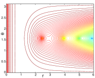
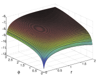
                    (a)                               (b)

Figure 2: (Color online) Magnitude of the two-anyon kernel versus the radius $r$ and the angle $\theta$ and $\phi$ for the configurations shown in Figs. 1 (a) and (b) respectively, for $m=3$. Fig. 2 (a) shows the first four zeros of the kernel lying on the line $\theta=\pi/2$, while Fig. 2 (b) shows that the kernel vanishes as either $r$ or $\phi$ approaches zero.

Eq. (39) can be generalized to the case of filling fractions different from $1/m$ where there are incompressible fractional quantum Hall states. In general, the ratio of the quasi-particle charge $e^{*}$ to the electron charge $e$ and the fractional statistics parameter $\alpha$ need not be equal to each other as they are for the Laughlin states. The two-particle kernel in the general case is given by

$$K_{2}({\vec{r}}_{1f},{\vec{r}}_{2f};{\vec{r}}_{1i},{\vec{r}}_{2i})$$

$$=\left(\frac{e^{*}}{2\pi el^{2}}\right)^{2}\exp[-\frac{e^{*}}{4e}(|z_{1f}|^{2}+|z_{2f}|^{2}+|z_{1i}|^{2}+|z_{2i}|^{2})$$

$$~{}~{}~{}~{}~{}~{}~{}~{}~{}~{}~{}~{}~{}~{}~{}~{}~{}~{}~{}~{}~{}~{}+\frac{e^{*}}{4e}(z_{1f}+z_{2f})(z_{1i}^{*}+z_{2i}^{*})]$$

$$\times~{}\sum_{p=0}^{\infty}~{}\frac{[(z_{1f}-z_{2f})(z_{1i}^{*}-z_{2i}^{*})/4m]^{2p+\alpha}}{\Gamma(2p+\alpha+1)}.$$ (40)

One can then show, using arguments similar to the ones which led from Eq. (30) to (39), that the two-particle kernel will have zeros when the rectangle in Fig. 1 (a) is a square with an area given by

$$2r^{2}~{}=~{}\frac{2\pi\hbar c}{eB}~{}\frac{e}{e^{*}}~{}(n~{}-~{}\frac{1}{2}~{}+~{}\frac{\alpha}{2}).$$ (41)

An example of the general case presented in Eq. (40) is provided by quasi-particles of the Jain states; these states appear at filling fractions of the form $\nu=p/(2np\pm 1)$, where $p$ and $n$ are integers. jain1 For $p>1$, the ratio $e^{*}/e$ is not equal to $\alpha$, unlike the special case of the Laughlin states which correspond to $p=1$. For $\nu=p/(2np+1)$, the fractional charge of the Jain state quasi-particles is given by $e^{*}=e/(2np+1)$. In one formulation, the statistical parameter has the form $\alpha=1-2n/(2np+1)$; this renders the $p>1$ Jain states more fermion-like in that $\alpha>1/2$, in comparison with the Laughlin states which have $\alpha<1/2$. fradkin

However, it is likely that a description of the quasi-particles for the Jain states will require us to beyond the LLL. One way to see this is to consider the composite fermion theory for fractional quantum Hall states. jain1 For instance, the state with $\nu=p/(2np+1)$ corresponds to composite fermions filling $p$ Landau levels. We will therefore discuss in Sec. III. D how the effects of higher Landau levels may be computed.

III.3 Experimental Realization

Based on the above analysis, we propose an experiment for measuring the charge and statistics of the quasi-particles. Consider a configuration in which there are two sources and two detectors of anyons, corresponding to the positions $z_{1i},z_{2i}$ and $z_{1f},z_{2f}$ respectively, which are arranged as a square as shown in Fig. 1. a ($\theta=\pi/2$). The sources and detectors can be created by bringing four edge states close together via a gate potential and setting the edges identified as the sources at a higher potential than those identified as the detectors, thus generalizing the principles used for observing the propagation of a single quasi-particle using a single source and a single detector. picciotto ; saminadayar Holding the area of the configuration and the filling fraction in the bulk fixed, one can gradually change the magnetic field and determine some successive values of the field where a simultaneous observation of the anyon tunneling current in the two detectors gives a null result. According to Eq. (41), a plot of the magnetic field $B$ versus the number of the zero $n$ will be a straight line whose slope is proportional to the charge $e^{*}$ and whose intercept gives the value of $(\alpha-1)/2$. Even if one mis-identifies the values of $n$ by a constant integer, the intercept will correctly give the fractional part of $(\alpha-1)/2$; this will be sufficient to identify the value of $\alpha$ in the range $[-1,1]$.

Experimentally, there may be a small uncertainty in the precise locations of the sources and detectors; further, the edge confining potential may be somewhat soft, with a width of the order of several magnetic lengths. Both of these would lead to an uncertainty in the area $2r^{2}$ in Eq. (41). This would lead to some uncertainty in the value of $e^{*}$ obtained from the slope of the straight line, but there would still be no uncertainty in the value of $\alpha$ obtained from the intercept. We therefore expect a determination of the statistics parameter via this method to be more robust than the charge.

In the discussion above, we have proposed holding the area of a certain configuration and the filling fraction in the bulk fixed, and finding some successive values of the magnetic field where the two-particle kernel vanishes. This is a reasonable procedure because as long as we are at a quantum Hall plateau, varying the magnetic field within some range does not change the filling fraction. However, this argument does require the region within the area of interest to be sufficiently clean and free of pinning impurities, so that no additional anyons appear or disappear there as the magnetic field is being varied. If additional anyons get trapped in that region, they would contribute to the two-particle kernel and destroy the simple relation between the magnetic field and the zeros of the kernel. Furthermore, our arguments do not take into account the invasive nature of the gates and the effects of the quantum Hall boundary. While we consider the effect of a boundary in the next section, a full-fledged treatment of the geometry proposed here is beyond the scope of the paper. However, we expect that with all considerations taken into account, the system will still exhibit effects of fractional charge and fractional statistics in coincidence measurements.

It has been argued that fractional statistics is a valid concept only if the distance between two quasi-particles is greater than about $10$ times the Landau length $l$. jain1 In typical experiments involving tunneling between quantum Hall edges, the tunneling distance is about $300~{}nm$. picciotto ; saminadayar This is much larger than $l$ which is of the order of $10~{}nm$ for a filling fraction of $1/3$. [That the tunneling amplitude is not negligible even though the ratio of the tunneling distance to the magnetic length is about 30 is probably due to the softness of the edge confining potential which gives it a width of several magnetic lengths. The implication of this softness for the determination of the charge and statistics parameter has been discussed above.] In terms of the configuration in Fig. 1 (a), we have $r/l\sim 30$. While such a large ratio certainly justifies the use of fractional statistics, it gives the value of the integer $n$ in Eq. (41) to be about $10^{3}$; it would be difficult to distinguish a fraction from such large values of $n$. To reduce the value of $n$ as far as possible and at the same time ensure that the idea of fractional statistics remains valid, we require values of $r/l$ which are not much larger than 10.

III.4 Higher Landau levels

There are several instances where a projection to the LLL will not suffice and higher Landau levels need to be invoked. Examples include finite temperature, length scales shorter than the magnetic length and time scales faster than the inverse cyclotron frequency, quasi-particles in non-Laughlin states such as most of the Jain states, and tunneling of quasi-particles in certain situations. Moreover, it is only by including higher Landau levels that one can consider dynamics; as we saw earlier, the kernel in the LLL has a trivial dependence on time. In what follows, as a start, we will calculate the effect of higher Landau levels on the two-anyon kernel using an imaginary time formalism. As before, we will ignore all interactions between the two particles apart from the exchange statistics. [An imaginary time formalism is directly relevant to a calculation of the density matrix at finite temperature; the imaginary time $\tau$ is inversely related to the temperature as $\tau=\hbar/(k_{B}T)$].

If the contribution of all Landau levels is taken into account, we expect the kernel to depend on the time coordinate. However, for the special cases of fermions and bosons, it turns out that the locations of the zeros of the kernel are independent of time and remain exactly at the same points where they were in the LLL calculation. This can be seen by substituting the expression in Eq. (7) in Eq. (17); we then find that the condition for the vanishing of the two-particle kernel is given by Eqs. (18-19) precisely as in the LLL.

We have not been able to find an analytic expression for the two-particle kernel for anyons in an arbitrary magnetic field analogous to the LLL expression given in Eq. (30). However, we can make some general statements about the wave functions and energy levels myrheim , and then about the zeros of the kernel in a particular limit of the imaginary time $\tau$. The two-particle kernel can again be factorized into a product of centre of mass and relative coordinate kernels as shown in Eq. (25). The centre of mass kernel is given by the expression in Eq. (7), with the charge, cyclotron frequency and coordinates in that equation being replaced by the appropriate centre of mass quantities; it is clear that this kernel does not have any zeros. Only the relative coordinate kernel is sensitive to the statistics parameter, and only this kernel can possibly have zeros. We will therefore consider only the relative coordinate kernel henceforth. Absorbing the appropriate Landau length in the complex coordinate $z=z_{1}-z_{2}$, and assuming as in Eq. (13) that the relative coordinate wave functions are of the form $\psi=f(z,z^{*})\exp(-|z|^{2}/4)$, we obtain the eigenvalue equation ${\tilde{H}}f=Ef$, where

$${\tilde{H}}~{}=~{}\hbar\Omega_{c}~{}[-~{}2\frac{\partial}{\partial z}\frac{\partial}{\partial z^{*}}~{}+~{}z^{*}\frac{\partial}{\partial z^{*}}],$$ (42)

where $\Omega_{c}$ is the cyclotron frequency for the relative coordinate system (it is determined by the charge $e^{*}$ and the reduced mass), and we have shifted the ground state energy to zero. Let us assume that the statistics parameter $\alpha$ lies in the range $0\leq\alpha\leq 1$. We then find that there are two types of eigenfunctions of Eq. (42):

(i) $f_{n,N}=z^{2n+\alpha}$ multiplied by a polynomial of degree $N$ in $zz^{*}$, where $n=0,1,2,\cdots$, and

(ii) $f_{-n,N}=z^{*2n-\alpha}$ multiplied by a finite polynomial of degree $N$ in $zz^{*}$, where $n=1,2,\cdots$.

The allowed values of $n$ are determined by the requirement that the wave function should not diverge as $z\to 0$. The form of the Hamiltonian in Eq. (42) implies that the eigenfunctions of types (i) and (ii) have energies $N\hbar\Omega_{c}$ and $(N+2n-\alpha)\hbar\Omega_{c}$ respectively. The LLL wave functions are a special case of the type (i) states, with $N=0$. [Note that for $\alpha=0(1)$, the wave functions given in (i) and (ii) are even (odd) under $z\to-z$, as expected from the symmetry (antisymmetry) of bosonic (fermionic) wave functions under an exchange of two particles. It is also interesting to observe that the energy levels of types (i) and (ii) do not coincide with each other if $\alpha$ is not equal to 0 or 1].

We can get an idea of the effect of higher Landau levels on the two-particle kernel as follows. For $0\leq\alpha\leq 1$, the lowest two sets of excited states are given by type (i) states with any $n$ but $N=1$ (these have $E=\hbar\Omega_{c}$), and the type (ii) state with $n=1$ and $N=0$ (this has $E=(2-\alpha)\hbar\Omega_{c}$). Let us define $\xi=e^{-\Omega_{c}\tau}$ and assume that this is small. We will ignore contributions from states with energies $E\geq 2\hbar\Omega_{c}$; hence we will keep terms only up to $\xi$ and $\xi^{2-\alpha}$, and ignore terms of order $\xi^{2}$ and higher. Our results will therefore be applicable for a time separation $\tau$ long compared to the inverse cyclotron frequency. To this order, the contribution to the kernel comes from the following normalized wave functions:

$$\psi_{n,0}({\vec{r}}) = \frac{1}{\sqrt{2\pi\Gamma(2n+\alpha+1)}}\left(\frac{z}{\sqrt{2}}\right)^{2n+\alpha}e^{-|z|^{2}/4},$$

$$\psi_{n,1}({\vec{r}}) = \sqrt{\frac{2n+\alpha+1}{2\pi\Gamma(2n+\alpha+1)}}\left(\frac{z}{\sqrt{2}}\right)^{2n+\alpha}$$

$$\times~{}\left(1~{}-~{}\frac{zz^{*}}{2(2n+\alpha+1)}\right)e^{-|z|^{2}/4},$$

$$\psi_{-1,0}({\vec{r}}) = \frac{1}{\sqrt{2\pi\Gamma(3-\alpha)}}\left(\frac{z^{*}}{\sqrt{2}}\right)^{2-\alpha}e^{-|z|^{2}/4}.$$ (43)

[The definition of $z$ in Eq. (43) differs by a numerical factor from the definition used in Eq. (29)]. The contribution to the two-particle kernel from the above states is given by

$$K_{2}({\vec{r}}_{1f},{\vec{r}}_{2f};{\vec{r}}_{1i},{\vec{r}}_{2i};\tau)$$ (44)

$$= \sum_{n=0}^{\infty}~{}\psi_{n,0}({\vec{r}}_{1f}-{\vec{r}}_{2f})~{}\psi_{n,0}^{*}({\vec{r}}_{1i}-{\vec{r}}_{2i})$$

$$~{}+ \sum_{n=0}^{\infty}~{}\psi_{n,1}({\vec{r}}_{1f}-{\vec{r}}_{2f})~{}\psi_{n,1}^{*}({\vec{r}}_{1i}-{\vec{r}}_{2i})~{}\xi$$

$$~{}+ \psi_{-1,0}({\vec{r}}_{1f}-{\vec{r}}_{2f})~{}\psi_{-1,0}^{*}({\vec{r}}_{1i}-{\vec{r}}_{2i})~{}\xi^{2-\alpha}.$$

Let us now introduce the variables $x=(z_{1f}-z_{2f})(z_{1i}^{*}-z_{2i}^{*})/2$, $x_{i}=|z_{1i}-z_{2i}|^{2}/2$ and $x_{f}=|z_{1f}-z_{2f}|^{2}/2$; note that $x_{i}x_{f}=|x|^{2}$. Eq. (44) can then be written in terms of confluent hypergeometric functions abramowitz as

$$K_{2} = \frac{x^{\alpha}~{}e^{-(x_{i}+x_{f})/2}}{2\pi\Gamma(\alpha+1)}~{}[~{}\{1~{}+~{}(1-x_{i}-x_{f})~{}\xi\}$$ (45)

$$\times~{}\frac{1}{2}\{M(1,1+\alpha,x)+M(1,1+\alpha,-x)\}$$

$$+~{}(x~{}+~{}x^{*})~{}\xi$$

$$\times~{}\frac{1}{2}\{M(1,1+\alpha,x)-M(1,1+\alpha,-x)\}$$

$$+~{}\alpha~{}\xi]~{}+~{}\frac{x^{*2-\alpha}~{}e^{-(x_{i}+x_{f})/2}}{2\pi\Gamma(3-\alpha)}~{}\xi^{2-\alpha}.$$

Let us now find where the zeros of the expression in Eq. (45) are. Since we know that the zeros of the kernel for bosons and fermions continue to satisfy the perpendicularity condition in Eq. (18), let us assume that this remains true for anyons in general and see if this gives us the locations of the zeros. This condition implies that $x$ is imaginary in Eq. (45); let us set $x=iy$, where $y>0$. Upon ignoring terms of order $\xi^{2}$ and higher, we find that the zeros of (45) are given by the relation

$$Re~{}M(1,1+\alpha,iy)~{}=~{}-\alpha~{}\xi~{}+~{}\frac{\Gamma(\alpha+1)}{\Gamma(3-\alpha)}~{}y^{2-2\alpha}~{}\xi^{2-\alpha},$$ (46)

where $Re$ denotes the real part. [Note that the condition for the zeros of the LLL kernel is recovered when one takes the limit $\tau\to\infty$, i.e., sets $\xi=0$ in Eq. (46)]. For $\alpha=0$, $Re~{}M(1,1+\alpha,iy)=\cos y$, and we find that Eq. (46) is satisfied if $y=(n-1/2)\pi$, where $n=1,2,3,\cdots$ (we ignore the last term in (46) which is of order $\xi^{2}$); this is the expected result for bosons as given by Eq. (36). For $\alpha=1$, $Re~{}M(1,1+\alpha,iy)=\sin y/y$, and Eq. (46) is satisfied if $y=n\pi$, where $n=1,2,3,\cdots$; this is the correct result for fermions as given by Eq. (36).

For $0<\alpha<1$, we find that Eq. (46) is satisfied for a discrete set of values of $y$, but these values depend on $\xi=e^{-\Omega_{c}\tau}$ and therefore on the time $\tau$. Using the asymptotic expression given in Eq. (34) for $y\to\infty$, we find that Eq. (46) takes the form

$$\cos~{}(y-\frac{\alpha\pi}{2})~{}=~{}-\alpha y^{\alpha}~{}\xi~{}+~{}\frac{\Gamma(\alpha+1)}{\Gamma(3-\alpha)}~{}y^{2-\alpha}~{}\xi^{2-\alpha}.$$ (47)

If $\xi$ is very small, the above equation can be used to find the correction from the zeros of the LLL kernel which lie at $y_{n}=(n-1/2+\alpha/2)\pi$; the correction can be seen to go to zero exponentially as $\tau\to\infty$. Eq. (47) shows that the zeros of the kernel will deviate appreciably from their locations in the LLL if either $\tau$ becomes comparable to the inverse cyclotron frequency, $\Omega_{c}\tau\sim 1$, or if a distance scale like the radius of the circle in Fig. 1 becomes much larger than the magnetic length, $y\gg 1$. This gives an idea of the correlation length and time scales in this problem; a discussion of the length and time scales in two-particle problems appearing in other areas of physics is given in Ref. baym, .

Although the above calculation was based only on the lowest few Landau levels, we conclude that in general, the locations of the zeros of the two-anyon kernel in an arbitrary magnetic field depend on the time. Thus the simple geometrical understanding of the zeros of the LLL kernel (based on the phase difference between two paths) given in Sec. III.2 needs to be modified when one considers the effect of higher Landau levels.

While the above treatment using imaginary time may be a valid starting point for studying finite temperature and tunneling, other processes would require using real time. Examples may include the propagation of Jain state quasi-particles; however, an explicit effective wave function description such as the one we have used here for Laughlin states is still lacking for the Jain states.

IV Tunneling across a quantum Hall strip

In this section, we return to the one-particle kernel and show how it can be used in a familiar setting, namely, to study tunneling between the edges of a quantum Hall strip. This will provide us with a microscopic understanding of some of the statements which have been made in the literature, in particular, the possibility of interference between tunneling due to multiple impurities. chamon1 We believe that the approach taken here is a first step towards connecting the bulk physics of the LLL to a boundary. A full understanding of bulk-mediated fractional statistics properties will require an analysis similar to the one presented here for two-particle properties and is beyond the scope of this paper.

We begin by examining a system of non-interacting electrons with filling fraction $\nu=1$. We consider a Hall strip which is infinitely extended along the $\hat{x}$-direction, and is confined in the $\hat{y}$-direction by a potential $eV(y)$, as shown in Fig. 3. For concreteness, we may take $V(y)$ to be simple harmonic. horsdal We choose the Landau gauge for the vector potential, so that the Hamiltonian is

$$H~{}=~{}\frac{1}{2\mu}~{}(p_{x}+\frac{eB}{c}y)^{2}~{}+~{}\frac{p_{y}^{2}}{2\mu}~{}+~{}eV(y).$$ (48)

The eigenstates of this Hamiltonian take the form

$$\psi_{k,n}(x,y)~{}=~{}e^{ikx}~{}f_{k,n}(y),$$ (49)

where $f_{k,n}$ satisfies the eigenvalue equation

$$[\frac{p_{y}^{2}}{2\mu}~{}+~{}\frac{1}{2\mu}~{}(\hbar k+\frac{eB}{c}y)^{2}~{}+~{}eV(y)]~{}f_{k,n}~{}=~{}E_{k,n}~{}f_{k,n}.$$ (50)

The wave number $k$ is quantized in units of $2\pi/L_{x}$ if the system has a length $L_{x}$; $k$ becomes a continuous variable as $L_{x}\to\infty$. If we work at zero temperature and the Fermi energy of the electrons is $E_{F}$, only those states will be occupied for which $E_{k,n}<E_{F}$. Let us assume that the confining potential is sufficiently weak (i.e., it is much less than the Landau level spacing $\hbar\omega_{c}$ in the region of interest), so that only states with $n=0$ can be filled. As a function of $k$, the filled states lie within some interval $k_{1}<k<k_{2}$. Assuming that $V(y)$ is an even function of $y$, we have $k_{2}=k_{F}$ and $k_{1}=-k_{F}$, and the corresponding wave functions are centered about $y=-y_{F}$ and $y_{F}$ respectively, where

$$y_{F}~{}=~{}k_{F}l^{2},$$ (51)

$l$ being the Landau length. (It is a well-known feature of states in the Landau gauge that the momentum in the $\hat{x}$-direction and the position in the $\hat{y}$-direction are correlated with each other). In the presence of the confining potential, the energy levels in the LLL are no longer degenerate. If the confining potential $eV(y)$ is weak, there is an effective electric field at the edge given by ${\cal E}=-(dV/dy)_{y=y_{F}}$. Then the electrons have a drift velocity given by $v_{F}=c|{\cal E}/B|$. If $|{\cal E}/B|\ll 1$, we can show that $v_{F}=(1/\hbar)(\partial E_{k,0}/\partial k)_{k=k_{F}}$. girvin The electrons have a negative velocity $-v_{F}$ at the upper edge at $y=y_{F}$, and a positive velocity $v_{F}$ at the lower edge at $y=-y_{F}$.

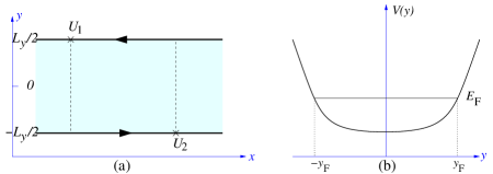
Figure 3: (Color online) Quantum Hall state in a strip geometry of length $L_{x}$ and width $L_{y}$ in the presence of a confining potential $V(y)$. The states are filled up to a Fermi energy $E_{F}$, corresponding to a strip width of $2y_{F}=L_{y}$. Tunneling across the strip can take place via impurities denoted by $U_{i}$.

In order to have tunneling between the two edges, it is necessary to break the translation invariance in the $\hat{x}$-direction. As a simple model for this, let us introduce an impurity potential of the form $U_{1}(x,y)=U_{1}\delta(x-x_{1})\delta(y-y_{1})$; we have introduced the subscript 1 because we will later consider the effect of more than one impurity. Assuming that $U_{1}$ is small, we will use the Born approximation to compute the tunneling amplitude produced by this impurity. Although the impurity potential has non-zero matrix elements between states with all possible energies, we will see that in the asymptotic regions $x\to\pm\infty$, the impurity causes scattering only between pairs of states with the same energy. We consider an electron coming in from the left in the state $\psi_{k_{F},0}$ with energy $E_{F}$. Under the lowest order Born approximation, we have

$$\psi({\vec{r}}) = \psi_{k_{F},0}({\vec{r}})$$

$$-~{}\int d^{2}{\vec{r}}~{}^{\prime}~{}G({\vec{r}},{\vec{r}}~{}^{\prime},E_{F})~{}U_{1}({\vec{r}}~{}^{\prime})~{}\psi_{k_{F},0}({\vec{r}}~{}^{\prime}),$$

where the retarded Green’s function is given by

$$G({\vec{r}},{\vec{r}}~{}^{\prime},E)~{}=~{}\sum_{n}~{}\int~{}\frac{dk}{2\pi}~{}\frac{\psi_{k,n}({\vec{r}})~{}\psi_{k,n}^{*}({\vec{r}}~{}^{\prime})}{E_{k,n}~{}-~{}E~{}-~{}i\epsilon}.$$ (53)

We recall that the Fourier transform of the above Green’s function, $G({\vec{r}},{\vec{r}}~{}^{\prime},t)$, vanishes for $t<0$ and is equal to $i/\hbar$ times the one-particle kernel for $t>0$.

We now evaluate Eq. (LABEL:born) using some approximations. First, we will only consider contributions to the Green’s function coming from states with $n=0$ whose energies lie in the vicinity of $E_{F}$. For these states, we make the linearized approximation

$$E_{k,0} = E_{F}~{}+~{}\hbar v_{F}(k-k_{F})~{}~{}{\rm near}~{}~{}k=k_{F},$$ (54)

$$= E_{F}~{}-~{}\hbar v_{F}(k+k_{F})~{}~{}{\rm near}~{}~{}k=-k_{F},$$

and we then extend the range of the integration variable $k$ up to $\pm\infty$. Secondly, since the confining potential $eV(y)$ is weak, we approximate the wave functions by

$$\psi_{k,0}({\vec{r}})~{}=~{}e^{ikx}\left(\frac{1}{\pi l^{2}}\right)^{1/4}\exp[-~{}(y\pm y_{F})^{2}/(2l^{2})]$$

(55)

for $k$ close to $\pm k_{F}$ respectively. Eq. (LABEL:born) then gives

$$\psi({\vec{r}}) = \psi_{k_{F},0}~{}+~{}r_{L}~{}\psi_{-k_{F},0}~{}~{}{\rm for}~{}~{}x\to-~{}\infty,$$ (56)

$$= t_{L}~{}\psi_{k_{F},0}~{}~{}{\rm for}~{}~{}x\to\infty,$$

where the reflection and transmission amplitudes are given by

$$r_{L} = -~{}\frac{iU_{1}}{\hbar v_{F}}~{}e^{i2k_{F}x_{1}}$$

$$~{}\times~{}\left(\frac{1}{\pi l^{2}}\right)^{1/2}\exp[-~{}(y_{1}^{2}+y_{F}^{2})/l^{2}],$$

$$t_{L} = 1~{}-~{}\frac{iU_{1}}{\hbar v_{F}}\left(\frac{1}{\pi l^{2}}\right)^{1/2}\exp[-~{}(y_{1}+y_{F})^{2}/l^{2}]$$

to first order in $U_{1}$. The Gaussian factor appearing in $r_{L}$ is dependent on $(y_{1}+y_{F})^{2}+(y_{1}-y_{F})^{2}$, i.e., the sum of the squares of the distances of the impurity from the two edges. The probability of tunneling between the two edges is given by $|r_{L}|^{2}$. Similarly, for an electron coming in from the right in the state $\psi_{-k_{F},0}$ with energy $E_{F}$, Eq. (LABEL:born) gives

$$\psi({\vec{r}}) = \psi_{-k_{F},0}~{}+~{}r_{R}~{}\psi_{k_{F},0}~{}~{}{\rm for}~{}~{}x\to\infty,$$ (58)

$$= t_{R}~{}\psi_{-k_{F},0}~{}~{}{\rm for}~{}~{}x\to-~{}\infty,$$

where

$$r_{R} = -~{}\frac{iU_{1}}{\hbar v_{F}}~{}e^{-i2k_{F}x_{1}}$$

$$~{}\times~{}\left(\frac{1}{\pi l^{2}}\right)^{1/2}\exp[-~{}(y_{1}^{2}+y_{F}^{2})/l^{2}],$$

$$t_{R} = 1~{}-~{}\frac{iU_{1}}{\hbar v_{F}}\left(\frac{1}{\pi l^{2}}\right)^{1/2}\exp[-~{}(y_{1}-y_{F})^{2}/l^{2}].$$

We can introduce a $2\times 2$ scattering matrix which relates the outgoing states to the incoming states,

$$S = \left(\begin{array}[]{cc}r_{L}&t_{R}\\ t_{L}&r_{R}\end{array}\right).$$ (62)

We find, as required, that $S$ is unitary to first order in $U_{1}$.

We can now consider the effects of several impurities which produce a potential of the form

$$U(x,y)~{}=~{}\sum_{n}~{}U_{n}~{}\delta(x-x_{n})~{}\delta(y-y_{n}).$$ (63)

To first order in the $U_{n}$, we get

$$r_{L} = -~{}\frac{i}{\hbar v_{F}}~{}\sum_{n}~{}U_{n}~{}e^{i2k_{F}x_{n}}~{}\exp[-~{}y_{n}^{2}/l^{2}]$$ (64)

$$~{}\times~{}\left(\frac{1}{\pi l^{2}}\right)^{1/2}\exp[-~{}y_{F}^{2}/l^{2}],$$

and $r_{R}=-~{}r_{L}^{*}$. We see that there are certain configurations of two or more impurities which give zero reflection. We can understand this using an Aharonov-Bohm phase argument in a simple case involving two weak barriers, chamon1 as shown in Fig. 3. Consider two impurities with equal strengths $U_{1}=U_{2}$, and $y_{1}=\pm y_{2}$. According to Eq. (64), $r_{L}$ vanishes if

$$2k_{F}(x_{2}-x_{1})~{}=~{}\frac{2y_{F}(x_{2}-x_{1})}{l^{2}}~{}=~{}(2n+1)~{}\pi.$$ (65)

Now, $2y_{F}(x_{2}-x_{1})$ is the area of the rectangle bounded by the two edges and by the lines $x=x_{1}$ and $x=x_{2}$. If we imagine that the tunneling between the edges occurs along the straight lines $x=x_{1}$ and $x=x_{2}$, Eq. (65) represents the Aharonov-Bohm phase enclosed by the edges and the tunneling paths. The reflection amplitude vanishes if this phase is an odd multiple of $\pi$.

Although the results obtained so far are for the case of electrons with $\nu=1$, we expect that certain aspects of the results will continue to remain valid for quasi-particles with charge $\pm e/m$. The effective width of the Hall strip, $2y_{F}$, is expected to be the same for electrons and for quasi-particles. The forms of the wave function in Eq. (55) and therefore of the tunneling amplitude in Eq. (64) are also expected to remain the same for quasi-particles, except that the factors of $y^{2}/l^{2}$ in the exponentials will change to $y^{2}/(ml^{2})$ due to the charge of the quasi-particles. Finally, the condition for the vanishing of the reflection amplitude due to two impurities given in Eq. (65) will change to $2y_{F}(x_{2}-x_{1})/(ml^{2})=(2n+1)\pi$; this is again because the quasi-particle charge is different from that of electrons, but the area of the rectangle continues to be $2y_{F}(x_{2}-x_{1})$.

Since the exponentials appearing in the tunneling amplitudes $r_{L}$ and $r_{R}$ depend on the charge of the tunneling particle, the tunneling amplitude will be much larger for quasi-particles with charge $\pm e/m$ than for electrons with charge $e$. auerbach The situation is of course complicated by the fact that the effective tunneling amplitude is governed by a renormalization group equation and therefore depends on the energy scale of interest. wen1 ; wen2 ; wen3 ; kane2 What we have calculated in this section is the bare tunneling amplitude.

We have considered above the tunneling of a single particle, called $A$, from one edge to another without taking into account its interaction with any other particles. One can consider a case in which a second particle, called $B$, is pinned to some fixed point inside the strip; let us denote the location of this particle by $(x_{B},y_{B})$. If the two particles are, say, quasi-holes, the expression given in Eq. (64) for the tunneling due to several impurities will need to be modified in order to take their fractional statistics into account. For the reflection amplitude $r_{L}$ in (64), the contribution from an impurity which lies to the left of particle $B$ (i.e., $x_{n}<x_{B}$) would remain unchanged, while the contribution from an impurity which lies to the right of $B$ ($i.e.,x_{n}>x_{B}$) would carry an extra phase of $e^{-i2\pi\alpha}$. This is because the tunneling path corresponding to the second impurity has an extra phase compared to the tunneling path corresponding to the first impurity; this is given by the phase of one anyon going around another in the clockwise direction.

The arguments given above explain why the total tunneling amplitude for one particle will oscillate if one varies either the magnetic field or the number of other particles lying within the rectangle formed by two impurities. This provides a microscopic justification for some of the statements made in Ref. chamon1, .

The calculations in this section can be generalized to the case of quantum Hall systems in which more than two edges come close to each other in certain regions safi ; vishveshwara1 ; kim ; grosfeld ; oshikawa ; das ; comforti . We expect that the statement made after Eq. (LABEL:rl), namely, that an impurity-induced tunneling amplitude between two edges depends on the sum of the squares of the distances of the impurity from the two edges, will remain valid in general.

V Correlations along edges of a quantum Hall system

In this section, we discuss the two-point correlators along the edges of a quantum Hall system. We will consider two possible geometries, namely, a long strip and a circular droplet. Since our main aim is to show the effects of different geometries, we restrict our attention to the case of non-interacting electrons with $\nu=1$ for simplicity.

Let us first consider the strip geometry. We assume a confining potential as in Sec. IV; hence the states in the LLL are labeled only by the wave number $k$ in the $\hat{x}$-direction. The ground state $|G\rangle$ of the electrons is taken to be one in which all states are filled up to a Fermi energy $E_{F}$ which corresponds to $k=\pm k_{F}$. For simplicity, we ignore the effect of the confinement when writing down the wave functions,

$$\psi_{k,0}({\vec{r}})~{}=~{}e^{ikx}\left(\frac{1}{\pi l^{2}}\right)^{1/4}\exp[-~{}(y+kl^{2})^{2}/(2l^{2})].$$

We will compute the correlator

$$C({\vec{r}}_{1};{\vec{r}}_{2};t)~{}=~{}\langle G|\Psi^{\dagger}({\vec{r}}_{1},0)\Psi({\vec{r}}_{2},t)|G\rangle,$$ (67)

where the second quantized field $\Psi$ is given by

$$\Psi({\vec{r}},t)~{}=~{}\sum_{n}~{}\int~{}\frac{dk}{2\pi}~{}c_{k,n}~{}\psi_{k,n}({\vec{r}})e^{-iE_{k,n}t/\hbar},$$ (68)

and $~{}\{c_{k,n},c_{k^{\prime},n^{\prime}}^{\dagger}\}=2\pi\delta(k-k^{\prime})\delta_{n,n^{\prime}}$. For ${\vec{r}}_{1}=(0,y_{1})$ and ${\vec{r}}_{2}=(x,y_{2})$, we obtain the expression for the equal-time correlator

$$C(0,y_{1};x,y_{2};0) = \int_{-k_{F}}^{k_{F}}~{}\frac{dk}{2\pi}~{}e^{ikx}~{}\left(\frac{1}{\pi l^{2}}\right)^{1/2}$$

$$~{}~{}~{}\times~{}\exp[-~{}(y_{1}+kl^{2})^{2}/(2l^{2})]$$

$$~{}~{}~{}\times~{}\exp[-~{}(y_{2}+kl^{2})^{2}/(2l^{2})].$$

It is convenient to define the dimensionless variables $X=x/l$ and $Y_{F}=k_{F}l$. We now consider the following cases.

(i) The two points are on the same edge, say the lower edge $y_{1}=y_{2}=-y_{F}$, where $y_{F}$ is related to $k_{F}$ through Eq. (51). After shifting and rescaling $k$ to be dimensionless, we get

$$C(0,-y_{F};x,-y_{F};0)~{}=~{}\frac{1}{2\pi^{3/2}l^{2}}~{}\int_{-2Y_{F}}^{0}dk~{}e^{-k^{2}+ikX}.$$ (70)

If the strip is much wider than the Landau length, namely, $Y_{F}\gg 1$, the integral in Eq. (70) is equal to $(1/2)e^{-X^{2}/4}[\sqrt{\pi}-iX{}_{1}F_{1}(1/2;3/2;X^{2}/4)]$. gradshteyn For $X^{2}/4\to\infty$, this goes to zero as $-i/X$. abramowitz The last result can be obtained in a different way. In the limit of large $|X|$, the integral only gets a contribution from small values of $k$. The asymptotic value of the integral therefore does not depend on how the integrand is cut off at large values of $|k|$. If we choose a cut-off such as $e^{\epsilon k}$, where we eventually take $\epsilon\to 0^{+}$, the integral can be done analytically and we get $-i/X$.

(ii) The two points are on opposite edges, $y_{1}=-y_{F}$ and $y_{2}=y_{F}$. After rescaling, we get

$$C(0,-y_{F};x,y_{F};0)~{}=~{}\frac{1}{2\pi^{3/2}l^{2}}~{}e^{-Y_{F}^{2}}~{}\int_{-Y_{F}}^{Y_{F}}~{}dk~{}e^{-k^{2}+ikX}.$$ (71)

If the strip is very wide, the limits of the integration can be replaced by $\pm\infty$, and we find that the correlator goes as $e^{-X^{2}/4}$. On the other hand, if the strip width is of the order of the Landau length, i.e., $Y_{F}\sim 1$, the magnitude of the correlator exhibits oscillations and, in fact, vanishes for a discrete set of values of $X$. For small values of $Y_{F}$, the wavelength of the oscillations is given by $\pi/Y_{F}$. Oscillations also occur, although they are less prominent, if the two points lie on the same edge and $Y_{F}\sim 1$. Fig. 4 shows these oscillations in the correlator (given in units of $1/(2\pi^{3/2}l^{2})$) for $Y_{F}=0.5$.

The results discussed above show that the usual discussions of edge states and bulk physics have to be modified in the case of highly confined geometries. This needs to be kept in mind when one is trying to understand the results of experiments performed under such conditions.

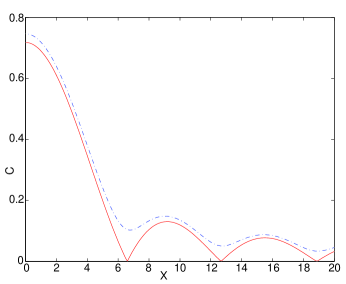
Figure 4: (Color online) Magnitude of the two-point correlator versus the separation $X$, for $Y_{F}=0.5$. The solid and dash-dot lines show the cases where the two points lie on opposite edges and on the same edge respectively.

Let us now consider a circular geometry with a confining potential $V(r)$ which we will not explicitly specify. We choose the symmetric gauge, and use the LLL wave functions given in Eq. (14). In the presence of the confining potential, we take the ground state to be one in which all states from $n=0$ to $N$ are filled, where we assume that $N\gg 1$. The radius of the system is given by $r_{F}=l\sqrt{2N}$. Let us take the two points ${\vec{r}}_{1},~{}{\vec{r}}_{2}$ to lie on the circumference, with ${\vec{r}}_{1}=r_{F}(1,0)$ and ${\vec{r}}_{2}=r_{F}(\cos\phi,\sin\phi)$. We define a dimensionless radius $R=r_{F}/l=\sqrt{2N}$. The equal-time correlator is then given by

$$C({\vec{r}}_{1};{\vec{r}}_{2};0)~{}=~{}\frac{1}{2\pi l^{2}}~{}\sum_{n=0}^{N}~{}\frac{1}{n!}~{}\left(\frac{R^{2}e^{i\phi}}{2}\right)^{n}~{}\exp[-\frac{1}{2}R^{2}].$$ (72)

For large values of $N$, we can evaluate the sum using saddle point methods. bender We first expand the terms in Eq. (72) around $n=N$ up to second order in $n-N$; this yields

$$C({\vec{r}}_{1};{\vec{r}}_{2};0)~{}\simeq~{}\frac{e^{iN\phi}}{2\pi^{3/2}l^{2}\sqrt{2N}}~{}\sum_{n=0}^{N}e^{i(n-N)\phi-(n-N)^{2}/2N}.$$ (73)

If $\phi\ll\pi$, we can replace the sum in Eq. (73) by an integral. Introducing the quantity $k=(n-N)/\sqrt{2N}$ which becomes a continuous variable as $N\to\infty$, we find that

$$C({\vec{r}}_{1};{\vec{r}}_{2};0)~{}\simeq~{}\frac{e^{iN\phi}}{2\pi^{3/2}l^{2}}~{}\int_{-\infty}^{0}~{}dk~{}e^{-k^{2}+ikR\phi}.$$ (74)

This has exactly the same form as in Eq. (70), up to a phase $e^{iN\phi}$, with $X$ being equal to the arc length $R\phi$. On the other hand, if $\phi\sim\pi$, we cannot replace the sum in Eq. (73) by an integral. However, the sum is then dominated by small values of $n-N$, and we can replace the Gaussian cut-off $e^{-(n-N)^{2}/2N}$ by $e^{\epsilon(n-N)}$, where we eventually take $\epsilon\to 0^{+}$. On summing up the series, we obtain jain1 ; wen3

$$C({\vec{r}}_{1};{\vec{r}}_{2};0)~{}\simeq~{}-~{}\frac{e^{iN\phi}}{2\pi^{3/2}l^{2}}~{}\frac{ie^{i\phi/2}}{2R\sin(\phi/2)}.$$ (75)

For $\phi\to 0$ but $R\phi\gg 1$, Eq. (75) agrees with the result one obtains from Eq. (74).

Finally, let us discuss the finite time behavior of the correlators for the cases when the two points lie on the same edge of a strip, or on the circumference of a circle. At large separations, i.e., $x\to\infty$ for the strip or $r_{F}\phi\to\infty$ for the circle, the contribution to the correlator mainly comes from states close to the Fermi energy. For such states, we can use the linearized approximation for the dispersion, $E_{k,0}=\hbar v_{F}(k-k_{F})$ near the lower edge of the strip, or $E_{n}=\hbar v_{F}(n-N)/r_{F}$ near the circumference of the circle; while writing these down, we have re-defined the Fermi energy so that it is zero at the edge. We then see that the finite-time correlator can be obtained from the equal-time correlator by replacing $x$ by $x-v_{F}t$ at the lower edge of the strip, or $r_{F}\phi$ by $r_{F}\phi-v_{F}t$ at the circumference of the circle.

The calculations in this section are valid when the filling fraction $\nu$ is equal to 1. For $\nu=1/m$, it is known that the two-point correlators for electrons and quasi-particles decay as non-trivial powers of the separation which can be found using the technique of bosonization wen3 ; stone ; gogolin ; rao ; giamarchi . However, bosonization only works at distances which are large compared to the Landau length. Hence, one may require other techniques to study short-distance properties for $\nu=1/m$.

VI Summary

In this paper, we have studied the one- and two-particle kernels of charged particles moving in a strong magnetic field. We have shown that the two-particle kernel in the bulk of a quantum Hall system contains information about two important properties of the particles. Namely, the kernel vanishes for a discrete set of geometries of the initial and final positions in a way which is determined by the exchange statistics; the kernel also vanishes as the particles approach each other with a power law which is related to a generalized exclusion statistics. These angular and distance dependences of the kernel should be observable in the correlations of two-particle tunnelings in appropriate gate-defined quantum Hall geometries. We have proposed an experiment which can use the vanishing of the kernel to determine the charge and fractional statistics of the particles. Our analysis is expected to work best for fractional quantum Hall states lying in the Laughlin sequence with the filling fraction being given by the inverse of an odd integer. For such states, a lowest Landau level treatment is adequate, and the charge and statistics parameter of quasi-particles are equal to each other.

The one-particle kernel can be used to study impurity-induced tunneling between different edges of a quantum Hall strip which contains some impurities. Here too we find that certain arrangements of the impurities give rise to a vanishing tunneling amplitude. Finally, we have studied the two-point correlator along different edges of a quantum Hall strip and droplet. We find that the correlator has a rich structure if the separation between the two points and the width of the strip are of the order of the Landau length.

To conclude, we see that geometry plays an important, and sometimes surprising, role in the propagation of particles through the bulk of a quantum Hall system. A complete understanding of experiments which measure one- and two-particle properties therefore requires us to take into account all the geometrical aspects of the problem.

Appendix A One-particle kernel in a magnetic field

To derive the kernel given in Eq. (6), we start with the action

$$S~{}=~{}\int_{0}^{t}~{}dt^{\prime}~{}[~{}\frac{\mu}{2}({\dot{x}}^{2}~{}+~{}{\dot{y}}^{2})~{}+~{}\frac{eB}{2c}(x{\dot{y}}~{}-~{}y{\dot{x}})~{}].$$ (76)

We find the Euler-Lagrange equations of motion arising from this action, and solve them using the boundary conditions ${\vec{r}}(t^{\prime}=0)={\vec{r}}_{i}$ and ${\vec{r}}(t^{\prime}=t)={\vec{r}}_{f}$. Substituting the solution in Eq. (76), we obtain the classical action

$$S_{cl}({\vec{r}}_{f};{\vec{r}}_{i};t) = \frac{\mu\omega_{c}\cot(\omega_{c}t/2)}{4}~{}({\vec{r}}_{f}-{\vec{r}}_{i})^{2}$$ (77)

$$+~{}\frac{\mu\omega_{c}}{2}~{}{\hat{z}}\cdot{\vec{r}}_{i}\times{\vec{r}}_{f}.$$

Since the action is quadratic in $x$ and $y$, a path integral argument shows that the kernel must be of the form feynman

$$K_{1}({\vec{r}}_{f};{\vec{r}}_{i};t)~{}=~{}f(t)~{}e^{iS_{cl}({\vec{r}}_{f};{\vec{r}}_{i};t)/\hbar},$$ (78)

where $f(t)$ is independent of ${\vec{r}}_{i}$ and ${\vec{r}}_{f}$. Next, we know that the kernel is given by the sum

$$K_{1}({\vec{r}}_{f};{\vec{r}}_{i};t)~{}=~{}\sum_{n}~{}\psi_{n}({\vec{r}}_{f})~{}\psi_{n}^{*}({\vec{r}}_{i})~{}e^{-iE_{n}t/\hbar},$$ (79)

and therefore satisfies the equation

$$[~{}i\hbar~{}\frac{\partial}{\partial t}~{}-~{}H_{f}~{}]~{}K_{1}({\vec{r}}_{f};{\vec{r}}_{i};t)~{}=~{}0,$$ (80)

where $H_{f}$ is the Hamiltonian in Eq. (5) written in terms of ${\vec{r}}_{f}$ and $\partial/\partial{\vec{r}}_{f}$. This leads to the following first order differential equation for the function $f(t)$ in Eq. (78),

$$\frac{df}{dt} = -~{}\frac{i}{\hbar}~{}\left[\frac{\partial S_{cl}}{\partial t}~{}+~{}e^{-iS_{cl}/\hbar}~{}H_{f}~{}e^{iS_{cl}/\hbar}\right]~{}f$$ (81)

$$= -~{}\frac{\omega_{c}}{2}~{}\cot(\frac{\omega_{c}t}{2})~{}f.$$

The solution of this equation is

$$f(t)~{}=~{}\frac{A}{\sin(\omega_{c}t/2)}.$$ (82)

Finally, the constant $A$ can be fixed by demanding that the kernel should reduce to the free particle result in Eq. (4) as $\omega_{c}\to 0$. This yields $A=\mu\omega_{c}/(i4\pi\hbar)$. Putting all this together gives Eq. (6).

Appendix B Alternative formalisms for a two-anyon system

Consider a system of two anyons with a relative coordinate ${\vec{r}}$ and mass $\mu/2$; let us assume that there are no external fields or potentials. One can proceed in two different ways using the polar coordinates $(r,\phi)$. wilczek2 ; forte ; lerda ; khare ; myrheim ; ouvry

In the first formalism, the Lagrangian and Hamiltonian are given by

$$L = \frac{\mu}{4}~{}({\dot{r}}^{2}~{}+~{}r^{2}{\dot{\phi}}^{2}),$$

$${\rm and}~{}~{}H = \frac{1}{\mu}~{}(p_{r}^{2}~{}+~{}\frac{p_{\phi}^{2}}{r^{2}}),$$ (83)

where $p_{\phi}=-i\hbar\partial/\partial\phi$. In this case, the wave functions are taken to be multi-valued with the property that $\psi(\phi+\pi)=e^{i\pi\alpha}\psi(\phi)$; this is satisfied if the angular dependence of the wave function is of the form $e^{i(2p+\alpha)\phi}$, where $p$ is an integer.

In the second formalism, the Lagrangian and Hamiltonian are given by

$$L = \frac{\mu}{4}~{}({\dot{r}}^{2}~{}+~{}r^{2}{\dot{\phi}}^{2})~{}-~{}\alpha{\dot{\phi}},$$

$${\rm and}~{}~{}H = \frac{1}{\mu}~{}\left(p_{r}^{2}~{}+~{}\frac{(p_{\phi}+\alpha)^{2}}{r^{2}}\right).$$ (84)

In this case, the wave functions are single-valued; the angular dependence is of the form $e^{i2p\phi}$, where $p$ is an integer. The energy levels are of course the same in the two formalisms.

Let us now consider studying the problem using path integrals. If we exchange the two particles in an anticlockwise sense, the coordinate $\phi$ changes by $\pi$. In the second formalism, the path integral picks up a phase of $e^{-i\pi\alpha}$ due to the last term in the Lagrangian in Eq. (84). For a clockwise exchange of the two particles, $\phi$ changes by $-\pi$ and the path integral picks up a phase of $e^{i\pi\alpha}$. We thus see that the exchange phases picked up by the wave function in the first formalism and by the path integral in the second formalism have opposite signs.

Appendix C Charge and statistics of quasi-holes in a fractional quantum Hall system

The charge and statistics of quasi-holes in a quantum Hall system with filling fraction equal to $1/m$, where $m$ is an odd integer, has been derived in Refs. laughlin2, ; halperin, ; arovas, . Briefly, the derivation is based on the Laughlin variational wave functions for the ground state $\psi_{0}$ with no quasi-holes, $\psi_{1}(\eta_{1})$ describing one quasi-hole located at $\eta_{1}$ (using complex notation), and $\psi_{1}(\eta_{1},\eta_{2})$ describing two quasi-holes located at $\eta_{1}$ and $\eta_{2}$. These are given by

$$\psi_{0} = \prod_{i<j}~{}(z_{i}~{}-~{}z_{j})^{m}~{}\exp[-\frac{1}{4}~{}\sum_{i}~{}|z_{i}|^{2}],$$

$$\psi_{1}(\eta_{1}) = \prod_{i}~{}(z_{i}~{}-~{}\eta_{1})~{}\psi_{0},$$

$$\psi_{2}(\eta_{1},\eta_{2}) = \prod_{i}~{}(z_{i}~{}-~{}\eta_{1})(z_{i}~{}-~{}\eta_{2})~{}\psi_{0},$$ (85)

where $z_{i}$ denote the locations of the electrons. We compute the phase picked up by the wave function $\psi_{1}(\eta_{1})$ when $\eta_{1}$ is taken around a large anticlockwise loop enclosing an area $A$. Equating that to the Aharonov-Bohm phase of a particle of charge $e^{*}$ moving in a magnetic field, one finds that the quasi-hole has charge $-e/m$. Then we consider the phase picked up by $\psi_{2}(\eta_{1},\eta_{2})$ when $\eta_{1}$ is taken around a large anticlockwise loop of area $A$ which encloses the quasi-hole at $\eta_{2}$. This phase is given by a sum of the Aharonov-Bohm phase due to the magnetic field and twice the exchange phase; the latter arises because taking one quasi-hole around another gives a phase which is twice the phase picked up when the two quasi-holes are exchanged. We thus discover that the exchange phase is $\pi/m$. Now, the wave function $\psi_{2}$ is clearly single-valued. Following the arguments given in Appendix B, we therefore identify $\alpha=-1/m$.

Next, let us consider the wave function of two quasi-holes in the LLL, where the quasi-holes are now to be thought of as two ‘elementary’ objects moving in a vacuum, not as collective excitations of many electrons as described by $\psi_{2}$ above. Since the sign of the quasi-hole is opposite to the sign of an electron, the wave function must be a function of $z^{*}$ times a Gaussian. The fact that $\alpha=-1/m$ now implies that if we use a multi-valued wave function, the dependence of the wave function on the relative coordinate must be of the form $(z_{1}^{*}-z_{2}^{*})^{2p+1/m}$, where $p$ is a non-negative integer.

Although the wave function of quasi-holes is a function of $z^{*}$ in the LLL (if the wave function of electrons is a function of $z$), we have taken the quasi-hole wave functions to be functions of $z$ and changed $\alpha\to 1/m$ in the main body of the paper in order to use the same notation everywhere.

Appendix D Quasi-hole exclusion statistics

We present here a state counting argument to show that quasi-holes in the LLL exhibit exclusion statistics haldane ; veigy ; johnson ; su . The polynomial part of a state of $N_{q}$ quasi-holes in a sea of $N_{e}$ electrons at filling fraction $1/m$ is given by

$$\psi(z_{1},\ldots,z_{N_{e}};\zeta_{1},\ldots,\zeta_{Nq})$$

$$~{}=~{}\prod_{i=1}^{N_{e}}~{}\prod_{a=1}^{N_{q}}~{}(z_{i}-\zeta_{a})~{}\prod_{i<j}~{}(z_{i}-z_{j})^{m}.$$ (86)

This is a polynomial, in any individual $z_{i}$, of maximum degree

$$N_{\phi}~{}=~{}m(N_{e}-1)+N_{q}~{}=~{}\frac{eB}{2\pi\hbar c}~{}(\hbox{Area}).$$ (87)

Note that we have to keep this area (and not $N_{e}$) fixed as we count the dimension of the quasi-hole Hilbert space. Now

$$\prod_{i=1}^{N_{e}}~{}(z_{i}-\zeta) = e_{N_{e}}~{}-~{}e_{N_{e}-1}\zeta~{}+~{}e_{N_{e}-2}\zeta^{2}~{}+~{}\cdots$$ (88)

$$+~{}(-1)^{N_{e}}\zeta^{N_{e}},$$

where $e_{n}(z_{i})$ denote the elementary symmetric functions in the $N_{e}$ variables $z_{i}$. They can be represented as single-column Young diagrams with at most $N_{e}$ boxes in the column.

A general linear combination of quasi-hole states is therefore a Laughlin factor multiplied by a linear combination of products of $N_{q}$ such elementary symmetric functions. The total number of such functions is given by the number of partitions that can be fitted into an $N_{e}$-by-$N_{q}$ rectangle. This number is the number of positive-going random walks on an integer lattice from $(0,0)$ to $(N_{e},N_{q})$. It is therefore the coefficient of $x^{N_{e}}y^{N_{m}}$ in the expansion of $(x+y)^{N_{e}+N_{m}},$ which is given by

$${{N_{e}+N_{q}}\choose{N_{q}}}~{}=~{}{{D+N_{q}-1}\choose{N_{q}}}.$$ (89)

In the second form, we have eliminated $N_{e}$ in favor of $N_{\phi}$ and defined

$$D_{q}~{}=~{}\frac{N_{\phi}}{m}~{}-~{}\frac{1}{m}(N_{q}-1)~{}+~{}[2-1/m],$$ (90)

where $[r]$ denotes the integer part of $r$. Ignoring the term $[2-1/m]$ which is thermodynamically insignificant, su we see that the expression for $D$ is of the Haldane form haldane

$$D~{}=~{}\frac{N_{\phi}}{m}~{}-~{}g(N_{q}-1),$$ (91)

with the exclusion parameter $g=1/m$. ($g$ is 1 for fermions and 0 for bosons). Note that $N_{\phi}/m$ is the number of single particle states available to a charge $e/m$ particle in a region threaded by $N_{\phi}$ electron flux units.

References

- (1)
- (2) J. Leinaas and J. Myrheim, Nuovo Cimento B 37, 1 (1977).
- (3) F. Wilczek, Phys. Rev. Lett. 48, 1144 (1982); 49, 957 (1982).
- (4) R. B. Laughlin, Phys. Rev. Lett. 50, 1395 (1983); Rev. Mod. Phys. 71, 863 (1999).
- (5) R. B. Laughlin, in The Quantum Hall Effect, 2nd ed., edited by R. E. Prange and S. M. Girvin (Springer-Verlag, New York, 1990).
- (6) B. I. Halperin, Phys. Rev. Lett. 52, 1583 (1984).
- (7) D. Arovas, J. R. Schrieffer, and F. Wilczek, Phys. Rev. Lett. 53, 722 (1984).
- (8) J. K. Jain, Composite Fermions (Cambridge University Press, Cambridge, 2007).
- (9) A. Kitaev, Ann. Phys. 303, 2 (2003).
- (10) A. Kitaev, Ann. Phys. 321, 2 (2006).
- (11) J. K. Pachos, Ann. Phys. 322, 1254 (2007).
- (12) Y.-J. Han, R. Raussendorf, and L.-M. Duan, Phys. Rev. Lett. 98, 150404 (2007).
- (13) H.-D. Chen and Z. Nussinov, J. Phys. A 41, 075001 (2008).
- (14) S. Kivelson, Phys. Rev. Lett. 65, 3369 (1990).
- (15) J. K. Jain, S. A. Kivelson, and D. J. Thouless, Phys. Rev. Lett. 71, 3003 (1993).
- (16) C. de C. Chamon, D. E. Freed, S. A. Kivelson, S. L. Sondhi, and X. G. Wen, Phys. Rev. B55, 2331 (1997).
- (17) S. B. Isakov, T. Martin, and S. Ouvry, Phys. Rev. Lett. 83, 580 (1999).
- (18) I. Safi, P. Devillard, and T. Martin, Phys. Rev. Lett. 86, 4628 (2001).
- (19) C. L. Kane, Phys. Rev. Lett. 90, 226802 (2003).
- (20) S. Vishveshwara, Phys. Rev. Lett. 91, 196803 (2003).
- (21) E.-A. Kim, M. Lawler, S. Vishveshwara, and E. Fradkin, Phys. Rev. Lett. 95, 176402 (2005), and Phys. Rev. B74, 155324 (2006).
- (22) E. Grosfeld, S. H. Simon, and A. Stern, Phys. Rev. Lett. 96, 226803 (2006).
- (23) K. T. Law, D. E. Feldman, and Y. Gefen, Phys. Rev. B74, 045319 (2006).
- (24) A. Braggio, N. Magnoli, M. Merlo, and M. Sassetti, Phys. Rev. B74, 041304(R) (2006).
- (25) D. E. Feldman, Y. Gefen, A. Kitaev, K. T. Law, and A. Stern, Phys. Rev. B76, 085333 (2007).
- (26) F. E. Camino, W. Zhou, and V. J. Goldman, Phys. Rev. Lett. 98, 076805 (2007), Phys. Rev. B74, 115301 (2006), and Phys. Rev. B72, 075342 (2005).
- (27) X. G. Wen, Phys. Rev. B41, 12838 (1990); X. G. Wen, Advances in Physics 44, 405 (1995).
- (28) J. Martin, S. Ilani, B. Verdene, J. Smet, V. Umansky, D. Mahalu, D. Schuh, G. Abstreiter, and A. Yacoby, Science 305, 980 (2004).
- (29) G. Baym, Acta Physica Polonica B 29, 1839 (1998).
- (30) R. Hanbury Brown and R. Q. Twiss, Phil. Mag. 45, 663 (1954); Nature 177, 27 (1956); Nature 178, 1046 (1956); E. Purcell, Nature 178, 1449 (1956).
- (31) S. Vishveshwara, M. Stone, and D. Sen, Phys. Rev. Lett. 99, 190401 (2007).
- (32) R. Shankar, Principles of Quantum Mechanics (Springer, New York, 1994).
- (33) S. Gasiorowicz, Quantum Physics (John Wiley & Sons, Singapore, 2000).
- (34) J. Law, M. K. Srivastava, R. K. Bhaduri, and A. Khare, J. Phys. A 25, L183 (1992).
- (35) A. L. Fetter and J. D. Walecka, Quantum theory of many-particle systems (McGraw-Hill, New York, 1971).
- (36) M. Büttiker, Phys. Rev. B46, 12485 (1992).
- (37) P. Samuelsson, E. V. Sukhorukov, and M. Büttiker, Phys. Rev. Lett. 92, 026805 (2004).
- (38) I. Neder, N. Ofek, Y. Chung, M. Heiblum, D. Mahalu, and V. Umansky, Nature 448, 333 (2007).
- (39) F. Wilczek, Fractional Statistics and Anyon Superconductivity (World Scientific, Singapore, 1990).
- (40) S. Forte, Rev. Mod. Phys. 64, 193 (1992).
- (41) A. Lerda, Anyons: Quantum Mechanics of Particles with Fractional Statistics Lecture Notes in Physics Vol. 14 (Springer-Verlag, Berlin 1992).
- (42) A. Khare, Fractional Statistics And Quantum Theory, 2nd ed., (World Scientific, Singapore, 2005).
- (43) J. Myrheim, in Topological aspects of low dimensional systems, edited by A. Comtet, T. Jolicoeur, S. Ouvry and F. David, Les Houches Session LXIX (Springer-Verlag, Berlin, 1999).
- (44) M. Abramowitz and I. A. Stegun, Handbook of Mathematical Functions (Dover Publications, New York, 1972).
- (45) A. Lopez and E. Fradkin, Phys. Rev. B 59, 15323 (1999).
- (46) R. de Picciotto, M. Reznikov, M. Heiblum, V. Umansky, G. Bunin, and D. Mahalu, Nature 389, 162 (1997).
- (47) L. Saminadayar, D. C. Glattli, Y. Jin, and B. Etienne, Phys. Rev. Lett. 79, 2526 (1997).
- (48) M. Horsdal and J. M. Leinaas, Phys. Rev. B 76, 195321 (2007); 76, 195322 (2007).
- (49) S. M. Girvin, in Topological aspects of low dimensional systems, edited by A. Comtet, T. Jolicoeur, S. Ouvry and F. David, Les Houches Session LXIX (Springer-Verlag, Berlin, 1999).
- (50) A. Auerbach, Phys. Rev. Lett. 80, 817 (1998).
- (51) X.-G. Wen, Phys. Rev. B44, 5708 (1991).
- (52) X.-G. Wen, Int. J. Mod. Phys. B 6, 1711 (1992).
- (53) C. L. Kane and M. P. A. Fisher, Phys. Rev. B46, 15233 (1992).
- (54) M. Oshikawa, C. Chamon, and I. Affleck, J. Stat. Mech. 0602 (2006) P008, cond-mat/0509675.
- (55) S. Das, S. Rao, and D. Sen, Phys. Rev. B74, 045322 (2006).
- (56) E. Comforti, Y. C. Chung, M. Heiblum, and V. Umansky, Phys. Rev. Lett. 89, 066803 (2002).
- (57) I. S. Gradshteyn and I. M. Ryzhik, Table of Integrals, Series, and Products (Academic Press, London, 2000).
- (58) C. M. Bender and S. A. Orszag, Advanced Mathematical Methods for Scientists and Engineers ((McGraw-Hill, New York, 1978).
- (59) M. Stone, Bosonization (World Scientific, Singapore, 1994).
- (60) A. O. Gogolin, A. A. Nersesyan, and A. M. Tsvelik, Bosonization and Strongly Correlated Systems (Cambridge University Press, Cambridge, 1998).
- (61) S. Rao and D. Sen, in Field Theories in Condensed Matter Physics, edited by S. Rao (Hindustan Book Agency, New Delhi, 2001).
- (62) T. Giamarchi, Quantum Physics in One Dimension (Oxford University Press, Oxford, 2004).
- (63) R. P. Feynman and A. R. Hibbs, Quantum Mechanics and Path Integrals (McGraw-Hill, New York, 1965).
- (64) S. Ouvry, Nucl. Phys. B (Proc. Suppl.) 18B, 250 (1990).
- (65) F. D. M. Haldane, Phys. Rev. Lett. 67, 937 (1991).
- (66) A. D. de Veigy and S. Ouvry, Phys. Rev. Lett. 72, 600 (1994).
- (67) M. D. Johnson and G. S. Canright, Phys. Rev. B49, 2947 (1994).
- (68) See W.-P. Su, Y.-S. Wu, J. Yang, Phys. Rev. Lett. 77, 3423 (1996), footnote 14.