Numerical simulation of the double slit interference with ultracold atoms

Abstract

We present a numerical simulation of the double slit interference experiment realized by F. Shimizu, K. Shimizu and H. Takuma with ultracold atoms. We show how the Feynman path integral method enables the calculation of the time-dependent wave function. Because the evolution of the probability density of the wave packet just after it exits the slits raises the issue of the interpreting the wave/particle dualism, we also simulate trajectories in the de Broglie-Bohm interpretation.

I Introduction

In 1802, Thomas Young (1773–1829), after observing fringes inside the shadow of playing cards illuminated by the sun, proposed his well-known experiment that clearly shows the wave nature of light.Young_1802 He used his new wave theory to explain the colours of thin films (such as soap bubbles), and, relating colour to wavelength, he calculated the approximate wavelengths of the seven colours recognized by Newton. Young’s double slit experiment is frequently discussed in textbooks on quantum mechanics.FeynmanCours

Two-slit interference experiments have since been realized with massive objects, such as electrons,Davisson ; Jonsson ; Merli ; Tonomura_1989 neutrons,Halbon ; Rauch cold neutrons,Zeilinger_1988 atoms,Estermann and more recently, with coherent ensembles of ultra-cold atoms,Shimizu ; Anderson and even with mesoscopic single quantum objects such as C₆₀ and C₇₀.Arndt ; Nairz

This paper discusses a numerical simulation of an experiment with ultracold atoms realized in 1992 by F. Shimizu, K. Shimizu, and H. Takuma.Shimizu The first step of this atomic interference experiment consisted in immobilizing and cooling a set of neon atoms, mass $m=3.349\,\times\,10^{-26}$ kg, inside a magneto-optic trap. This trap confines a set of atoms in a specific quantum state in a space of $\simeq 1\,$mm, using cooling lasers and a non-homogeneous magnetic field. The initial velocity of the neon atoms, determined by the temperature of the magneto-optic trap (approximately  $T=2.5~{}mK$) obeys to a Gaussian law with an average value equal to zero and a standard deviation $\sigma_{v}=\sqrt{\frac{k_{B}T}{m}}\simeq 1~{}m/s$; $k_{B}$ is Boltzman’s constant.

To free some atoms from the trap, they were excited with another laser with a waist of 30 $\mu$m. Then, an atomic source whose diameter is about $3\times 10^{-5}$ m in and $10^{-3}$ m in the $z$ direction was extracted from the magneto-optic trap. A subset of these free neon atoms start to fall, pass through a double slit placed at $l_{1}=76$ mm below the trap, and strike a detection plate at $l_{2}=113$ mm. Each slit is $b=2\,\mu$m wide, and the distance between slits, center to center, is $d=6\,\mu$m. In what follows, we will call “before the slits” the space between the source and the slits, and “after the slits” the space on the other side of the slits. The sum of the atomic impacts on the detection plate creates the interference pattern shown in Fig. 1.

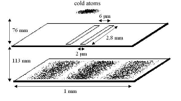
Figure 1: Schematic configuration of the experiment.

The first calculation of the wave function double slit experiment using electronsJonsson was done using the Feynman path integral method.Philippidis However, this calculation has some limitations. It covered only phenomena after the exit from the slits, and did not consider realistic slits. The slits, which could be well represented by a function $G(y)$ with $G(y)=1$ for $-\beta\leq y\leq\beta$ and $G(y)=0$ for $|y|>\beta$, were modeled by a Gaussian function $G(y)=e^{-y^{2}/2\beta^{2}}$. Interference was found, but the calculation could not account for diffraction at the edge of the slits. Another simulation with photons, with the same approximations, was done recently.Ghose Recently, some interesting simulations of the experiments on single and double slit diffraction of neutronsZeilinger_1988 were done.Sanz_2002

The simulations discussed here cover the entire experiment, beginning with a single source of atoms, and treat the slit realistically, also considering the initial dispersion of the velocity. We will use the Feynman path integral method to calculate the time-dependent wave function. The calculation and the results of the simulation are presented in Sec. II. The evolution of the probability density of the wave packet just after the slits raises the question of the interpretation of the wave/particle dualism. For this reason, it is interesting to simulate the trajectories in the de BrogliedeBroglie and BohmBohm formalism, which give a natural explanation of particle impacts. These trajectories are discussed in Sec. III.

II Calculation of the wave function with Feynman path integral

In the simulation we assume that the wave function of each source atom is Gaussian in $x$ and $y$ (the horizontal variables perpendicular and parallel to the slits) with a standard deviation $\sigma_{0}=\sigma_{x}=\sigma_{y}=10\,\mu$m. We also assume that the wave function is Gaussian in $z$ (the vertical variable) with zero average and a standard deviation $\sigma_{z}\simeq 0.3$ mm. The origin $(x=0,y=0,z=0)$ is at the center of the atomic source and the center of the Gaussian.

The small amount of vertical atomic dispersion compared to typical vertical distances, $\sim 100$ and 200 mm, allows us to make a few approximations. Each source atom has an initial velocity $\textbf{v}=(v_{0x},v_{0y},v_{0z})$ and wave vector $\textbf{k}=(k_{0x},k_{0y},k_{0z})$ defined as $\textbf{k}=m\textbf{v}/\hbar$. We choose a wave number at random according to a Gaussian distribution with zero average and a standard deviation $\sigma_{k}=\sigma_{k_{x}}=\sigma_{k_{y}}=\sigma_{k_{z}}=m\sigma_{v}/\sqrt{3}\hbar\simeq 2\times 10^{8}$ m^-1, corresponding to the horizontal and vertical dispersion of the atoms’ velocity inside the cloud (trap). For each atom with initial wave vector k, the wave function at time $t=0$ is

$$\psi_{0}(x,y,z;k_{0x},k_{0y},k_{0z}) = \psi_{0_{x}}(x;k_{0x})\psi_{0_{y}}(z;k_{0y})\psi_{0_{z}}(z;k_{0z})$$ (1)

$$= (2\pi\sigma_{0}^{2})^{-1/4}e^{-x^{2}/4\sigma_{0}^{2}}\,e^{ik_{0x}x}$$

$${}\times(2\pi\sigma_{0}^{2})^{-1/4}\,e^{-y^{2}/4\sigma_{0}^{2}}\,e^{ik_{0y}y}$$

$${}\times(2\pi\sigma_{z}^{2})^{-1/4}\,e^{-z^{2}/4\sigma_{z}^{2}}e^{ik_{0z}z}.$$

The calculation of the solutions to the Schrödinger equation were done with the Feynman path integral method,FeynmanQMI which defines an amplitude called the kernel. The kernel characterizes the trajectory of a particle starting from the point $\alpha=(x_{\alpha},y_{\alpha},z_{\alpha})$ at time $t_{\alpha}$ and arriving a at the point $\beta=(x_{\beta},y_{\beta},z_{\beta})$ at time $t_{\beta}$. The kernel is a sum of all possible trajectories between these two points and the times $t_{\alpha}$ and $t_{\beta}$.

Using the classical form of the Lagrangian

$$L(\dot{x},\dot{y},\dot{z},z,t)=m\frac{{\dot{x}}^{2}}{2}+m\,\frac{{\dot{y}}^{2}}{2}+m\frac{{\dot{z}}^{2}}{2}+mgz.$$ (2)

FeynmanFeynmanQMI defined the kernel by

$$K(\beta,t_{\beta};\alpha,t_{\alpha})\sim\exp\big{(}{\frac{i}{\hbar}S_{\rm cl}(\beta,t_{\beta};\alpha,t_{\alpha})}\big{)}=\exp\big{(}\frac{i}{\hbar}\!\int_{t_{\alpha}}^{t_{\beta}}L(\dot{x},\dot{y},\dot{z},z,t)\,dt\big{)},$$ (3)

with $\int_{-\infty}^{+\infty}\int_{-\infty}^{+\infty}K(\beta,t_{\beta};\alpha,t_{\alpha})\,dx_{\alpha}\,dy_{\alpha}\,dz_{\alpha}=1$. Hence,

$$K(\beta,t_{\beta};\alpha,t_{\alpha})=K_{x}(x_{\beta},t_{\beta};x_{\alpha},t_{\alpha})K_{y}(y_{\beta},t_{\beta};y_{\alpha},t_{\alpha})K_{z}(z_{\beta},t_{\beta};z_{\alpha},t_{\alpha}),$$ (4)

with

$$K_{x}(x_{\beta},t_{\beta};x_{\alpha},t_{\alpha}) = \Big{(}\frac{m}{2i\pi\hbar(t_{\beta}-t_{\alpha})}\Big{)}^{1/2}\exp{\frac{im}{\hbar}\Big{(}\frac{(x_{\beta}-x_{\alpha})^{2}}{2(t_{\beta}-t_{\alpha})}\Big{)}}$$ (5a)

$$K_{y}(y_{\beta},t_{\beta};y_{\alpha},t_{\alpha}) = \Big{(}\frac{m}{2i\pi\hbar(t_{\beta}-t_{\alpha})}\Big{)}^{1/2}\exp{\frac{im}{\hbar}\Big{(}\frac{(y_{\beta}-y_{\alpha})^{2}}{2(t_{\beta}-t_{\alpha})}\Big{)}}$$ (5b)

$$K_{z}(z_{\beta},t_{\beta};z_{\alpha},t_{\alpha}) = \Big{(}\frac{m}{2i\pi\hbar(t_{\beta}-t_{\alpha})}\Big{)}^{1/2}\exp{\frac{im}{\hbar}\Big{(}\frac{(z_{\beta}-z_{\alpha})^{2}}{2(t_{\beta}-t_{\alpha})}\Big{)}}.$$ (5c)

$$\times\exp{\frac{im}{\hbar}\Big{(}\frac{g}{2}(z_{\beta}+z_{\alpha})(t_{\beta}-t_{\alpha})-\frac{g^{2}}{24}(t_{\beta}-t_{\alpha})^{3}\Big{)}}.$$

For each atom with initial wave vector k, let us designate by $\psi(\alpha,t_{\alpha};\textbf{k})$ the wave function at time $t_{\alpha}$. We call S the set of points $\alpha$ where this wave function does not vanish. It is then possible to calculate the wave function at a later time $t_{\alpha}$ at points $\beta$ such that there exits a straight line connecting $\alpha$ and $\beta$ for any point $\alpha\in S$. In this case, FeynmanFeynmanQMI has shown that:

$$\psi(\beta,t;k_{0x},k_{0y},k_{0z})=\!\int_{(x_{\alpha},y_{\alpha},z_{\alpha})\in S}K(\beta,t;\alpha,t_{\alpha})\,\psi(\alpha,t_{\alpha};k_{0x},k_{0y},k_{0z})\,dx_{\alpha},dy_{\alpha},dz_{\alpha}.$$ (6)

For the double slit experiment, two steps are then necessary for the calculation of the wave function: a first step before the slits and a second step after the slits.

If we substitute Eqs. (1) and (4) in Eq. (6), we see that Feynman’s path integral allows a separation of variables, that is,

$$\psi(x,y,z,t;k_{0x},k_{0y},k_{0z})=\psi_{x}(x,t;k_{0x})\psi_{y}(y,t;k_{0y})\psi_{z}(z,t;k_{0z}).$$ (7)

References Shimizu, and Tannoudji, treat the vertical variable $z$ classically, which is shown in Appendix A to be a good approximation. Hence, we have $z(t)=z_{0}+v_{0z}t+gt^{2}/2$. The arrival time of the wave packet at the slits is $t_{1}(v_{0z},z_{0})=\sqrt{\frac{2(l_{1}-z_{0})}{g}+\big{(}\frac{v_{0z}}{g}\big{)}^{2}}-\frac{v_{0z}}{g}$. For $v_{0z}=0$ and $z_{0}=0$, we have $t_{1}=\sqrt{\frac{2l_{1}}{g}}=124$ ms and the atoms have been accelerated to $v_{z1}=gt_{1}=1.22$ m/s on average at the slit. Thus the de Broglie wavelength $\lambda=\hbar/mv_{z1}=1.8\times 10^{-8}$ m is two orders of magnitude smaller than the slit width, $2\mu m$.

Because the two slits are very long compared with their other dimensions, we will assume they are infinitely long, and there is no spatial constraint on $y$. Hence, we have for an initial fixed velocity $v_{0y}$:

$$\psi_{y}(y,t;k_{0y})=\!\int_{y_{\alpha}}K_{y}(y,t;y_{\alpha},t_{\alpha}=0)\psi_{0}(y_{\alpha};k_{0y})\,dy_{\alpha}.$$ (8)

Thus

$$\psi_{y}(y,t;k_{0y})=(2\pi s_{0}^{2}(t))^{-1/4}\exp[-\frac{(y-v_{0y}t)^{2}}{4\sigma_{0}s_{0}(t)}+ik_{0y}(y-v_{0y}t)],$$ (9)

with $s_{0}(t)=\sigma_{0}(1+\frac{i\hbar t}{2m\sigma_{0}^{2}})$.

The wave packet is an infinite sum of wavepackets with fixed initial velocity. The probability density as a function of $y$ is

$$\rho_{y}(y,t)=\!\int_{-\infty}^{+\infty}(2\pi\tau^{2})^{-1/2}e^{-k_{y}^{2}/2\tau^{2}}|\psi_{y}(y,t;k_{y})|^{2}\,dk_{y}=(2\pi\varepsilon_{0}^{2}(t))^{-1/2}\,e^{-y^{2}/2\varepsilon_{0}^{2}(t)},$$ (10)

with $\varepsilon_{0}^{2}(t)=\sigma_{0}^{2}(t)+(\frac{\hbar t\tau}{m})^{2}$ and $\sigma_{0}^{2}(t)=\sigma_{0}^{2}+(\frac{\hbar t}{2m\sigma_{0}^{2}})^{2}$. Because we know the dependence of the probability density on $y$, in what follows we consider only the wave function $\psi_{x}(x,t;k_{0x})$.

II.1 The wave function before the slits

Before the slits, we have

$$\psi_{x}(x,t;k_{0x}) = (2\pi s_{0}^{2}(t))^{-1/4}\exp\big{[}-\frac{(x-v_{0x}t)^{2}}{4\sigma_{0}s_{0}(t)}+ik_{0x}(x-v_{0x}t)\big{]}$$ (11)

$$\rho_{x}(x,t) = (2\pi\varepsilon_{0}^{2}(t))^{-1/2}\exp\big{[}-\frac{x^{2}}{2\varepsilon_{0}^{2}(t)}\big{]}.$$ (12)

It is interesting that the scattering of the wave packet in $x$ is caused by the dispersion of the initial position $\sigma_{0}$ and by the dispersion $\tau$ of the initial velocity $v_{0x}$ (see Fig. 2). Only 0.1% of the atoms will cross through one of the slits; the others will be stopped by the plate.

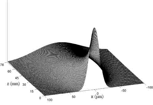
Figure 2: Evolution of the density $\rho_{x}(x,t)$ before the slits, The time of the scattering of the initial wave packet ($t$ is determined from $z=z_{0}+v_{0z}t+\frac{gt^{2}}{2}$).

II.2 The wave function after the slits

The wave function after the slits with fixed $z_{0}$ and $k_{0z}=mv_{0z}/\hbar$ for $t\geq t_{1}(v_{0z},z_{0})$ is deduced from the values of the wave function at slits A and B (cf.Fig. 3) by using Eq. (6). We obtain:

$$\psi_{x}(x,t;k_{0x},k_{0z},z_{0})=\psi_{A}+\psi_{B},$$ (13)

with

$$\psi_{A}=\!\int_{A}K_{x}(x,t;x_{a},t_{1}(v_{0z},z_{0}))\,\psi_{x}(x_{a},t_{1}(v_{0z},z_{0});k_{0x})\,dx_{a}$$ (14a)

$$\psi_{B}=\!\int_{B}K_{x}(x,t;x_{b},t_{1}(v_{0z},z_{0}))\,\psi_{x}(x_{b},t_{1}(v_{0z},z_{0});k_{0x})\,dx_{b},$$ (14b)

where $\psi_{x}(x_{a},t_{1}(v_{0z},z_{0});k_{0x})$ and $\psi_{x}(x_{b},t_{1}(v_{0z},z_{0});k_{0x})$ are given by Eq. (11) whereas $K_{x}(x,t;x_{a},t_{1}(v_{0z},z_{0}))$ and $K_{x}(x,t;x_{b},t_{1}(v_{0z},z_{0}))$ are given by Eq. (5a).

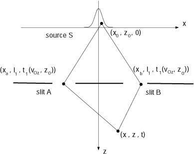
Figure 3: Schematic representation of the experiment: calculation method of the wave function after the slits.

The probability density is

$$\rho_{x}(x,t;k_{0z},z_{0})=\!\int_{-\infty}^{+\infty}(2\pi\tau^{2})^{-1/2}\exp\Big{(}-\frac{k_{0x}^{2}}{2\tau^{2}}\Big{)}|\psi_{x}(x,t;k_{0x},k_{0z},z_{0})|^{2}\,dk_{0x}.$$ (15)

The arrival time $t_{2}$ of the center of the wave packet on the detecting plate depends on $z_{0}$ and $v_{0z}$. We have $t_{2}=\sqrt{\frac{2(l_{1}+l_{2}-z_{0})}{g}+\big{(}\frac{v_{0z}}{g}\big{)}^{2}}-\frac{v_{0z}}{g}$. For $z_{0}=0$ and $v_{0z}=0$, $t_{2}=\sqrt{\frac{2(l_{1}+l_{2})}{g}}=196$ ms and the atoms are accelerated to $v_{z2}=gt_{2}=1.93$ m/s.

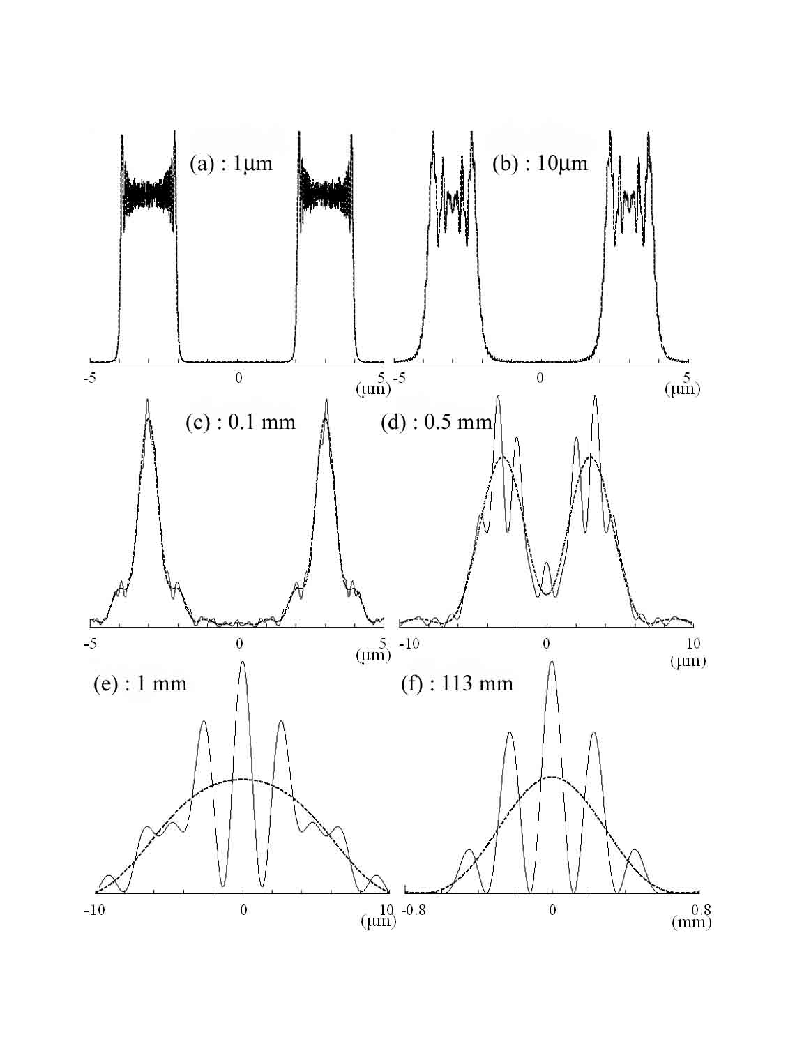
Figure 4: Comparison between $|\psi_{A}+\psi_{B}|^{2}$ (plain line) and $|\psi_{A}|^{2}+|\psi_{B}|^{2}$ (dotted line) with $z_{0}=0$ and $k_{0z}=0$ at (a) $1\,\mu$m, (b) $10\,\mu$ m, (c) 0.1 mm, (d) 0.5 mm, (e) 1 mm, and (f) 113 mm after the slits.

The calculation of $\rho_{x}(x,t;k_{0z},z_{0})$ at any $(x,t)$ with $k_{0z}$ and $z_{0}$ given and $t\geq t_{1}$ is done by a double numerical integration: (a) Eq. (15) is integrated numerically using a discretization of $k_{0x}$ into 20 values; (b) the integration of Eq. (13) using Eqs. (14) is done by a discretization of the slits $A$ and $B$ into 200 values each. Figure 4 shows the cross sections of the probability density ($|\psi_{A}+\psi_{B}|^{2}$) for $z_{0}=0$, $v_{0z}=0$ $(k_{0z}=0)$ and for several distances ($\Delta z=\frac{1}{2}gt^{2}-\frac{1}{2}gt_{1}^{2}$) after the double slit: $1\,\mu$m, $10\,\mu$ m, 0.1 mm, 0.5 mm, 1 mm and 113 mm.

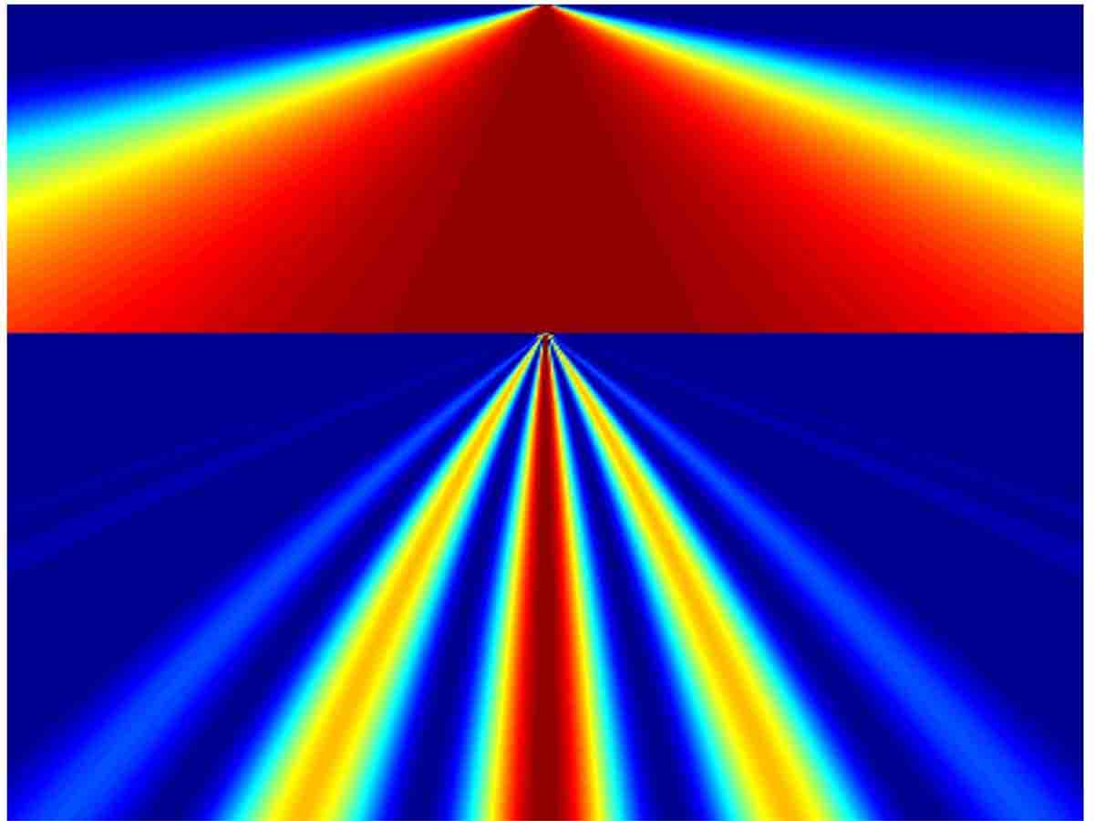
Figure 5: Evolution of the probability density $\rho_{x}(x,t;k_{0z}=0,z_{0}=0)$ from the source to the detector screen.

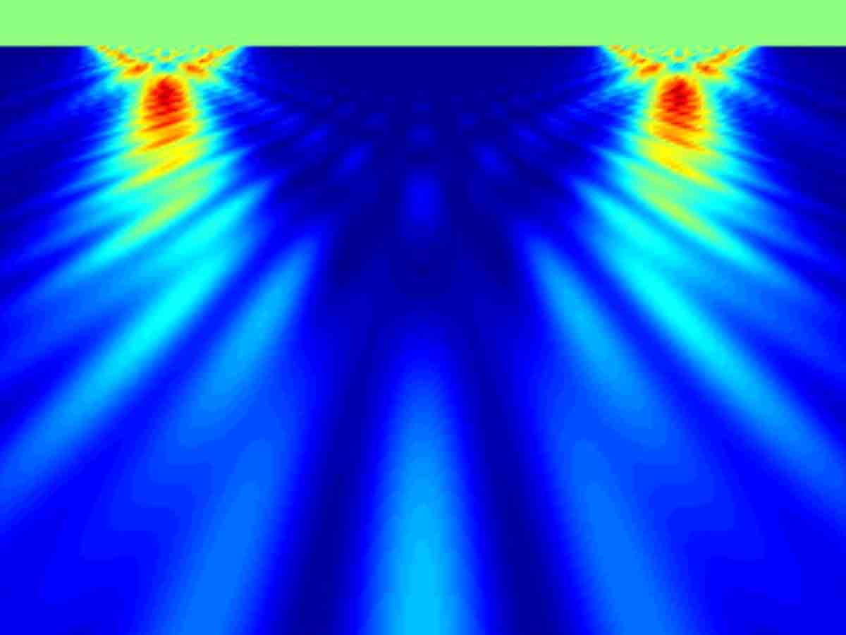
Figure 6: Evolution of the probability density $\rho_{x}(x,t;k_{0z}=0,z_{0}=0)$ for the first millimeter after the slits.

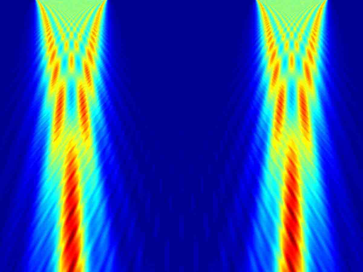
Figure 7: Evolution of the probability density $\rho_{x}(x,t;k_{0z}=0,z_{0}=0)$ for the first 100 $\mu$m after the slits.

The calculation method enables us to compare the evolution of the probability density when both slits are simultaneously open (interference: $|\psi_{A}+\psi_{B}|^{2}$) with the sum of the evolutions of the probability density when the two slits are successively opened (sum of two diffraction phenomena: ($|\psi_{A}|^{2}+|\psi_{B}|^{2}$). Figure 4 shows the probability density ($|\psi_{A}|^{2}+|\psi_{B}|^{2}$) for the same cases. Note that the difference between the two phenomena does not exist immediately at the exit of the two slits; differences appear only after some millimeters after the slits.

Figures 5–7 show the evolution of the probability density. At 0.1 mm after the slits, we know through which slit each atom has passed, and thus the interference phenomenon does not yet exist (see Figs. 4 and 7). Only at 1 mm after the slits do the interference fringes become visible, just as we would expect by the Fraunhoffer approximation (see Figs. 4 and 6).

II.3 Comparison with the Shimizu experiment

In the Shimizu experiment, atoms arrive at the detection screen between $t=t_{\min}$ and $t_{\max}$. To obtain the measured probability density in this time interval, we have to sum the probability density above the initial position $z_{0}$ and their initial velocity $v_{0z}$ compatible with $t_{\min}\leq t_{2}\leq t_{\max}$, that is,

$$\rho_{x}(x,t_{\min}\leq t\leq t_{\max})=\!\int_{t_{\min}\leq t_{2}\leq t_{\max}}\rho_{x}(x,t_{2};k_{0z},z_{0})\,e^{-k_{0z}^{2}/2\tau^{2}}e^{-z_{0}^{2}/2\sigma_{z}^{2}}\,dk_{0z}dz_{0}.$$ (16)

The positions at the detection screen can only be measured to about 80 $\mu$m, and thus to compare our results with the measured results. we perform the average

$$\rho_{\rm measured}(x,t_{\min}\leq t\leq t_{\max})=\frac{1}{80\,\mu\rm m}\!\int_{x-40\mu m}^{x+40\mu m}\rho(u,t_{\min}\leq t\leq t_{\max})\,du.$$ (17)

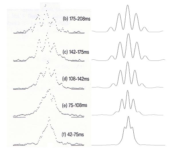
Figure 8: Comparison of the probability density measured experimentally by ShimizuShimizu (left) and the probability density calculated numerically with our model (right).

Figure 8 compares those calculations to the results found in Ref. Shimizu, . The experimental fringe separation is narrower than in our calculation, see Figs. 8 and 11. This difference is explained by a technical problem in the Shimizu experiment.Shimizu

III Impacts on screen and trajectories

In the Shimizu experiment the interference fringes are observed through the impacts of the neon atoms on a detection screen. It is interesting to simulate the neon atoms trajectories in the de Broglie-Bohm interpretation,deBroglie ; Bohm which accounts for atom impacts. In this formulation of quantum mechanics, the particle is represented not only by its wave function, but also by the position of its center of mass. The atoms have trajectories which are defined by the speed $\textbf{v}(x,y,z,t)$ of the center of mass, which at position $(x,y,z)$ at time $t$ is given byHolland ; GondranMA

$$\textbf{v}(x,y,z,t)=\frac{\nabla S(x,y,z,t)}{m}+\frac{\nabla\log\rho(x,y,z,t)\times\textbf{s}}{m}=\frac{\hbar}{m\rho}[{\rm Im}(\psi^{*}\nabla\psi)+{\rm Re}(\psi^{*}\nabla\psi)\times\frac{\textbf{s}}{|\textbf{s}|}],$$ (18)

where $\psi(x,y,z,t)=\sqrt{\rho(x,y,z,t)}\exp{\left(\frac{i}{\hbar}S(x,y,z,t)\right)}$ and s is the spin of the particle. Let us see how this interpretation gives the same experimental results as the Copenhagen interpretation.

If $\psi$ satisfies the Schrödinger equation,

$$i\hbar\frac{\partial\psi}{\partial t}=-\frac{\hbar^{2}}{2m}\nabla^{2}\psi+V\psi,$$ (19)

with the initial condition $\psi(x,y,z,0)=\psi_{0}(x,y,z)=\sqrt{\rho_{0}(x,y,z)}\exp(\frac{i}{\hbar}S_{0}(x,y,z))$, then $\rho$ and $S$ satisfy:

$$\frac{\partial S}{\partial t}+\frac{1}{2m}(\nabla S)^{2}+V-\frac{\hbar^{2}}{2m}\frac{\triangle\sqrt{\rho}}{\sqrt{\rho}} = 0$$ (20)

$$\frac{\partial\rho}{\partial t}+\nabla\cdot\Big{(}\rho\frac{\nabla S}{m}\Big{)} = 0,$$ (21)

with initial conditions $S(x,y,z,0)=S_{0}(x,y,z)$ and $\rho(x,y,z,0)=\rho_{0}(x,y,z)$.

In both interpretations, $\rho(x,y,z,t)=|\psi(x,y,z,t)|^{2}$ is the probability density of the particles. But, in the Copenhagen interpretation, it is a postulate for each $t$ (confirmed by experience). In the de Broglie-Bohm interpretation, if $\rho_{0}(x,y,z)$ is the probability density of presence of particles for $t=0$ only, then $\rho(x,y,z,t)$ must be the probability density of the presence of particles without any postulate because Eq. (21) becomes the Madelung equation:

$$\frac{\partial\rho}{\partial t}+\nabla\cdot(\rho\textbf{v})=0,$$ (22)

(thanks to $\textbf{v}=\frac{\nabla S}{m}+\nabla\times(\frac{\ln\rho}{m})\textbf{s}$), which is obviously the fluid mechanics equation of conservation of the density. The two interpretations therefore yield statistically identical results. Moreover, the de Broglie-Bohm theory naturally explains the individual impacts.

In the initial de Broglie-Bohm interpretation,deBroglie ; Bohm which was not relativistic invariant, the velocity was not given by Eq. (18), but by $\textbf{v}=\frac{\nabla S}{m}$ which does not involve the spin. In the Shimizu experiment, the spin of each neon atom in the magnetic trap was constant and vertical: $\textbf{s}=(0,0,\frac{\hbar}{2})$. In our case the spin-dependent term $\frac{\nabla\log\rho}{m}\times\textbf{s}=\frac{\hbar}{2m\rho}\big{(}\frac{\partial\rho}{\partial y},-\frac{\partial\rho}{\partial x},0\big{)}$ is negligible after the slit, but not before.

For the simulation, we choose at random (from a normal distribution $f(0,0,0;\sigma_{k},\sigma_{k},\sigma_{k})$ the wave vector $\textbf{k}=(k_{0x},k_{0y},k_{0z})$ to define the initial wave function (1) of the atom prepared inside the magneto-optic trap. For the de Broglie-Bohm interpretation, we also choose at random the initial position $(x_{0},y_{0},z_{0})$ of the particle inside its wave packet (normal distribution $f((0,0,0);(\sigma_{0},\sigma_{0},\sigma_{z}))$). The trajectories are given by

$$\frac{dx}{dt} = v_{x}(x,t)=\frac{1}{m}\frac{\partial S}{\partial x}+\frac{\hbar}{2m\rho}\frac{\partial\rho}{\partial y}$$ (23a)

$$\frac{dy}{dt} = v_{y}(x,t)=\frac{1}{m}\frac{\partial S}{\partial y}-\frac{\hbar}{2m\rho}\frac{\partial\rho}{\partial x}$$ (23b)

$$\frac{dz}{dt} = v_{z}(x,t)=\frac{1}{m}\frac{\partial S}{\partial z},$$ (23c)

where $\rho(x,y,t;k_{0x},k_{0y})=|\psi_{x}(x,t;k_{0x})\psi_{y}(y,t;k_{0y})|^{2}$ and $\psi_{x}$ and $\psi_{y}$ are given by Eqs. (9)–(13).

III.1 Trajectories before the slits

Before the slits, Appendix B gives $z(t)=z_{0}\frac{\sigma_{z}(t)}{\sigma_{z}}+v_{0z}t+\frac{1}{2}gt^{2}$, $x(t)=v_{0x}t+\sqrt{x_{0}^{2}+y_{0}^{2}}\frac{\sigma_{0}(t)}{\sigma_{0}}\cos{\varphi(t)}$, and $y(t)=v_{0y}t+\sqrt{x_{0}^{2}+y_{0}^{2}}\frac{\sigma_{0}(t)}{\sigma_{0}}\sin{\varphi(t)}$, with $\varphi(t)=\varphi_{0}+{\rm arctan}\big{(}-\frac{\hbar t}{2m\sigma_{0}^{2}}\big{)}$, $\cos\varphi_{0}=\frac{x_{0}}{\sqrt{x_{0}^{2}+y_{0}^{2}}}$ and $\sin\varphi_{0}=\frac{y_{0}}{\sqrt{x_{0}^{2}+y_{0}^{2}}}$. For a given wave vector k and an initial position $(x_{0},y_{0},z_{0})$ inside the wave packet, an atom of neon will arrive at a given position on the plate containing the slits. Notice that the term $\nabla\log\rho\times\textbf{s}/m$ adds to the trajectory defined by $\nabla S/m$ a rotation of $-\pi/2$ around the spin axis (the $z$ axis).

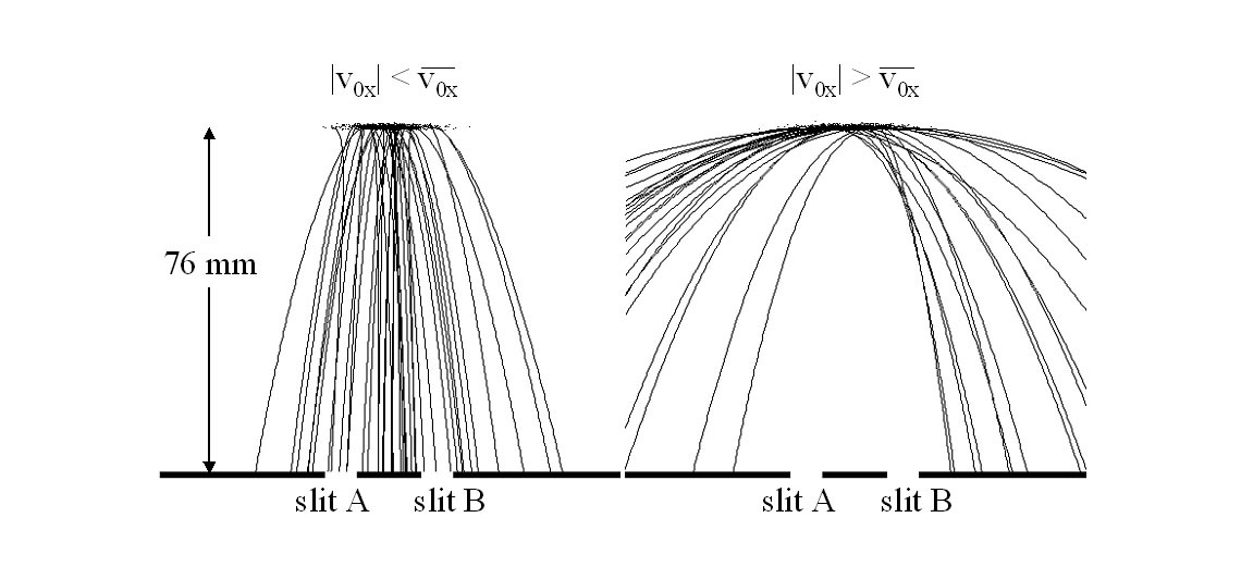
Figure 9: Trajectories of atoms before the slit. Note that if the initial velocities $|v_{0x}|\geq 3.9\times 10^{-4}$ m/s, then no atoms can cross the slit.

The source atoms do not all pass through the slits; most of them are stopped by the plate. Only atoms having a small horizontal velocity $v_{0x}$ can go through the slits. Indeed an atom with an initial velocity $v_{0x}$ and an initial position $x_{0},y_{0}$ arrives at the slits at $t=t_{1}$ at the horizontal position $x(t_{1})=v_{0x}t_{1}+y_{0}(\sigma_{0}(t_{1})/\sigma_{0})$. For this atom to go through one of the slits, it is necessary that $|x(t_{1})|\leq\overline{x}$, with $\overline{x}=(d+b)/2=4\times 10^{-6}$ m and $-2\sigma_{0}\leq y_{0}\leq 2\sigma_{0}$ and $t_{1}\simeq 0.124$ s. Consequently, it is necessary that the initial velocities of the atoms satisfy $|v_{0x}|\leq(\overline{x}+2\sigma_{0}(t_{1}))/t_{1}=\overline{v}_{0x}\simeq 3.9\times 10^{-4}$ m/s. The double slit filters the initial horizontal velocities and transforms the source atoms after the slits into a quasi-monochromatic source. The horizontal velocity of an atom leads to a horizontal shift of the atom’s impacts on the detection screen. The maximum shift is $\Delta x=\overline{v}_{0x}\Delta t$, where $\Delta t$ is the time for the atom to go from the slits to the screen ($\Delta t=t_{2}-t_{1}\simeq 0.072$ s); hence $\Delta x\simeq 2.8\times 10^{-5}$ m. This shift does not produce a blurring of the interference fringes because the interference fringes are separated from one another by $25\times 10^{-5}\,{\rm m}\gg\Delta x$. Note that if the source was nearer to the double slit (for example if $l_{1}=5$ mm, then $\Delta x\simeq 10\times 10^{-5}$ m), the slit would not filter enough horizontal velocities and consequently the interference fringes would not be visible.

The system appears fully deterministic. If we know the position and the velocity of an atom inside the source, then we know if it can go through the slit or not. Figure 9 shows some trajectories of the source atoms as a function of their initial velocities. Only atoms with a velocity $|v_{0x}|\leq\overline{v}_{0x}$ can go through the slits.

III.2 Velocities and trajectories after the slits

In what follows, we consider only atoms that have gone through one of the slits. After the slits, we still have $z(t)=v_{0z}t+\frac{1}{2}gt^{2}+z_{0}(\sigma_{z}(t)/\sigma_{z})$, but now $v_{x}(t)$ and $v_{y}(t)$ and $x(t)$ and $y(t)$ have to be calculated numerically. The calculation of $v_{x}(x,t)$ is done by a numerical computation of an integral in $x$ above the slits A and B (see Appendix B); $x(t)$ is calculated with a Runge-Kutta method.Lambert We use a time step $\Delta t$ which is inversely proportional to the acceleration. At the exit of the slit, $\Delta t$ is very small: $\Delta t\simeq 10^{-8}$ s; it increases to $\Delta t\simeq 10^{-4}$ s at the detection screen. Figure 10 shows the trajectories of the atoms just after the slits; $x_{0}$ and $y_{0}$ are drawn at random, $z_{0}=0$, with $v_{0x}=v_{0z}=0$.

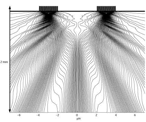
Figure 10: Zoom of trajectories of atoms for the first millimeters after the slit ($k_{0x}=k_{0z}=0$).

III.3 Impacts on the screen

We observe the impact of each particle on the detection screen as shown by the last image in Fig. 11. The classic explanation of these individual impacts on the screen is the reduction of the wave packet. An alternative interpretation is that the impacts are due to the decoherence caused by the interaction with the measurement apparatus.

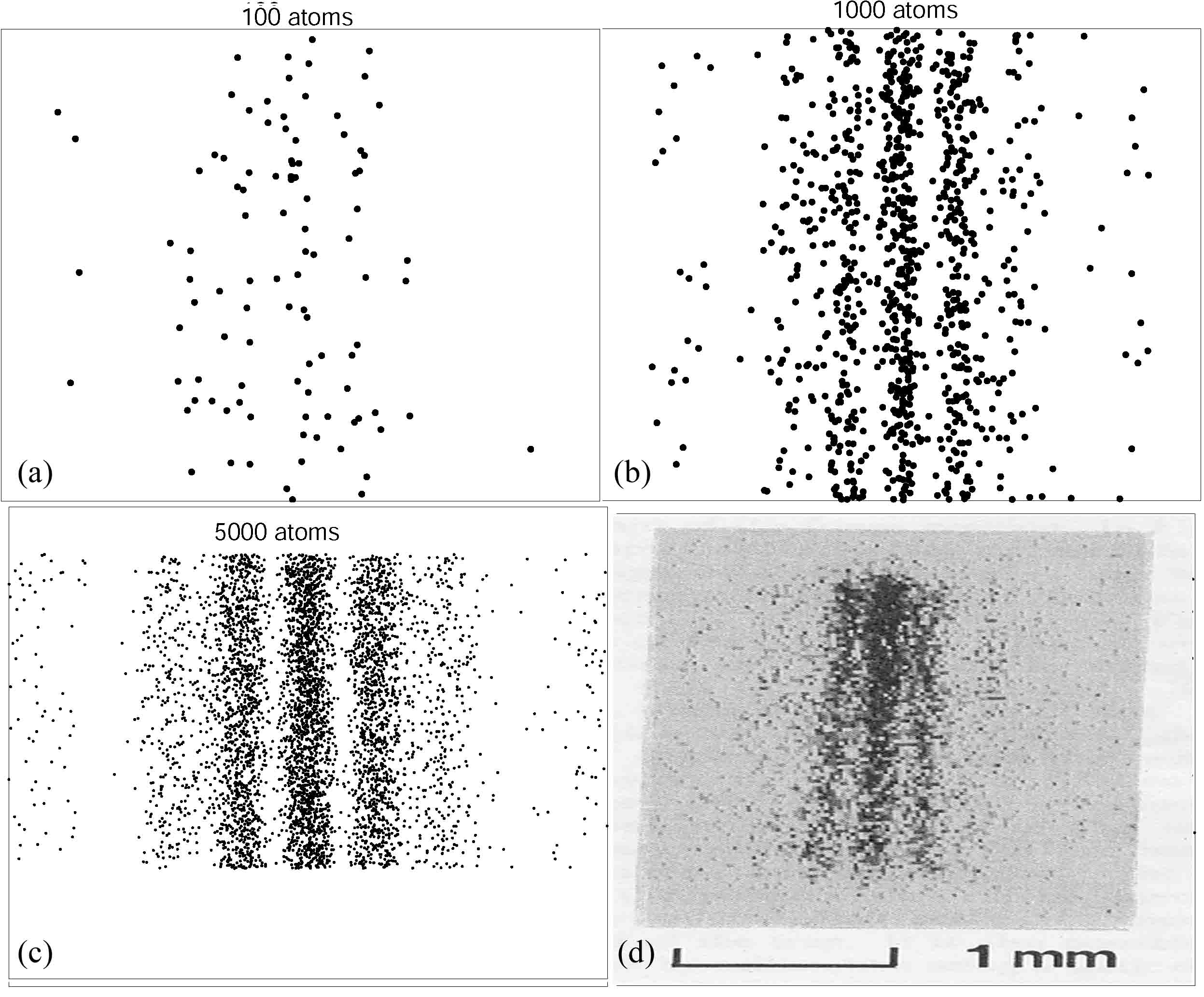
Figure 11: Atomic impacts on the screen of detection.

In the de Broglie-Bohm formulation of quantum mechanics, the impact on the screen is the position of the center of mass of the particle, just as in classical mechanics. Figure 11 shows our results for 100, 1000, and 5000 atoms whose initial position $(x_{0},y_{0},z_{0})$ are drawn at random. The last image corresponds to 6000 impacts of the Shimizu experiment.Shimizu The simulations show that it is possible to interpret the phenomena of interference fringes as a statistical consequence of a particle trajectories.

IV Summary

We have discussed a simulation of the double slit experiment from the source of emission, passing through a realistic double slit, and its arrival at the detector. This simulation is based on the solution of Schrödinger’s equation using the Feynman path integral method. A simulation with the parameters of the 1992 Shimizu experiment produces results consistent with their observations. Moreover the simulation provides a detailed description of the phenomenon in the space just after the slits, and shows that interference begins only after 0.5 mm. We also show that it is possible to simulate the trajectories of particles by using the de Broglie-Bohm interpretation of quantum mechanics.

Appendix A Calculation of $\psi_{z}(z,t;k_{0z})$

Because there is no constraints on the vertical variable $z$, we find using Eqs. (5c) and (6) for all $t>0$ (before and after the double slit) that

$$\psi_{z}(z,t;k_{0z})=\!\int_{S}\!K_{z}(z,t;z_{\alpha},t=0)\times\psi_{0_{z}}(z_{\alpha};k_{0z})\,dz_{\alpha},$$ (24)

where the integration is done over the set S of the points $z_{\alpha}$ where the initial wave packet $\psi_{0_{z}}(z_{\alpha};k_{0z})$ does not vanish. We obtain:

$$\psi_{z}(z,t;k_{0z}) = (2\pi s_{z}^{2}(t))^{-1/4}\exp\Big{(}-\frac{(z-v_{0z}t-gt^{2}/2)^{2}}{4\sigma_{z}s_{z}(t)}\Big{)}$$ (25)

$$\times\exp\Big{[}\frac{im}{\hbar}\big{(}(v_{0z}+gt)(z-v_{0z}t/2)-\frac{mg^{2}t^{3}}{6}\big{)}\Big{]},$$

where $s_{z}(t)=\sigma_{z}\big{(}1+\frac{i\hbar t}{2m\sigma_{z}^{2}}\big{)}$. Consequently we have:

$$|\psi_{z}(z,t;v_{0z})|^{2}=(2\pi\sigma_{z}^{2}(t))^{-1/2}\exp\Big{[}-\frac{(z-v_{0z}t-gt^{2}/2)^{2}}{2\sigma_{z}^{2}(t)}\Big{]},$$ (26)

with $\sigma_{z}(t)=|s_{z}(t)|=\sigma_{z}\big{(}1+\big{(}\frac{\hbar t}{2m\sigma_{z}^{2}}\big{)}^{2}\big{)}^{1/2}$.

Note that $\sigma_{z}(t)$ is negligible compared to $l_{1}$ ($\sigma_{z}=0.3\,$mm and $\frac{\hbar t}{2m\sigma_{z}}=10^{-3}$ mm are negligible compared to $l_{1}=76$ mm for an average crossing time inside the interferometer of $t\sim 200$ ms). Therefore $(2\pi\sigma_{z}^{2}(t))^{-1/2}\exp\big{[}-\frac{(z-v_{0z}t-gt^{2}/2)^{2}}{2\sigma_{z}^{2}(t)}\big{]}\simeq\delta_{0}(z-v_{0z}t-\frac{gt^{2}}{2})$, and if $z_{0}$ is the initial position of the particle, we have $z\simeq z_{0}+v_{0z}t+\frac{gt^{2}}{2}$ at time $t$.

Appendix B Calculation of the atom’s trajectories

The velocity (18) applied to Eq. (25) gives the differential equation for the vertical variable $z$,

$$\frac{dz}{dt}=v_{z}(z,t)=\frac{1}{m}\frac{\partial S}{\partial z}=v_{0z}+gt+\frac{(z-v_{0z}t-gt^{2}/2)\hbar^{2}t}{4m^{2}\sigma_{z}^{2}\sigma_{z}^{2}(t)},$$ (27)

from which we find

$$z(t)=v_{0z}t+\frac{1}{2}gt^{2}+z_{0}\frac{\sigma_{z}(t)}{\sigma_{z}}.$$ (28)

Equation (28) gives the classical trajectory if $z_{0}=0$ (the center of the wave packet).

The velocity (18) applied before the slit to Eqs. (9) and (11) gives the differential equations in the $x$ and $y$ directions:

$$\frac{dx}{dt} = v_{x}(x,t)=\frac{1}{m}\frac{\partial S}{\partial x}+\frac{\hbar}{2m\rho}\frac{\partial\rho}{\partial y}=v_{0x}+\frac{(x-v_{0x}t)\hbar^{2}t}{4m^{2}\sigma_{0}^{2}\sigma_{0}^{2}(t)}-\frac{\hbar(y-v_{0y}t)}{2m\sigma_{0}^{2}(t)}$$ (29a)

$$\frac{dy}{dt} = v_{y}(x,t)=\frac{1}{m}\frac{\partial S}{\partial y}-\frac{\hbar}{2m\rho}\frac{\partial\rho}{\partial x}=v_{0y}-\frac{(y-v_{0y}t)\hbar^{2}t}{4m^{2}\sigma_{0}^{2}\sigma_{0}^{2}(t)}+\frac{\hbar(x-v_{0x}t)}{2m\sigma_{0}^{2}(t)}.$$ (29b)

It then follows that

$$x(t) = v_{0x}t+\sqrt{x_{0}^{2}+y_{0}^{2}}\frac{\sigma_{0}(t)}{\sigma_{0}}\cos{\varphi(t)}$$ (30a)

$$y(t) = v_{0y}t+\sqrt{x_{0}^{2}+y_{0}^{2}}\frac{\sigma_{0}(t)}{\sigma_{0}}\sin{\varphi(t)},$$ (30b)

with $\varphi(t)=\varphi_{0}+{\rm arctan}\big{(}-\frac{\hbar t}{2m\sigma_{0}^{2}}\big{)}$, $\cos(\varphi_{0})=\frac{x_{0}}{\sqrt{x_{0}^{2}+y_{0}^{2}}}$, and $\sin(\varphi_{0})=\frac{y_{0}}{\sqrt{x_{0}^{2}+y_{0}^{2}}}$. Equations (30a) and (30b) give the classical trajectory if $x_{0}=y_{0}=0$ (the center of the wave packet).

After the slits, the velocity $v_{x}(x,t)=\frac{\hbar}{m}\frac{Im(\frac{\partial\psi}{\partial x}\psi^{*})}{\psi\psi^{*}}$ given by Eq. (18) can be calculated using Eqs. (6), (14a) and (14b). We obtain:

$$v_{x}(x,t)=\frac{1}{t-t_{1}}\left[x+\frac{-1}{2(\alpha^{2}+\beta_{t}^{2})}\left(\beta_{t}Im\left(\frac{C(x,t)}{H(x,t)}\right)+\alpha Re\left(\frac{C(x,t)}{H(x,t)}\right)-\beta_{t}\gamma_{x,t}\right)\right]$$

with

$$H(x,t)=\int_{X_{A}-b}^{X_{A}+b}f(x,u,t)\,du+\int_{X_{B}-b}^{X_{B}+b}f(x,u,t)\,du$$

$$C(x,t)=\left[f(x,u,t)\right]_{u=X_{A}-b}^{u=X_{A}+b}+\left[f(x,u,t)\right]_{u=X_{B}-b}^{u=X_{B}+b}$$

where $X_{A}$ and $X_{B}$ are the centers of the two slits, and where

$$f(x,u,t)=\exp{[(\alpha+i\beta_{t})u^{2}+i\gamma_{x,t}u]}$$

$$\alpha=-\frac{1}{4\sigma_{0}^{2}\left(1+\left(\frac{\hbar t_{1}}{2m\sigma_{0}^{2}}\right)^{2}\right)}$$

$$\beta_{t}=\frac{m}{2\hbar}\left(\frac{1}{t-t_{1}}+\frac{1}{t_{1}\left(1+\left(\frac{2m\sigma_{0}^{2}}{\hbar t_{1}}\right)^{2}\right)}\right)$$

$$\gamma_{x,t}=-\frac{mx}{\hbar(t-t_{1})}.$$

Appendix C Convergence

In simulation, it is possible to make the Planck constant $h$ tend towards zero. So, it is possible to show, about the example of the Young slits, the convergence of the quantum mechanics to the classical mechanics. In the following simulations, one take $k_{0x}=k_{0z}=0$.

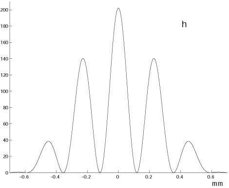
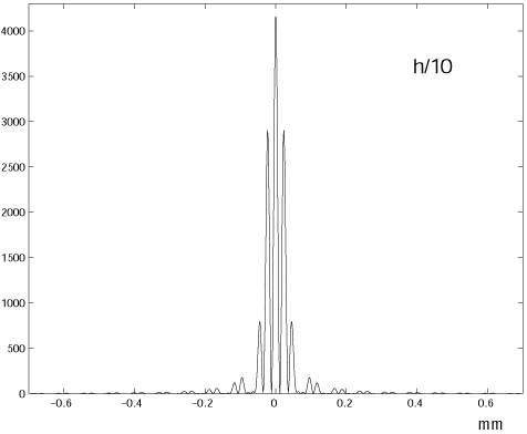
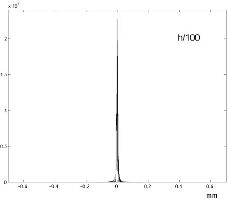
Figure 12: Cross section of the probability density on the screen of detection when $h$ is divided by 5, 10 and 100.

The figure 12 shows, when $h$ is divided by 100, how the interference fringes are getting strongly more and more narrow up to the distance between the slits.

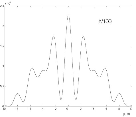
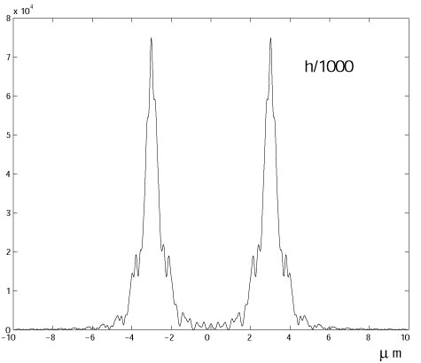
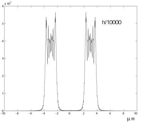
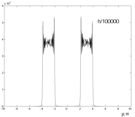
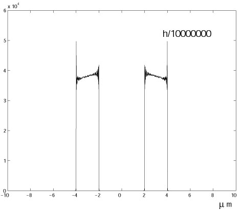
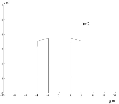
Figure 13: Cross section of the probability density on the screen of detection when $h$ tends towards zero.

The figure 13 shows, when $h$ is divided by 1000, that the interference fringes disappear and the probability density converges on the classical probability density ($h=0$).

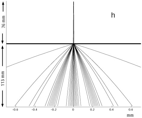
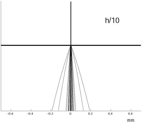
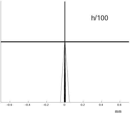
Figure 14: Trajectories of atoms for whole experience when $h$ is divided by 5, 10 and 100

The figure 14 shows how the trajectories become strongly narrower when $h$ is divided by 100.

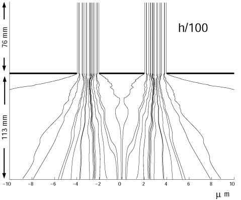
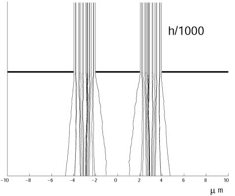
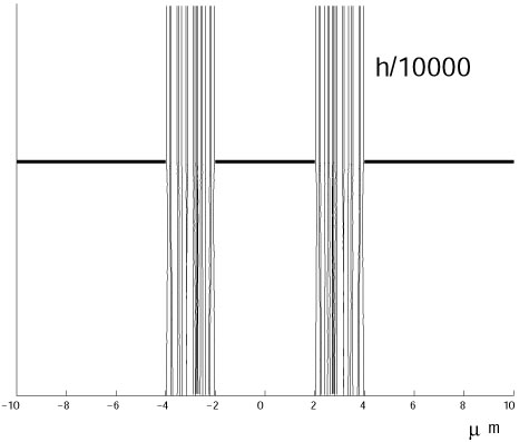
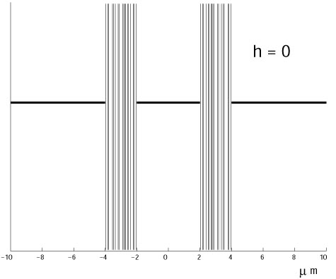
Figure 15: Trajectories of atoms for whole experience when $h$ tends towards zero.

The figure 15 clearly shows the convergence of the quantum trajectories to the classical trajectories ($h=0$).

After showing results of the evolution of the probability density and of the trajectories of atoms, it is difficult to throw down the hypothesis of trajectory.

Everything seems to happen also as if atoms have well a trajectory.

- (1) T. Young, ”On the theory of light and colors,” Philos. Trans. RSL 92, 12–48 (1802).
- (2) R. P. Feynman, R. B. Leighton, and M. Sands,The Feynman Lectures on Physics (Addison-Wesley, Reading, 1966), Vol. 3.
- (3) C. J. Davisson and L. H. Germer, “The scattering of electrons by a single crystal of nickel,” Nature 119, 558–560 (1927).
- (4) C. Jönsson, “Elektroneninterferenzen an mehreren künstlich hergestellten Feinspalten,” Z. Phy. 161, 454–474 (1961), English translation “Electron diffraction at multiple slits,” Am. J. Phys. 42, 4–11 (1974).
- (5) P. G. Merlin, C. F. Missiroli, and G. Pozzi, “On the statistical aspect of electron interference phenomena,” Am. J. Phys. 44, 306–307 (1976).
- (6) A. Tonomura, J. Endo, T. Matsuda, T. Kawasaki, and H. Ezawa, “Demonstration of single-electron buildup of an interference pattern,” Am. J. Phys. 57, 117–120 (1989).
- (7) H. V. Halbon Jr. and P. Preiswerk, “Preuve expérimentale de la diffraction des neutrons,” C. R. Acad. Sci. Paris 203, 73–75 (1936).
- (8) H. Rauch and A. Werner, Neutron Interferometry: Lessons in Experimental Quantum Mechanics (Oxford Univ. Press, London, 2000).
- (9) A. Zeilinger, R. Gähler, C. G. Shull, W. Treimer, and W. Mampe, “Single and double slit diffraction of neutrons,” Rev. Mod. Phys. 60, 1067–1073 (1988).
- (10) I. Estermann and O. Stern,“Beugung von Molekularstrahlen,” Z. Phy. 61, 95–125 (1930).
- (11) F. Shimizu, K. Shimizu, and H. Takuma, “Double-slit interference with ultracold metastable neon atoms,” Phys. Rev. A 46, R17–R20 (1992).
- (12) M. H. Anderson, J. R. Ensher, M. R. Mattheus, C. E. Wieman, and E. A. Cornell, “Observation of Bose-Einstein condensation in a dilute atomic vapor,” Science 269, 198–201 (1995).
- (13) M. Arndt, O. Nairz, J. Voss-Andreae, C. Keller, G. van des Zouw, and A. Zeilinger, “Wave-particle duality of C60 molecules,” Nature 401, 680–682 (1999).
- (14) O. Nairz, M. Arndt, and A. Zeilinger, “Experimental challenges in fullerene interferometry,” J. Mod. Opt. 47, 2811–2821 (2000).
- (15) C. Philippidis, C. Dewdney, and B. J. Hiley, “Quantum interference and the quantum potential,” Il Nuovo Cimento 52B, 15–28 (1979).
- (16) P. Ghose, A. S. Majumdar, S. Guha, and J. Sau, “Bohmian trajectories for photons,” Phys. Lett. A 290, 205–213 (2001).
- (17) A. S. Sanz, F. Borondo, and S. Miret-Artes, “Particle diffraction studied using quantum trajectories,” J. Phys.: Condens. Matter 14 6109–6145 (2002).
- (18) L. de Broglie, “La mécanique ondulatoire et la structure atomique de la matière et du rayonnement,” J. de Phys. 8, 225–241 (1927); L. de Broglie, Une Tentative d’Interpretation Causale et Non Lineaire de la Mecanique Ondulatoire (Gauthier-Villars, Paris, 1951).
- (19) D. Bohm, “A suggested interpretation of the quantum theory in terms of ‘hidden’ variables,” Phys. Rev. 85, 166–193 (1952).
- (20) R. Feynman and A. Hibbs, Quantum Mechanics and Integrals (McGraw-Hill, 1965), pp. 41–64.
- (21) C. Cohen-Tannoudji, <http://www.lkb.ens.fr/cours/college-de-france/1992-93/9-2-93/9-2-93.pdf>.
- (22) S. Goldstein, “Quantum theory without observers. Part one,” Phys. Today 51 (3), 42–46 (1998); S. Goldstein, “Quantum theory without observers. Part two,” Phys. Today 51 (4), 38–42 (1998).
- (23) M. Gondran, “Processus complexe stochastique non standard en mechanique,” C. R. Acad. Sci. Paris 333, 592–598 (2001); M. Gondran, “Schrödinger proof in minplus complex analysis,” quant-ph/0304096.
- (24) P. R. Holland, “Uniqueness of paths in quantum mechanics,” Phys. Rev. A 60, 4326–4331 (1999).
- (25) M. Gondran and A. Gondran, “Revisiting the Schroedinger probability current,” quant-ph/0304055.
- (26) J. D. Lambert and D.Lambert, Numerical Methods for Ordinary Differential Systems: The Initial Value Problem (Wiley, New York, 1991), Chap. 5.
- (27) For a presentation of the de Broglie-Bohm interpretation of quantum mechanics equations, see D. Bohm and B. J. Hiley, The Undivided Universe (Routledge, London and New York, 1993); P. R. Holland, The Quantum Theory of Motion (Cambridge University Press, 1993).