Identification, Classifications, and Absolute Properties of
773 Eclipsing Binaries Found in the TrES Survey

Abstract

In recent years we have witnessed an explosion of photometric time-series data, collected for the purpose of finding a small number of rare sources, such as transiting extrasolar planets and gravitational microlenses. Once combed, these data are often set aside, and are not further searched for the many other variable sources that they undoubtedly contain. To this end, we describe a pipeline that is designed to systematically analyze such data, while requiring minimal user interaction. We ran our pipeline on a subset of the Trans-Atlantic Exoplanet Survey dataset, and used it to identify and model 773 eclipsing binary systems. For each system we conducted a joint analysis of its light curve, colors, and theoretical isochrones. This analysis provided us with estimates of the binary’s absolute physical properties, including the masses and ages of their stellar components, as well as their physical separations and distances. We identified three types of eclipsing binaries that are of particular interest and merit further observations. The first category includes 11 low-mass candidates, which may assist current efforts to explain the discrepancies between the observation and the models of stars at the bottom of the main-sequence. The other two categories include 34 binaries with eccentric orbits, and 20 binaries with abnormal light curves. Finally, this uniform catalog enabled us to identify a number of relations that provide further constraints on binary population models and tidal circularization theory.

1 Introduction

Since the mid 1990s there has been an explosion of large scale photometric variability surveys. The search for gravitational microlensing events, which were predicted by Paczynski (1986), motivated the first wave of surveys [e.g. OGLE: Udalski et al. (1994); EROS: Beaulieu et al. (1995); DUO: Alard & Guibert (1997); MACHO: Alcock et al. (1998)]. Encouraged by their success, additional surveys, searching for Gamma-Ray Bursts [e.g. ROTSE: Akerlof et al. (2000)] and general photometric variabilities [e.g. ASAS: Pojmanski (1997)] soon followed.

Shortly thereafter, with the discovery of the first transiting extrasolar planet (Charbonneau et al., 2000; Henry et al., 2000; Mazeh et al., 2000), a second wave of photometric surveys ensued [e.g. OGLE-III: Udalski (2003); TrES: Alonso et al. (2004); HAT: Bakos et al. (2004); SuperWASP: Christian et al. (2006); XO: McCullough et al. (2006); for a review, see Charbonneau et al. (2007)]. Each of these projects involved intensive efforts to locate a few proverbial needles hidden in a very large data haystack. With few exceptions, once the “needles” were found, thus fulfilling the survey’s original purpose, the many gigabytes of photometric light curves (LCs) collected were not made use of in any other way. In this paper we demonstrate how one can extract a great deal more information from these survey datasets, with comparably little additional effort, using automated pipelines. To this end, we have made all the software tools described in this paper freely available (see web links to the source code and working examples), and they are designed to be used with any LC dataset.

In the upcoming decade, a third wave of ultra-large ground-based synoptic surveys [e.g. Pan-STARRS: Kaiser et al. (2002); LSST: Tyson (2002)], and ultra-sensitive space-based surveys [e.g. KEPLER: Borucki et al. (1997); COROT: Baglin & The COROT Team (1998); GAIA: Gilmore et al. (1998)] are expected to come online. These surveys are designed to produce photometric datasets that will dwarf all preceding efforts. To make any efficient use of such large quantities of data, it will become imperative to have in place a large infrastructure of automated pipelines for performing even the most casual data mining query.

In this paper, we focus exclusively on the identification and analysis of eclipsing binary (EB) systems. EBs provide favorable targets, as they are abundant and can be well modeled using existing modeling programs [e.g. WD: Wilson & Devinney (1971); EBOP: Popper & Etzel (1981)]. Once modeled, EBs can provide a wealth of useful astrophysical information, including constraints on binary component mass distributions, mass-radius-luminosity relations, and theories describing tidal circularization and synchronization. These findings, in turn, will likely have a direct impact on our understanding of star formation, stellar structure, and stellar dynamics. These physical distributions of close binaries may even help solve open questions relating to the progenitors of Type Ia supernovae (Iben & Tutukov, 1984). In additional to these, EBs can be used as tools; both as distance indicators (Stebbing, 1910; Paczynski, 1997) and as sensitive detectors for tertiary companions via eclipse timing (Deeg et al., 2000; Holman & Murray, 2005; Agol et al., 2005).

In order to transform such large quantities of data into useful information, one must construct a robust and computationally efficient automated pipeline. Each step along the pipeline will either measure some property of the LC, or filter out LCs that do not belong, so as to reduce the congestion in the following, more computationally intensive steps. One can achieve substantial gains in speed by dividing the data into subsets, and processing them in parallel on multiple CPUs. The bottlenecks of the analysis are the steps that require user interaction. In our pipeline, we reduce user interaction to essentially yes/no decisions regarding the success of the EB models, and eliminate any need for interaction in all but two stages. We feel that this level of interaction provides good quality control, while minimizing its detrimental subjective effects.

The data that we analyzed originate from 10 fields of the Trans-atlantic Exoplanet Survey [TrES ; Alonso et al. (2004)]. TrES employs a network of three automated telescopes to survey $6^{\circ}\times 6^{\circ}$ fields-of-view. To avoid potential systematic noise we use the data from only one telescope, Sleuth, located at the Palomar Observatory in Southern California (O’Donovan et al., 2004). This telescope has a 10 cm physical aperture and a photometric aperture of radius of 30”. The number of LCs in each field ranges from 10405 to 26495 (see Table 1), for a total of 185445 LCs. The LCs consist of $\sim$2000 $r$-band photometric measurements at a 9-minute cadence. These measurements were created by binning the image-subtraction results of 5 consecutive 90-second observations, thus improving their non-systematic photometric noise. As a result $\sim$16% of the LCs have an RMS $<$1%, and $\sim$38% of the LCs have an RMS $<$2% (see Table 2). The calibration of TrES images, identification of stars therein, extraction, and decorrelation of the LCs is described elsewhere (Dunham et al., 2004; Mandushev et al., 2005; O’Donovan et al., 2006, 2007). TrES is currently an active survey that is continuously observing new fields, though for this paper we have limited ourselves to these 10 fields.

2 Method

The pipeline we have developed is an extended version of the pipeline described by Devor (2005). At the heart of this analysis lie two computational routines that we have described in earlier papers: the Detached Eclipsing Binary Light curve fitter [DEBiL ; Devor (2005)], and the Method for Eclipsing Component Identification [MECI ; Devor & Charbonneau (2006a, b)]. DEBiL fits each LC to a $\it{geometric}$ model of a detached EB (steps 3 and 5 below). This model consists of two luminous, limb-darkened spheres that orbit in a Newtonian 2-body orbit. MECI restricts the DEBiL fit along theoretical isochrones, and is thus able to create a $\it{physical}$ model of each EB (step 9). This second model describes the masses and absolute magnitudes of the EB’s stellar components, which are then used to determine the EB’s distance and absolute separation.

The pipeline consists of 10 steps. We elaborate on each of these steps below:

1. Determine the period.

2. If a distinct secondary eclipse is not observed, an entry with twice the period is added.

3. Fit the orbital parameters with DEBiL.

4. Fine-tune the period using eclipse timing.

5. Refine the orbital parameters with DEBiL using the revised period.

6. Remove contaminated LCs.

7. Visually assess the quality of the EB models.

8. Match the LC sources with external databases.

9. Estimate the absolute physical properties of the binary components using MECI.

10. Classify the resulting systems using both automatic and manual criteria.

We use the same filtering criteria as described in Devor (2005), both for removing LCs that are not periodic (step 1) and then for removing non-EB LCs (step 3). Together, these automated filters remove approximately 97% of the input LCs. In addition to these filters, we perform stringent manual inspections (steps 7 and 10) whereby we removed all the LCs we were not confident were EBs. These inspections ultimately removed approximately 86% of the remaining LCs. Thus only 1 out of every 240 input LCs, were included in the final catalog.

In step (1) we use both the Box-fitting Least Squares (BLS) period finder (Kovács et al., 2002), and a version of the analysis of variances (AoV) period finder (Schwarzenberg-Czerny, 1989, 1996) to identify the periodic LCs within the dataset and to measure their periods. In our AoV implementation, we scan periods from 0.1 days up to the duration of each LC. We then select the period that minimizes the variance of a linear fit within 8 phase bins. We removed all systems with weak periodicities [see Devor (2005) for details], and with one exception (T-Lyr1-14413), all the systems whose optimal period was found to be longer than half their LC duration. In this way we were able to filter out many of the non-periodic variables.

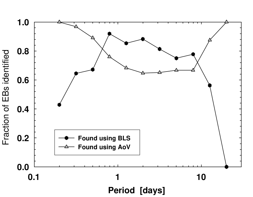
Figure 1: The fraction of the EBs in the final catalog found using the BLS algorithm and the AoV algorithm. The number of EBs in each bin is shown in Figure 8. The BLS method excelled at identifying EBs with short-duration eclipses (compared to the orbital period), which predominately occur at periods $>0.75$ days. The AoV method fared better with EBs that have long-duration eclipses, which predominately occur in sub-day periods. The AoV method also does well with EBs with period longer than $10$ days, which may be dominated by giant-giant binaries (Derekas et al., 2007), and so also have broad eclipses. This plot demonstrates the importance of using multiple independent methods of identifying EB, otherwise the results will have a significant selection effect that may bias any statistical results.

The AoV algorithm is most effective in identifying the periods of LCs with long duration features, such as semi-detached EBs and pulsating stars. The BLS algorithm, in contrast, is effective at identifying periodic systems whose features span only a brief portion of the period, such as detached EBs and transiting planets (see Figure 1). However, the BLS algorithm is easily fooled by outlier data points, identifying them as short duration features. For this reason the BLS algorithm has a significantly higher rate of false positives than AoV, especially for long periods, which have only a few cycles over the duration of the observations. Therefore we limit the search range of the BLS algorithm to periods shorter than 12 days, although as Figure 1 illustrates, its efficiency at locating EBs rapidly declines at periods greater than 10 days.

In step (2), we address the ambiguity between EBs with identical components in a circular orbit, and EBs with extremely disparate components. The phased LC of EBs with identical components contains two identical eclipses, whereas the phased LC of EBs with disparate components will have a secondary eclipse below the photometric noise level. These two cases are degenerate, since doubling the period of a disparate system will result in a LC that looks like an equal-component system. In the pipeline, we handle this problem by doubling such entries; one with the period found in step (1), and another with twice that period. Both of these entries proceed through the pipeline independently. In many cases, after additional processing by the following steps, one of these entries will emerge as being far less likely than the other (see appendix A), at which point it is removed. But in cases where photometry alone cannot determine which is correct, one needs to perform spectroscopic follow up to break the ambiguity. In particular, a double-lined spectrum would support the equal-component hypothesis.

Step (3) is performed using DEBiL, which fits the fractional radii ($r_{1,2}$) and observed magnitudes ($mag_{1,2}$) of the EB’s stellar components, their orbital inclination ($i$) and eccentricity ($e$), and their epoch ($t_{0}$) and argument of periastron ($\omega$). DEBiL first produces an initial guess for these parameters, and then iteratively improves the fit using the downhill simplex method (Nelder, 1965) with simulated annealing (Kirkpatrick et al., 1983; Press et al., 1992).

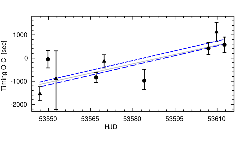
Figure 2: An eclipse timing plot produced in step (4), showing the $O-C$ residuals of the primary eclipses (circles) and the secondary eclipses (triangles). Here, T-Lyr1-14962 is shown with an assumed period of $5.710660\>days$, as measured with an AoV periodogram. The slope of the residuals indicates that the assumed period is inaccurate. The grey solid line is predicted by the best circular-orbit model, whereas the dashed lines are predicted by the best eccentric-orbit model (compare to Figure 3). After correction, we get a fine-tuned period of $5.712516\>days$. This 0.03% correction is small but significant in that without having had this correction, the eclipses would have smeared out and widened.

In step (4), we fine-tune the period ($P$) using a method based on eclipse timing, which we describe below. In order to produce an accurate EB model in step (9) it is necessary to know the system’s period with greater accuracy than that produced in step (1). If we neglect to fine-tune the period, the eclipses may be out of phase with respect to one another, and so the phased eclipses will appear broadened. Our timing method employs the DEBiL model produced in step (3), and uses it to find the difference between the observed and calculated ($O-C$) eclipse epochs. This is done by minimizing the chi-squared fit of the model to the data points in each eclipse, while varying only the model’s epoch of periastron. When the period estimate is off by a small quantity ($\Delta P$), the $O-C$ difference increases by $\Delta P$ each period. This change in the $O-C$ over time can be measured from the slope of the linear regression, which is expected to equal $\Delta P/P$. Thus measuring such an $O-C$ slope will yield the desired period correction (see Figure 2).

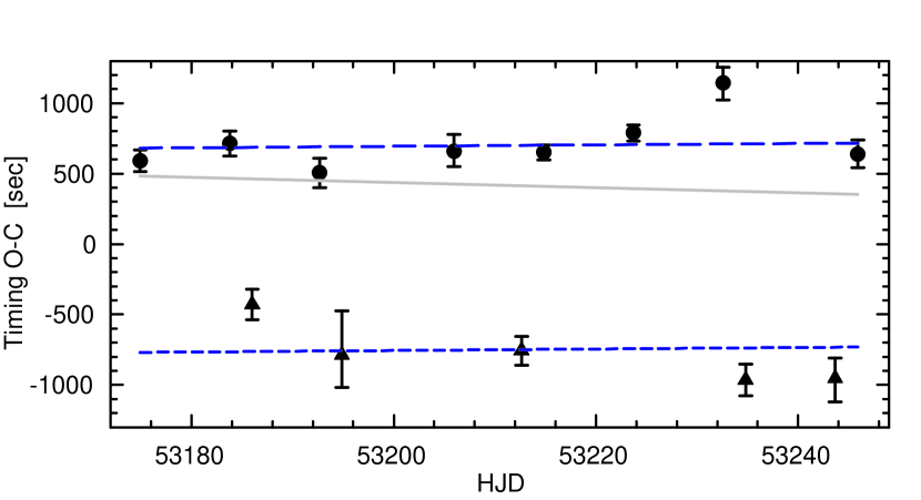
Figure 3: An eclipse timing plot for T-Cyg1-01373, with an assumed period of $4.436013\>days$. In contrast to Figure 2, the slope here is consistent with zero, thus indicating that the period does not need to be fine-tuned. However, the $O-C$ offset between the primary (circles) and secondary (triangle) eclipses is significant ($1449\>seconds$), indicating that this EB has an eccentric orbit. The reduced chi-squared of the best circular-orbit model (grey solid line) is $\chi^{2}_{\nu}=12.9$, while the reduced chi-squared of the best eccentric-orbit model (dashed lines) is $\chi^{2}_{\nu}=0.95$. Applying the $O-C$ timing offset to equation 1 provides a lower limit to the binary’s orbital eccentricity: $e\geq|e\cos\omega|\simeq 0.00594$.

If the EB has an eccentric orbit, the primary and secondary eclipse will separate on the $O-C$ plot, and form two parallel lines with a vertical offset of $\Delta t$ (see Figure 3). We measure this offset and use it as a sensitive method to detect orbital eccentricities. In particular, the value of $\Delta t$ constrains $e\cos\omega$, which in turn provides a lower limit for the system’s eccentricity (Tsesevich, 1973):

$$e\cos\omega\simeq\frac{\pi}{2}\frac{\Delta t}{P}$$ (1)

This formula assumes an orbital inclination of $i=90^{\circ}$, making it a good approximation for eclipsing binaries. We use this method, in combination with DEBiL, to identify the eccentric EBs in the catalog (see Table 3). However, in cases where the eclipse timing measures $|e\cos\omega|<0.005$, or when the eccentricity is consistent with zero, we assume that the EB is non-eccentric, and model it using a circular orbit. We further discuss the physics of these systems in §3.2.

Step (5) is identical to step (3), except that it uses the revised period from step (4). This step provides an improved fit to the LCs, as evidenced by an improved chi-squared value in over 70% of the cases.

In step (6) we locate and remove non-EB sources that seem to be periodic due to photometric contamination by true EBs. Such contaminations result from overlapping point spread functions (PSF) that cause each source to partially blend into the other. These cases can be easily identified with a program that scans through pairs of targets, and selects the ones that both have similar periods (see description below) and are separated by an angle that is smaller than twice the PSF. We found 14 such pairs, all of which were separated by less than $41"$, which is well within twice the TrES PSF ($60"$), while the remaining pairs with similar periods were separated by over $450"$. Upon inspection, all 14 of the pairs we found had similar eclipse shapes, indicating that we had no false positives. Among each pair, we identify the LC with shallower eclipses (in magnitudes) as being contaminated and remove it from the catalog.

We define periods as being similar if the difference between them is smaller than their combined uncertainty. We estimate the period uncertainty using the relation: $\varepsilon_{P}\propto P^{2}/T$, where $T$ is the time interval between the initial and the final observations. One arrives at this relation by noticing that when phasing the LC, the effect of any perturbation from the true period will grow linearly with the number of periods in the LC (see step 4). This amplified effect will become evident once it reaches some fraction of the period itself, in other words, when $\varepsilon_{P}(T/P)\propto P$. A typical TrES LC with a revised period will have a proportionality constant of approximately $1/1000$. In order to avoid missing contaminated pairs (false negatives) we adopt in this step, the extremely liberal proportionality constant of unity.

In step (7) we conduct a visual inspection of all the LC fits. Most EBs were successfully modeled and were included into the catalog as is. About $1\%$ of the LCs analyzed had misidentified periods, as a result of failures of the period finding method of step (1). In most of these cases the period finder indicated either a harmonic of the true period or a rational multiple of a solar or sidereal day. In such cases we use an interactive periodogram to find the correct period and then reprocess the LCs through the pipeline. Some entries were misidentified at step (2) as being ambiguous, even though they have a detectable secondary eclipse or have slightly unequal eclipses. In these cases the erroneous doubled entry was removed. Lastly, some of the EBs were not fit sufficiently well with DEBiL in step (5). These cases were typically due to clustered outlier data points, systematic noise, or severe activity of a stellar component (e.g. flares or spots), which caused DEBiL to produce erroneous initial model parameters. These cases were typically handled by having DEBiL produce the initial model parameters from a more smoothed version of the LC.

In step (8) we match each system, through its coordinates, with the corresponding source in the Two Micron All Sky Survey catalog [2MASS ; (Skrutskie et al., 2006)]. This was done to obtain both accurate target positions and observational magnitudes. These magnitude measurements are then used to derive the colors of each EB, which are incorporated into the MECI analysis, as well as to estimate the EB’s distance modulus (step 9). To this end, 2MASS provides a unique combination of high astrometric accuracy ($\sim$0.1”) together with high photometric accuracy ($\sim$0.015 mag) at multiple near-infrared bands, all while maintaining a decent photometric resolving power ($\sim$3”). By employing these near-infrared bands we both inherently reduce the detrimental effects of stellar reddening, and are able to correct for much of the remaining extinction by fitting for the Galactic interstellar absorbtion.

In order to use the measurements from the 2MASS custom $J$, $H$, and $K_{s}$ filters, we converted them to the equivalent ESO-filter values so that they could be compared to the isochrone table values used in the MECI analysis. This conversion was done using approximate linear transformations (Carpenter, 2001). However, the colors of three EBs (T-And0-10336, T-Cyg1-02304, and T-Per1-05205) were so anomalous that they did not permit a reasonable model solution, thus we chose not to include any color information in their MECI analyses.

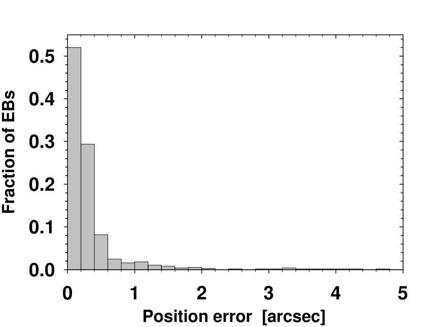
Figure 4: The distribution of the catalog position errors when matching targets to the proper motion databases. In some cases, the position errors are dominated by the motion of the EB during the intervening years.

In addition to its brightness, we also look up each EB’s proper motion. Although proper motion is not required for any of the pipeline analyses, it provides a useful verification for low-mass candidates (see §3.1). These systems are expected to have large proper motions, since they must be nearby to be observable in this magnitude-limited survey. The most extreme such case in the catalog is CM Draconis (T-Dra0-01363), which has a proper motion of over 1300 mas/yr (Salim & Gould, 2003), and is probably the lowest mass system in our catalog. To this end, we match each system to the Second U.S. Naval Observatory CCD Astrograph Catalog [UCAC release 2.4 ; Zacharias et al. (2004)]. When there was no match with UCAC, we use the more comprehensive but less accurate U.S. Naval Observatory photographic sky survey [USNO-B release 1.0 ; Monet et al. (2003)]. These matches were made using the more accurate aforementioned adopted 2MASS coordinates. However, because of their increased observational depth, and the fact that some high-proper motion targets are expected to have moved multiple arcseconds in the intervening decades, we chose to match each target to the brightest ($R$-band) source within 7.5”. It should be noted that the position of CM Draconis shifted by more than 22” and had to be matched manually, though 90% of the matches were separated by less than 0.6”, and 98% were separated by less than 2” (see Figure 4).

The proper motions garnered from these databases can be combined with distance estimates ($D$), to calculate the absolute transverse velocity ($v_{tr}$) of a given EB:

$$v_{tr}\simeq 4.741\>km/sec\left(\frac{PM}{1\>mas/yr}\right)\left(\frac{D}{1\>kpc}\right),$$ (2)

where $PM$ is the system’s angular proper motion. In the catalog we list the right ascension and declination components ($PM_{\alpha}$ and $PM_{\delta}$, respectively), so as to allow one to compute the system’s direction of motion in the sky. The value of $PM$ can be computed from its components, using: $PM^{2}=PM_{\delta}^{2}+PM_{\alpha}^{2}\cos^{2}\delta$, where $\delta$ is the system’s declination. When applying this formula, one should be aware that USNO-B folds the $\cos\delta$ coefficient into its listed $PM_{\alpha}$, while UCAC does not.

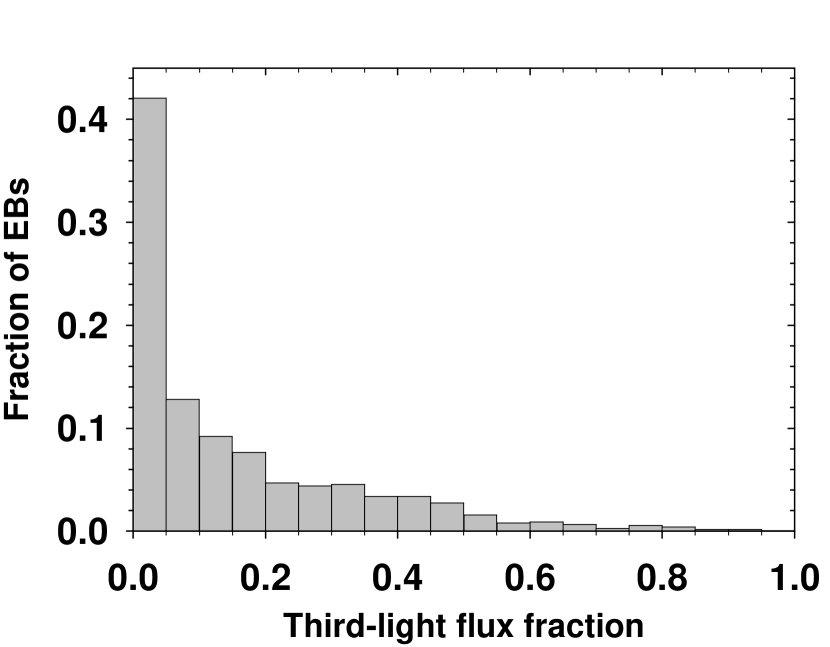
Figure 5: The distribution of the $R$-band third-light flux fraction in the catalog LCs. This fraction was calculated by summing the fluxes of all the USNO-B sources within 30” of the target, excluding the target, and dividing this value by the total flux within 30”, including the target. The resulting fraction ranges from 0 to 1.

Finally, we incorporate the USNO-B photometric $B$- and $R$-magnitude measurements into our catalog to provide a rough estimate of the optical brightness of each target. USNO-B lists two independent measurements in each of these filter, however in some cases one or both of these measurements failed. When both measurements are available, we average them for improved accuracy. However, each measurement has a large photometric uncertainty of $\sim$0.3 mag, thus even these averaged values will have errors that are over an order of magnitude larger that the photometric measurements of 2MASS. For this reason, and because of the increased effect of stellar reddening, we chose not to incorporate these data into the MECI analysis. However, USNO-B’s high photometric resolution ($\sim$1”) enabled us to detect many sources that blended with our targets in the TrES exposures. By summing the $R$-band fluxes of all the USNO-B sources within 30” of each target, we estimated the fraction of third-light included in each LC (see Figure 5). Note that this measure provides only a lower bound to the true third-light fraction, as some EBs are expected to have additional close hierarchical components that would not be resolved by USNO-B. For most of the catalog targets, the third-light flux fraction was found to be small ($<$10%). We therefore conclude that stellar blending will usually have only a minor effect on the MECI analysis results, however users should be aware of the potential biases in the calculated properties of highly blended targets. Though it was not applied to this catalog, in principal, given a third-light flux fraction at a well-determined LC phase, one could correct for the effects of blending.

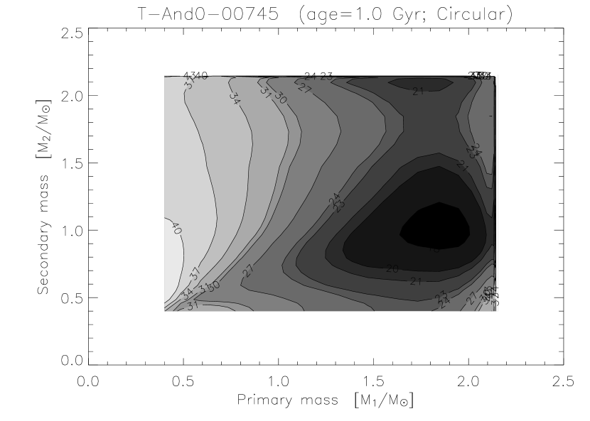
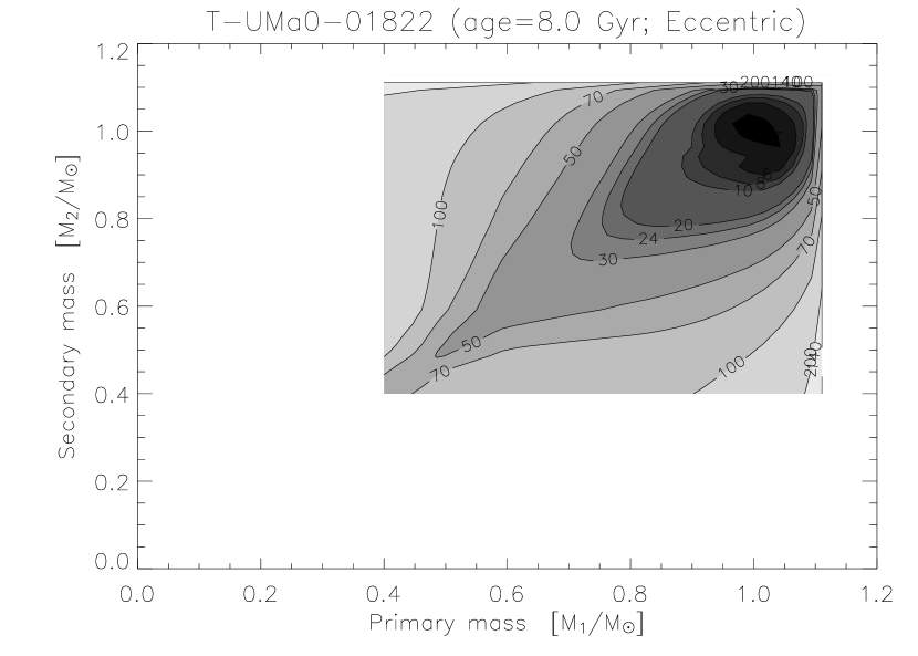
Figure 6: MECI likelihood contour plots of a typical circular-orbit EB (T-And0-00745 ; left) and eccentric-orbit EB (T-UMa0-01822 ; right). There is no significant difference in the way MECI handles these cases, and both usually have a single contour minimum. The plots shown here have the ages set to the values that produced the lowest MECI minima.

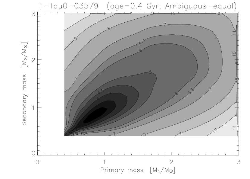
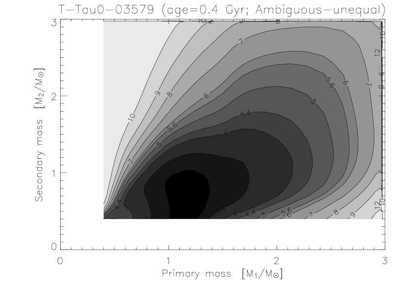
Figure 7: MECI likelihood contour plots of a typical ambiguous EB (T-Tau0-03579). These plots show the effect of assuming that the binary components are equal (left) or unequal (right). Note that the equal-component solution will have a nearly symmetric contour around the diagonal, while the unequal-component solution can provide only an upper limit to the secondary component’s mass, in this case $M_{2}\lesssim 1\>M_{\sun}$. The plots shown here have the ages set to the values that produced the lowest MECI minima.

In step (9) we analyze the LCs with MECI. We refer the reader to the full description of this method in Devor & Charbonneau (2006a, b), and provide here only a brief outline. Given an observed EB LC and out-of-eclipse colors, MECI will iterate through a range of values for the EB age and the masses of its two components. By looking up their radii and luminosities in theoretical isochrone tables, MECI simulates the expected LC and combined colors, and selects the model that best matches the observations, as measured by the chi-squared statistic. Or more concisely, MECI searches the ($M_{1},M_{2},age$)-parameter space for the chi-squared global minimum of each EB. Figures 6 and 7 show constant-age slices through such a parameter space. Once found, the curvature of the global minimum along the parameter space axes is used to determine the uncertainties of the corresponding parameters.

The MECI analysis makes two important assumptions. The first is that EB stellar components are coeval, which has been shown to generally hold for close binaries (Claret & Willems, 2002). When this assumption is violated, MECI will often not be able to find an EB model that successfully reproduces the LC eclipses. Such systems, which may be of interest in their own right, make up $\sim$3% of the catalog and are further discussed later in this section. The second assumption is that there is no significant reddening, or third-light blended into the observations (i.e. from a photometric binary or hierarchical triple). Such blending in the LC will make the eclipses shallower, which produces an effect very similar to that of the EB having a grazing orbit. Thus, it will cause the measured orbital inclination to be erroneous, although it should rarely otherwise affect the results of the MECI analysis significantly. However, the MECI analysis is sensitive to color biases caused by stellar reddening and blending.

We reduce both these biases by incorporating 2MASS colors (see step 8), which are both less suspectable to reddening than optical colors, and suffers from significantly less blending than TrES, as the radius of the 2MASS photometric aperture is $\sim$20 times smaller that that of TrES. We then attempt to further mitigate this problem by analyzing each EB twice, using different relative LC/color information weighting values [see Devor & Charbonneau (2006b) for further details]. We first run MECI with the default weighting value ($w=10$), and then run MECI again with an increased LC weighting ($w=100$) thereby decreasing the relative color weighting. Finally, we adopt the solution that has a smaller reduced chi-square. Typically, the results of the two MECI analyses are very similar, indicating that the observed colors are consistent with the ones predicted by the theoretical isochrones. In such cases, the color information provides an important constraint, which significantly reduces the parameter uncertainties. However, when there is a significant color bias, the default model will not fit the observed data as well as the model that uses a reduced weighting of the color information. In such a case, the reduced color information model, which has a smaller chi-squared, is adopted. Following this procedure, we find that in $\sim$9% of our EBs, the reduced color information model provided a better fit, indicating that while significant color-bias is uncommon, it is a source of error that should not be ignored.

By default, we had MECI use the Yonsei-Yale (Yi et al., 2001; Kim et al., 2002) isochrone tables of solar metallicity stars. Although they successfully describe stars in a wide range of masses, these tables become increasingly inaccurate for low-mass stars, as the stars become increasingly convective. For this reason we re-analyze EBs for which both components were found to have masses below $0.75M_{\sun}$, using instead the Baraffe et al. (1998) isochrone tables, assuming a convective mixing length equal to the pressure scale height. Our EB models also take into account the effects of the limb darkening of each of the stellar components. To this end we employ the ATLAS (Kurucz, 1992) and PHOENIX (Claret, 1998, 2000) tables of quadratic limb-darkening coefficients.

As previously mentioned, once we know the absolute properties of an EB system, we are able to estimate its distance (Stebbing, 1910; Paczynski, 1997), and thus such systems can be considered standard candles. We use Cox (2000) for the extinction coefficients, assuming the standard Galactic ISM optical parameter, $R_{V}=3.1$, to create the following system:

$$mag_{J}-Mag_{J} = \Delta Mag+0.282\cdot A(V)$$ (3)

$$mag_{H}-Mag_{H} = \Delta Mag+0.176\cdot A(V)$$ (4)

$$mag_{K}-Mag_{K} = \Delta Mag+0.108\cdot A(V)$$ (5)

Where $\Delta Mag$ is the extinction-corrected distance modulus, and $A(V)$ is the V-mag absorption due to Galactic interstellar extinction. The estimated distance can then be solved using: $D=10pc\cdot 10^{\Delta Mag/5}$. Because we have three equations for only two unknowns, we adopt the solution that minimizes the sum of the squares of the residuals. In some cases we remove one of the bands as being an outlier (i.e. if it would have resulted in a negative absorption), after which we are still able to solve the systems. But in cases where we need to remove two bands, we set $A(V)=0$ in order to solve for the distance modulus. Although this method has a typical uncertainty of 10% to 20%, it can be applied to EBs that are far more distant and dim than are accessible in other methods, such as parallax measurement. It can be used to map broad features of the Galaxy, and identify binaries that are in the Galactic halo. This method can also be used on large group of systems, so that if the EBs are clustered, one can average their distances, and thus reduce the cluster distance uncertainty as the inverse square root of the number of systems.

In step (10) we perform a final quality check for the EB model fits, and classify them into 7 groups:

1. Eccentric: EBs with unequally-spaced eclipses

2. Circular: EBs with equally-spaced but distinct eclipses

3. Ambiguous-unequal: EBs with undetected secondary eclipses

4. Ambiguous-equal: EB with equally-spaced and indistinguishable eclipses

5. Inverted: detached EBs that are not successfully modeled by MECI

6. Roche-lobe-filling: non-detached EBs that are filling at least one Roche-lobe

7. Abnormal: EBs with atypical out-of-eclipse distortions

We list the model parameters for the EBs of groups I-IV in the electronic version of this catalog (see full description in appendix B). The EBs of groups V-VII could not be well modeled by MECI, therefore we list only their coordinates and periods, so that they can be followed-up.

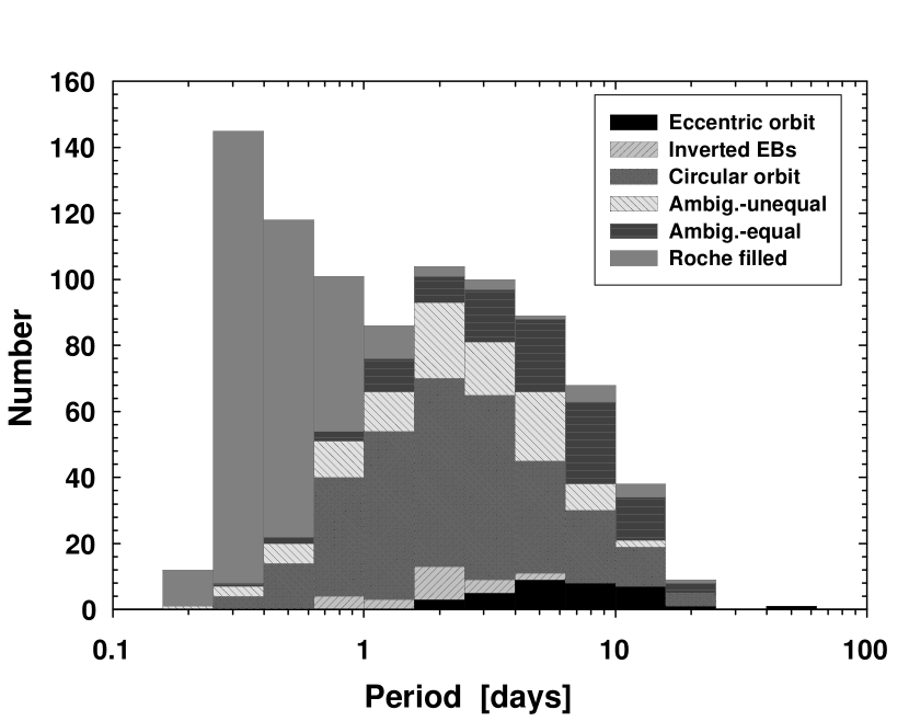
Figure 8: The EB orbital period distribution within the catalog. Each bin is subdivided to show the number of binaries belonging to each of the classification groups described in §2. Note that the ambiguous-equal and ambiguous-unequal entries represent the same stars, with entries in the former group having double the period of the latter. Notice also how the Roche-lobe-filling EBs dominate the sub-day bins, and have a long tail stretching well above 10-day periods. Furthermore, the circular orbit EBs have a period distribution peak of at $\sim$2 days, while the eccentric orbit EBs peak at $\sim$5 days. This is likely due to the orbital circularization that occurs preferentially in short-period systems (see also Figures 22 and 23).

Figure 8 illustrates the period distribution of these seven groups. Note however that both the orbital geometry of EBs (eclipse probability $\propto P^{-2/3}$), and the limited duration of the TrES survey data ($\leq 90\>days$ ; varies from field to field ; see Table 1), act to suppress the detection of binaries with longer periods. An added complication for single-telescope surveys is that about half of the EBs with periods close to an integer number of days will not be detectable, as they eclipse only during the daytime. This EB distribution is consistent with the far deeper OGLE II field catalog (Devor, 2005), where the long tail of Roche-lobe-filling systems has recently been explained by Derekas et al. (2007) as being the result of a strong selection towards detecting eclipsing giant stars.

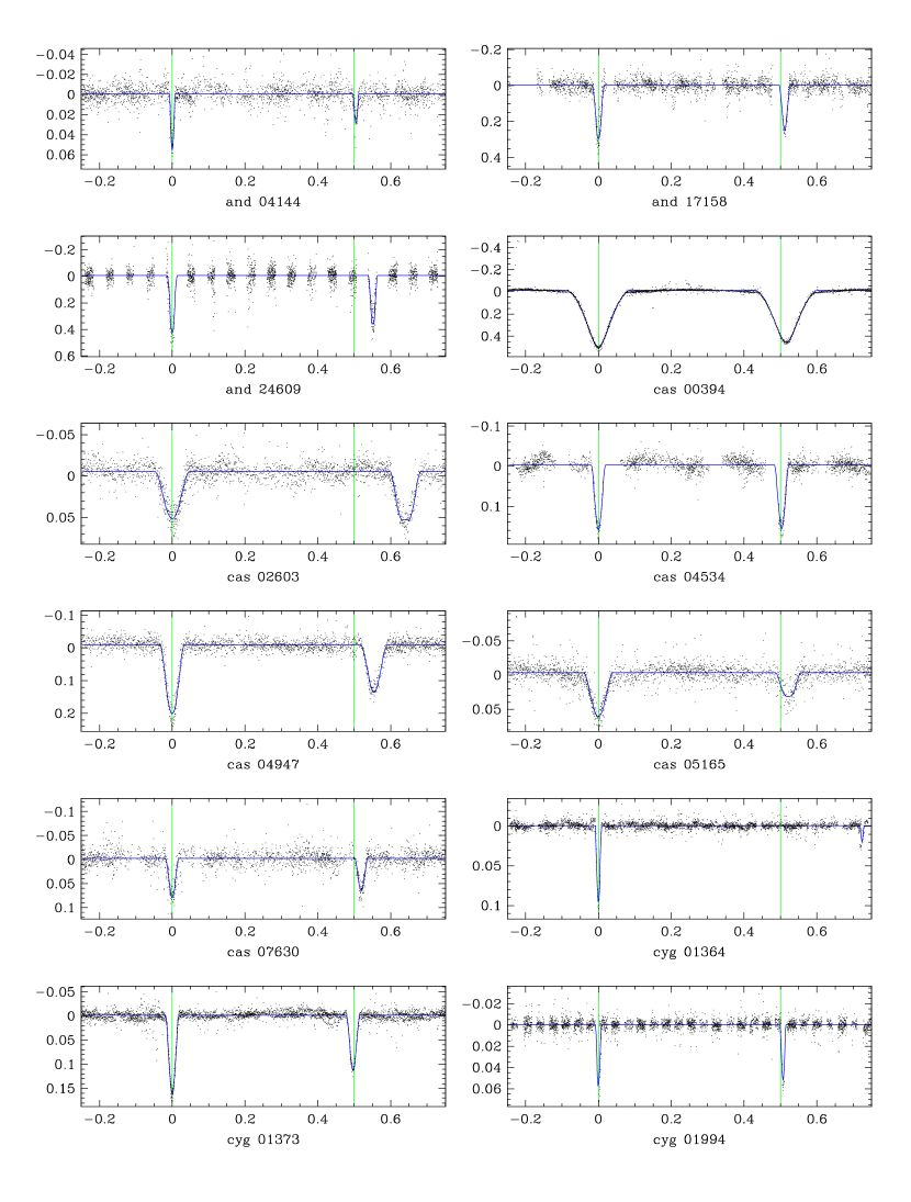
Figure 9: Eccentric EBs (panel 1). Note how the secondary eclipse is not at phase 0.5, as would be in circular orbit EBs.

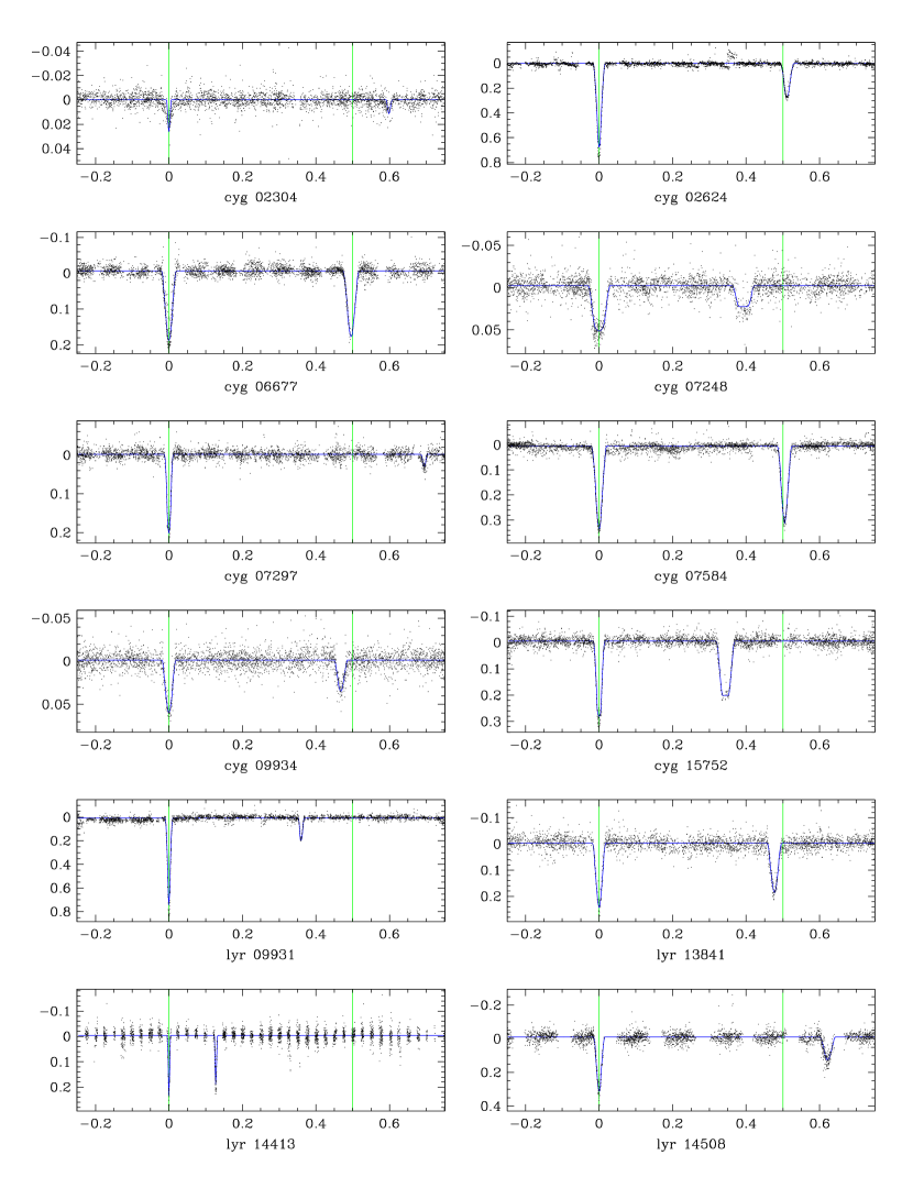
Figure 10: Eccentric EBs (panel 2).

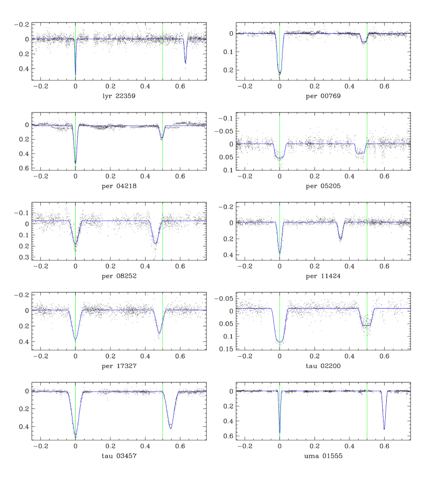
Figure 11: Eccentric EBs (panel 3).

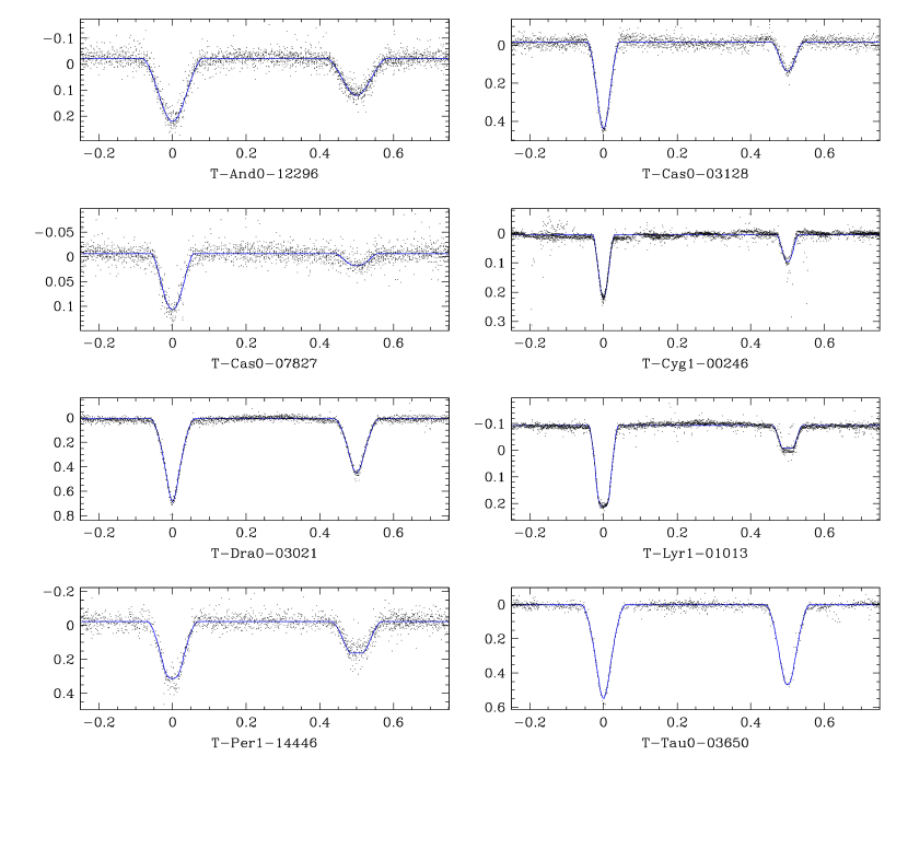
Figure 12: Examples of unambiguous EBs with circular orbits, with their best-fit MECI models (solid line).

Group [I] contains the eccentric EBs identified in step (4) as having centers of eclipse that are separated by a duration significantly different from half an orbital period (see Figures 9, 10, and 11). This criterion is sufficient for demonstrating eccentricity, but not necessary, since we miss systems for which $\cos\omega\simeq 0$ (see equation 1). Fortunately, we are able to detect eccentricities in well-detached EBs with $|e\cos\omega|\geq 0.005$, using eclipse timing. Therefore, assuming that $\omega$ is uniformly distributed, we are approximately 67% complete for $e=0.01$, and over 92% complete for $e=0.04$. In principle, it would be possible to be 100% complete for these systems by measuring the differences in their eclipse durations, however this measurement is known to be unreliable (Etzel, 1991) and so would likely contaminate this group with false positives. Group [II] consists of all such circular-orbit EBs that were successfully fit by a single MECI model (see Figure 12).

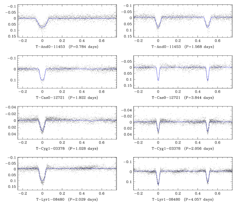
Figure 13: Examples of ambiguous EBs. Left column: assuming very unequal components. Right column: assuming approximately equal components with double the period.

EBs with only one detectable eclipse can potentially be modeled in two alternative ways. One way is to assume very unequal stellar components, which have a very shallow undetected secondary eclipse (group [III]). Since we cannot estimate the eccentricity of such systems, we assume that they have circular orbits. The other way is to assume that the period at hand is twice the correct value, and that the components are nearly equal (group [IV]). The entries of such ambiguous LCs were doubled in step (2), so that these two solutions would be independently processed through the pipeline (see Figure 13). Therefore, these two groups have a one-to-one correspondence between them, although only one entry of each pair can be correct. Resolving this ambiguity may not always be possible without spectroscopic data. In some cases we were able to resolve this ambiguity using either a morphological or a physical approach. The morphological approach consists of manually examining the LCs of group [IV] for any asymmetries in the two eclipses (e.g. width, depth, or shape), or in the two plateaus between the eclipses (e.g. perturbations due to tidal effects, refections, or the “O’Connell effect”). The physical approach consists of applying our understanding of stellar evolution in order to exclude entries that cannot be explained through any coeval star pairing (see appendix A). Either way, once one of the two models has been eliminated, the other model is moved into group [II] and is adopted as a non-ambiguous solution. It is interesting to note that when analyzing the two models with MECI, the equal-component solution (group [IV]) has masses approximately equal to the primary component of the unequal-component solution (group [III]). The mass of the unequal-component solution’s secondary component will typically be the smallest value listed in the isochrone table, as this configuration will produce the least detectable secondary eclipse.

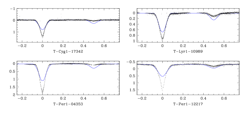
Figure 14: Examples of EBs classified as inverted EBs. We included the unsuccessful best-fit MECI model (solid curve) as an approximate reference to illustrate the LC of a corresponding binary that has had no mass transfer. Notice how the model LC is unable to achieve a sufficiently deep primary eclipse, while producing a secondary eclipse that is too deep.

Group [V] consists of detached EBs that cannot be modeled by two coeval stellar components. As mentioned earlier, we can reject the single-eclipse solution for EBs with sufficiently deep eclipses (see appendix A). This argument can be further extended to cases where we can detect both eclipses in the LC, but where one is far shallower than the other. In some cases, no two coeval main-sequence components will reproduce such a LC, but unlike the previous case, since both eclipses are seen, we cannot conclude that the period needs to be doubled. Such systems are likely to have had mass transfer from a sub-giant component onto a main-sequence component through Roche-lobe overflow, to the point where currently the main-sequence component has become significantly more massive and brighter than it was originally (Crawford, 1955). This process will cause the components to effectively behave as non-coeval stars, even though they have in fact the same chronological age. In extreme cases, the originally lower-mass main-sequence component can become more massive than the sub-giant, and thus swap their original primary/secondary designations, so that the main-sequence component is now the primary component. We call such systems “inverted” EBs, and place them into group [V] (see Figure 14). This phenomenon is often referred to in the literature as the “Algol paradox”, though we chose not to adopt this term so as to avoid confusing it with the term “Algol-type EB” (EA), which is defined by the General Catalogue of Variable Stars [GCVS ; (Kukarkin, 1948; Samus, 2006)] as being the class of all well-detached EBs.

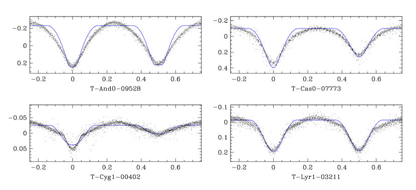
Figure 15: Examples of EBs that are assumed to have filled at least one of their Roche lobes. We included, for illustration purposes only, their best-fit MECI models (solid line). These models were not adopted since they neglect tidal distortions, reflections, and gravity darkening effects, and so produce a poor fit to the data.

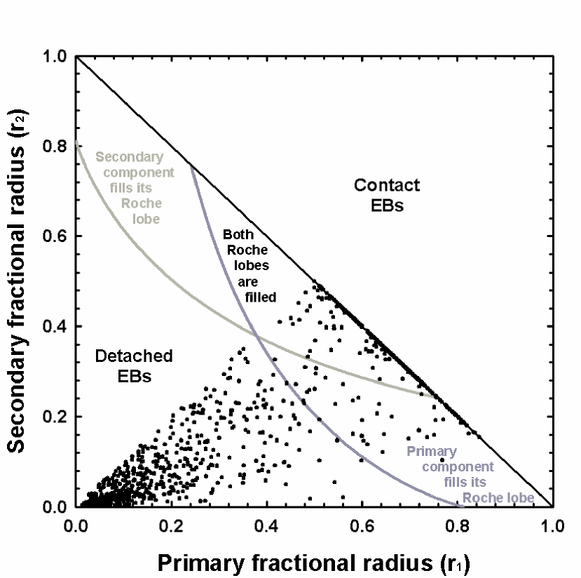
Figure 16: The criterion applied in equations 6 and 7 to determine whether one or both the EB components have filled their Roche lobe, and thus need to be placed into group (6).

Group [VI] contains the EBs that have at least one component filling its Roche-lobe (see Figure 15). Such system cannot be well-fit by either DEBiL or MECI since they assume that the binary components are detached, and so neglect tidal and rotational distortions, gravity darkening, and reflection effects. These systems must be separated from the rest of the catalog since their resulting best-fit models will be poor and therefore their evaluated physical attributes will likely be erroneous. In a similar fashion to Tamuz et al. (2006), we detect these systems automatically by applying the Eggleton (1983) approximation for the Roche-lobe radius, and place in group [VI] all the systems for which at least one of the EB components has filled its Roche-lobe (see Figure 16), that is, if either one of the following two inequalities occurs:

$$r_{1} > \frac{0.49\>q^{-2/3}}{0.6\>q^{-2/3}+\ln\left(1+q^{-1/3}\right)}{\rm\ \ \ or}$$ (6)

$$r_{2} > \frac{0.49\>q^{2/3}}{0.6\>q^{2/3}+\ln\left(1+q^{1/3}\right)}\ ,$$ (7)

where $q=M_{2}/M_{1}$ is the EB components’ mass ratio. Since we expect non-detached EBs to be biased towards evolving, higher mass stellar components, we estimated $q$ using the early-type mass-radius power law relation found in binaries (Gorda & Svechnikov, 1998): $q\simeq(r_{2}/r_{1})^{1.534}$. Although in principle, we could have estimated $q$ directly from the EB component masses resulting from the MECI analysis, we chose not to, since as stated above, the analysis of such systems is inaccurate. The analytic approximation we used, though crude, proved to be remarkably robust, as we found only 5 false negatives and no false positives when visually inspecting the LCs. We found many more false positives/negatives when using the alarm criteria suggested by Devor (2005) or Mazeh et al. (2006), both of which attempt to identify bad model fits by evaluating spatial correlations of the model’s residuals.

Finally, group [VII] contains systems visually identified as EBs (i.e. having LCs with periodic flux dips), yet having atypical LC perturbations that indicate the existence of additional physical phenomena (see Figures 17 and 18). For lack of a better descriptor, we call such systems “abnormal” (see further information in §3.3). This group is different from the previous six in that we cannot automate their classification, and their selection is thus inherently subjective. In 15 of the 20 systems, we were able to approximately model the LCs, and included them in one of the aforementioned groups. In these cases users should be aware that these model may be biased by the phenomenon that brought about their LC distortion.

3 Results

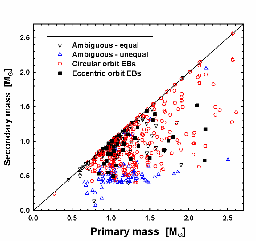
Figure 19: The mass-mass relation for the detached EBs of the TrES dataset. Each category is represented by a different symbol. Note that the ambiguous EBs are plotted twice, where only one of the solution can be correct. Notice also that in the equal-component solutions are clustered along the diagonal, while the unequal-component solutions are clustered along the minimum available mass of the Yonsei-Yale isochrones ($0.4\>M_{\sun}$). Some of the ambiguous solutions deviate from these clusters due to poor constraints on the secondary eclipse, which brings about a large uncertainty. Finally, notice the sparsity of EBs populating the low-mass corner of this plot ($M_{1,2}<0.75\>M_{\sun}$). These systems, whose importance is outlined in §3.1, were modeled using the Baraffe isochrones. CM Draconis (T-Dra0-01363) clearly sets itself apart, being the lowest-mass binary in the catalog (circle at bottom-left).

We identified and classified a total of 773 EBs. These systems consisted of 734 EBs with circular orbits, 34 detached EBs with eccentric orbits (group [I] ; Table 3), and 5 unclassified abnormal EBs (group [VII] ; Table 5). We marked 15 of the detached EBs with circular orbits as also being abnormal. Of the 734 EBs with circular orbits, we classify 290 as unambiguous detached EBs (group [II] ; Table 7), 103 as ambiguous detached EBs, for which we could not determine photometrically if they consisted of equal or disparate components (groups [III] and [IV] ; Table 6), 23 as inverted EBs (group [V] ; Table 8), and 318 as non-detached (group [VI] ; Table 4). With the exception of the abnormal EBs, which were selected by eye, we use an automated method to classify each of these groups (see §2 for details). Our mass estimates for the primary and secondary components are plotted in Figure 19.

The EB discovery yield (the fraction of LCs found to be EBs), varies greatly from field to field, ranging from 0.72% for Cygnus, to 0.15% for Corona Borealis (see Table 2). This variation is strongly correlated with Galactic latitude, where fields near the Galactic plane have larger discovery yields than those that are farther from it (see Figure 20). This effect is likely due to the fact that fields closer to the Galactic plane contain a higher fraction of early-type stars. These early-type stars are both physically larger, making them more likely to be eclipsed, and are more luminous, which has them produce brighter and less noisy LCs, thereby enabling the detection of EBs with shallower eclipses. Furthermore, much of the residual scatter can be attributed to the variation in the observed duration of each field (see Table 1). That is, we find additional EBs, with longer periods, in fields that were observed for a longer duration.

Currently, 88 of the cataloged EBs (11%) appear in either the International Variable Star Index (VSX), or in the SIMBAD astronomical database (Table 9). However, only 49 systems (6%) have been identified as being variable. Not surprisingly, with few exceptions, these targets were among the brightest sources of the catalog. Using only photometry, it is often notoriously difficult to distinguish non-detached EBs from pulsating variables that vary sinusoidally in time, such as type-C RR Lyrae. Furthermore, unevenly spotted stars may also cause false positive identifications, especially in surveys with shorter durations. Ultimately, spectroscopic follow-up will always be necessary to confirm the identification of such variables.

We highlight three groups of EBs as potentially having special importance as test beds for current theory. For more accurate properties, these EBs will likely need to be followed up both photometrically and spectroscopically. The brightness of these EBs will considerably facilitate their follow-up.

3.1 Low-mass EBs

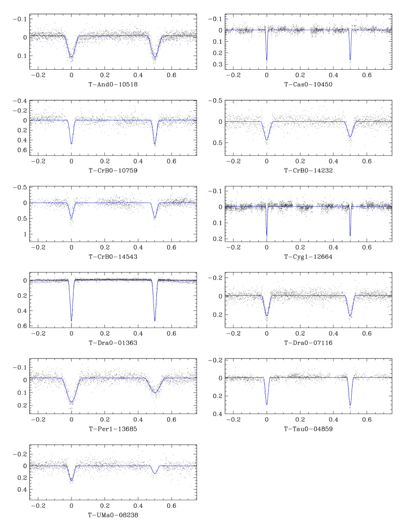
Figure 21: Low mass candidates ($M_{1}<0.75M_{\sun}$), with their best-fit MECI models (solid line).

The first group consists of 11 low-mass EB candidates, including 10 newly discovered EBs with either K or M-dwarf stellar components. Our criteria for selecting these binaries were that they be well-detached, and that both components have estimated masses below $0.75M_{\sun}$ (see Table 10 and Figure 21). Currently, only 7 such detached low-mass EBs have been confirmed [YY Gem (Kron, 1952; Torres & Ribas, 2002), CM Dra (Lacy, 1977b; Metcalfe et al., 1996), CU Cnc (Delfosse et al., 1999; Ribas, 2003), T-Her0-07621 (Creevey et al., 2005), GU Boo (López-Morales & Ribas, 2005), NSVS01031772 (López-Morales et al., 2006), and UNSW-TR-2 (Young et al., 2006)].

Despite a great deal of work that has been done to understand the structure of low-mass stars [e.g. Chabrier & Baraffe (2000)], models continue to underestimate their radii by as much as $15$% (Lacy, 1977a; Torres & Ribas, 2002; Creevey et al., 2005; Ribas, 2006), a significant discrepancy considering that for solar-type stars the agreement with the observations is typically within $1-2$% (Andersen, 1991, 1998). In recent years an intriguing hypothesis has been put forward that strong magnetic fields may have bloated these stars through chromospheric activity (Ribas, 2006; Torres et al., 2006; López-Morales, 2007; Chabrier et al., 2007). Furthermore, Torres et al. (2006) find that such bloating occurs even for stars with nearly a solar mass, and suggest that this effect may also be due to magnetically induced convective disruption. In either case, these radius discrepancies should diminish for widely separated binaries with long periods, as they become non-synchronous and thus rotate slower, which according to dynamo theory would reduce the strength of their magnetic fields.

Unfortunately, the small number of well characterized low-mass EBs makes it difficult to provide strong observational constraints to theory. Despite the fact that such stars make up the majority of the Galactic stellar population, their intrinsic faintness renders them extremely rare objects in magnitude-limited surveys. In addition, once found, their low flux severely limits the ability of observing their spectra with both sufficiently high resolution and a high signal-to-noise ratio. To this end, the fact that the TrES survey was made with small-aperture telescopes is a great advantage, as any low-mass EB candidate found is guaranteed to be bright, and thus require only moderate-aperture telescopes for their follow-up. Thus we propose multi-epoch spectroscopic study of the systems listed here, in order to confirm their low mass and to estimate their physical properties with an accuracy sufficient to test models of stellar structure. Moreover, two of our candidates (T-Cyg1-12664 and T-Cas0-10450), if they are in fact ambiguous-equal (group [IV]), have periods greater than 8 days, making them prime targets for testing the aforementioned magnetic-bloating hypothesis.

3.2 Eccentric EBs

The second group of EBs consists of 34 binaries with eccentric orbits (see Table 3, and Figures 9, 10, and 11). We were able to reliably measure values of $|e\cos\omega|$ as low as $\sim 0.005$ by using the eclipse timing technique (see §2 and Figure 3). Since this measure provides a lower limit to the eccentricity, it is well-suited to identify eccentric EBs, even though the actual value of the eccentricity may be uncertain. As mentioned earlier, in an effort to avoid false-positives, we do not include in this group EBs whose eclipse timing measures $|e\cos\omega|<0.005$, or EBs with an eccentricity consistent with zero.

Our interest in these eccentric binaries stems from their potential to constrain tidal circularization theory (Darwin, 1879). This theory describes how the eccentricity of a binary orbit decays over time due to tidal dissipation, with a characteristic timescale ($t_{circ}$) that is a function of the components’ stellar structure and orbital separation. As long as the components’ stellar structure remains unchanged, the orbital eccentricity is expected to decay approximately exponentially over time [$e\propto\exp(-t/t_{circ})$]. However, once the components evolve off the main sequence, this time scale may vary considerably (Zahn & Bouchet, 1989). Thus, to understand the circularization history of binaries with circularization timescales similar to or larger than their evolutionary timescales, one must integrate over the evolutionary tracks of both stellar components.

Three alternate tidal dissipation mechanisms have been proposed: dynamical tides (Zahn, 1975, 1977), equilibrium tides (Zahn, 1977; Hut, 1981), and hydrodynamics (Tassoul, 1988). Despite its long period of development, the inherent difficulty of observing tidal dissipation has prevented definitive conclusions. Zahn & Bouchet (1989) add a further complication by maintaining that most of the orbital circularization process takes place at the beginning of the Hayashi phase, and that the eccentricity of a binary should then remain nearly constant throughout its lifetime on the main sequence.

Observational tests of these tidal circularization theories, whereby $t_{circ}$ is measured statistically in coeval stellar populations, have so far proved inconclusive. North & Zahn (2003) found that short-period binaries in both the Large and Small Magellanic Clouds seem to have been circularized in agreement with the theory of dynamical tides. However, Meibom & Mathieu (2005) show that with the exception of the Hyades, the stars in the clusters that they observed were considerably more circularized than any of the known dissipation mechanisms would predict. Furthermore, they find with a high degree of certainty, that older clusters are more circularized than younger ones, thereby contradicting the Hayashi phase circularization model.

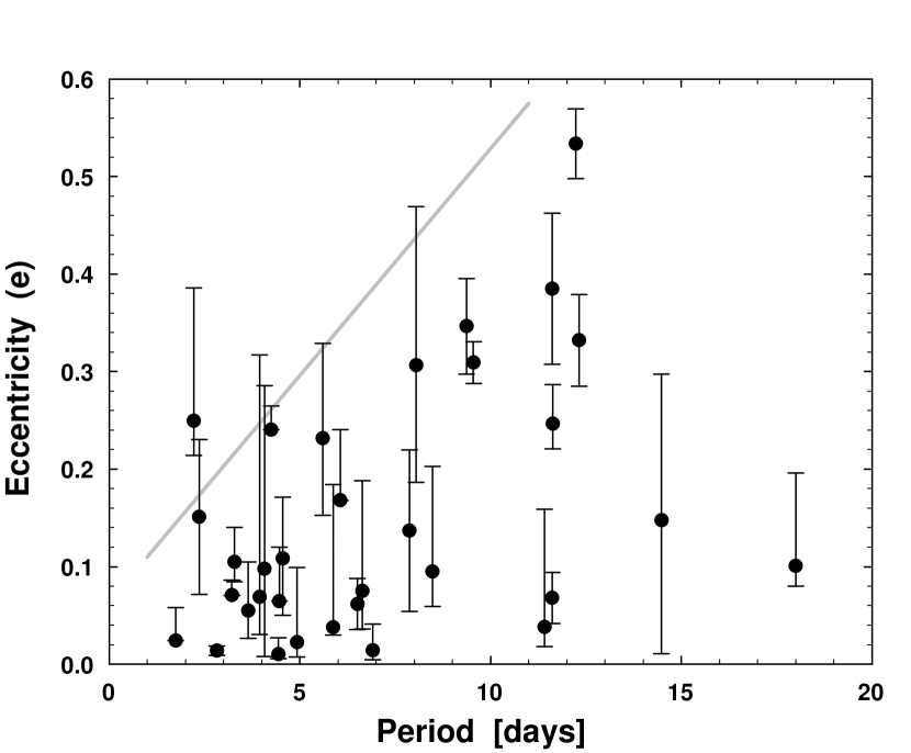
Figure 22: The period-eccentricity relation. The lower end of the error bars were truncated, where needed, by the measured lower limit, $|e\cos\omega|$. Note the lack of eccentric short period systems. The diagonal line is provided to guide the eye.

Encouraged by the statistical effect of circularization that can be seen in our catalog (Figure 22), we further estimated $t_{circ}$ for each of the eccentric systems as follows. Zahn (1977, 1978) provides an estimate for the orbital circularization timescale due to turbulent dissipation in stars possessing a convective envelope, assuming that corotation has been achieved:

$$t_{circ}=\frac{1}{21q(1+q)k_{2}}\left(\frac{MR^{2}}{L}\right)^{1/3}\left(\frac{a}{R}\right)^{8}$$ (8)

where $M,R,L$ are the star’s mass, radius and luminosity, and $k_{2}$ is the apsidal motion constant of the star, which is determined by its internal structure and dynamics.

More massive stars, which do not have a convective envelope but rather develop a radiative envelope, are thought to circularize their orbit using radiative damping (Zahn, 1975; Claret & Cunha, 1997). This is a far slower mechanism, whose circularization timescale can be estimated by:

$$t_{circ}=\frac{2}{21q(1+q)^{11/6}E_{2}}\left(\frac{R^{3}}{GM}\right)^{1/2}\left(\frac{a}{R}\right)^{21/2}$$ (9)

where $E_{2}$ is the tidal torque constant of the star, and $G$ is the universal gravitational constant. We can greatly simplify these expressions by applying Kepler’s law [$a^{3}=GM(1+q)(P/{2\pi})^{2}$], and adopt the Cox (2000) power law approximations for the main-sequence mass-radius and mass-luminosity relations. For the convective envelope case, we adopt the late-type mass-radius relation ($M<1.3M_{\sun}$), and for the radiative envelope case we adopt the early-type mass-radius relation ($M\geq 1.3M_{\sun}$), thus arriving at:

$$t_{circ}\simeq\cases{0.53Myr\;(k_{2}/0.005)^{-1}q^{-1}(1+q)^{5/3}\left(P/day\right)^{16/3}\left(M/M_{\sun}\right)^{-4.99},\ M<1.3M_{\sun}\cr 1370Myr\;(E_{2}/10^{-8})^{-1}q^{-1}(1+q)^{5/3}\left(P/day\right)^{7}\left(M/M_{\sun}\right)^{-2.76},\ M\geq 1.3M_{\sun}\cr}$$ (10)

Determining the value of $k_{2}$ and $E_{2}$ is the most difficult part of this exercise, since their values are a function of the detailed structure and dynamics of the given star, which in turn changes significantly as the star evolves (Claret & Cunha, 1997; Claret & Willems, 2002). In our calculation, we estimate these values by interpolating published theoretical tables [$k_{2}$: Zahn (1994), $E_{2}$: Zahn (1975); Claret & Cunha (1997)]. Since both stellar components contribute to the circularization process, the combined circularization timescale becomes $t_{circ}=1/(t_{circ,1}^{-1}+t_{circ,2}^{-1})$, where the subscripts $1$ and $2$ refer to the primary and secondary binary components (Claret & Cunha, 1997). In Table 3, we list the combined circularization timescale for each of the eccentric EBs we identify.

The value of $t_{circ}$ for most of the eccentric systems (21 of 34) is larger than the Hubble time, indicating that no significant circularization is expected to have taken place since they settled on the main sequence. About a quarter of the eccentric systems (8 of 34) have a $t_{circ}$ smaller than the Hubble time but larger than $1\>Gyr$. While circularization is underway, the fact that they are still eccentric is consistent with theoretical expectations. The remaining systems (5 of 34) all have $t_{circ}<1\>Gyr$, have periods less than 3.3 days, and unless they are extremely young, require an explanation for their eccentric orbits. Two of these EBs (T-Tau0-02487 and T-Tau0-03916) are located near the star forming regions of Taurus, supporting the hypothesis that they are indeed young. However, this hypothesis does not seem to be adequate for T-Cas0-02603, which has a period of only 2.2 days and $t_{circ}\simeq 0.26\>Gyr$, while possessing a large eccentricity of $e\simeq 0.25$. An alternative explanation is that some of these binaries were once further apart, having larger orbital periods, and thus larger circularization timescales. These systems may have been involved in a comparably recent interaction with a third star (a collision or near miss), or have been influenced by repeated resonant perturbations of a tertiary companion.

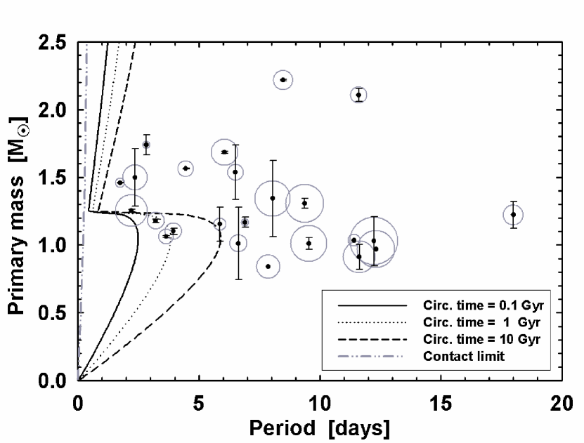
Figure 23: The period-primary mass relation for eccentric EBs. We included all systems with well-determined masses. The area of the grey circles is proportional to the EB’s eccentricity. All the curves are theoretical boundaries, assuming that the binary components are both on the main sequence and have equal masses ($q=1$). The left-most dot-dash line demarcates the binary contact limit, and the remaining curves mark systems with increasing circularization time (see equation 10). Note the abrupt increase in the circularization time for systems more massive than $\sim 1.25M_{\sun}$, at which point the stellar convective envelope becomes radiative, and thus far less efficient at tidal dissipation.

Finally, we would like to draw the reader’s attention to our shortest-period eccentric EB, T-Cas0-00394, whose period is a mere 1.7 days. Notably, this system is entirely consistent with theory, since its mass falls in a precarious gap, where the stellar envelopes of its components are no longer convective, yet their radiative envelopes are not sufficiently extended to produce significant tidal drag (see Figure 23).

3.3 Abnormal EBs

The third group of EBs consists of 20 abnormal systems (see Table 5, and Figures 17 and 18). While possessing the distinctive characteristics of EBs, these LCs stood out during manual inspection for a variety of reasons. These systems underline the difficulty of fully automating any LC pipeline, as any such system will inevitably need to recognize atypical EBs that were not encountered before.

The LCs we listed can be loosely classified into groups according to the way they deviate from a simple EB model. A few cases exhibited pulsation-like fluctuations that were not synchronized with the EB period (shorter-period: T-Dra0-00398, longer-period: T-Lyr1-00359, T-Per1-00750). These fluctuations may be due either to the activity of an EB component, or to a third star whose light is blended with the binary. In principle, one can identify the active star by examining the amplitude of the fluctuations during the eclipses. If the fluctuations originate from one of the components, their observed amplitude will be reduced when the component is being eclipsed. In such a case, if the fluctuations are due to pulsations, they can further provide independent constraints to the stellar properties through astro-seismological models (Mkrtichian et al., 2004). To identify such fluctuating EBs one must subtract the fitted EB model from the LC, and evaluate the residuals [e.g. Pilecki & Szczygiel (2007)]. When the fluctuation period is fixed, one can simply search the residual LC using a periodogram, as was done in step (1) of our pipeline (see §2). However, when the fluctuation period varies (i.e. non-coherent), as in the aforementioned LCs, one must employ alternate methods, since simply phasing their LC will not produce any discernable structure. For LCs with long-period fluctuations one can directly search the residuals for time dependencies, while for LCs with short-period fluctuations one can search the residuals for non-Gaussian distributions. However, in practice these measurements will likely not be robust, as there are many instrumental effects that can produce false positives. Thus, we employ a search for auto-correlations in the residual time series, which overcomes most instrumental effects, while providing a reliable indicator for many types of pseudo-periodic fluctuations.

The remaining systems had LC distortions that appear to be synchronized with the orbital period. The source of these fluctuations is likely due to long-lasting surface inhomogeneities on one or both of the rotationally synchronized components. When the LC has brief periodic episodes of darkening (T-And0-11476, T-Cas0-13944, T-Cyg1-07584, T-Dra0-04520), they can usually be explained as stable star spots, but brief periodic episodes of brightening (T-And0-04594, T-Her0-08091), which may indicate the presence of stable hot-spots, are more difficult to interpret. This phenomenon is especially puzzling in the aforementioned two cases, in which the brightening episodes are briefer than one would expect from a persistent surface feature and repeat at the middle of both plateaus.

When the two plateaus of a LC are not flat, they are usually symmetric about the center of the eclipses. This is due to the physical mirror symmetry about the line intersecting the binary components’ centers. When the axis of symmetry does not coincide with the center of eclipse (T-And0-00920, T-Cyg1-08866, T-Dra0-03105, T-Lyr1-07584, T-Lyr1-15595), a phenomenon we term “eclipse offset”, we conclude that this symmetry must somehow be broken. This may occur if the EB components are not rotationally synchronized, or have a substantial tidal lag. Another form of this asymmetry can appear as an amplitude difference between the two LC plateaus (T-Her0-03497, T-Lyr1-13166, T-Per1-08789, T-UMa0-03090). This phenomenon, which was originally called the “periastron effect” and has since been renamed the “O’Connell effect”, has been known for over a century, and has been extensively studied [e.g. O’Connell (1951); Milone (1986)]. Classic hypotheses suggest an uneven distribution of circumstellar material orbiting with the binary (Struve, 1948) or surrounding the stars (Mergentaler, 1950), either of which could induce a preferential $H^{-}$ absorption on one side. Binnendijk (1960) was the first of many to suggested that the this asymmetry is due to subluminous regions of the stellar surface (i.e. star spots). However, this explanation also requires the stars to be rotationally synchronized, and for the spots to be stable over the duration of the observations. Alternate models abound, including a hot spot on one side of a component brought about through mass transfer from the other component, persistent star spots created by an off-axis magnetic field, and circumstellar material being captured by the components and heating one side of both stars (Liu & Yang, 2003). As with many phenomena that have multiple possible models, the true answer may involve a combination of a number of these mechanisms, and will likely vary from system to system (Davidge & Milone, 1984).

Finally, a few particularly unusual LCs (T-Dra0-03105, T-Lyr1-05984) display a very large difference between their eclipse durations. Although a moderate difference could be explained by an eccentric orbit, such extreme eccentricities in systems with such short orbital periods (0.5 and 1.5 days) are highly unlikely.

4 Conclusions

We presented a catalog of 773 eclipsing binaries found in 10 fields of the TrES survey, identified and analyzed using an automated pipeline. We described the pipeline we used to identify and model them. The pipeline was designed to be mostly automated, with manual inspections taking place only once the vast majority of non-EB LCs had been automatically filtered out. At the final stage of the pipeline we classified the EBs into 7 groups: eccentric, circular, ambiguous-equal, ambiguous-unequal, inverted, Roche-lobe-filling, and abnormal. The former four groups were all successfully modeled with our model fitting program. However, the latter three groups possessed significant additional physical phenomena (tidal distortions, mass-transfer, and surface activity), which did not conform to the simple detached-EB model we employed.

We highlighted three groups of binaries, which may be of particular interest and warrant follow-up observations. These groups are: low-mass EBs, EBs with eccentric orbits, and abnormal EBs. The low-mass EBs (both components $<0.75M_{\sun}$) allow one to probe the mass-radius relation at the bottom of the main-sequence. Only 7 such EBs have previously been confirmed, and the physical properties of many of them are inconsistent with current theoretical models. Our group of 10 new candidates will likely provide considerable additional constraints to the models, and the discovery of 2 long period systems could help confirm a recent hypothesis that this inconsistency is due to stellar magnetic activity. The eccentric-orbit EBs may help confirm and constrain tidal circularization theory, as many of them have comparably short circularization timescales. We demonstrated that, as one would predict from the theory, the shortest period systems fall within a narrow range of masses, in which their stellar envelopes cease to be convective yet their envelopes are not extended enough to produce significant tidal drag. The abnormal EBs seem to show a plethora of effects that are indicative of asymmetries, stellar activity, persistent hot and cold spots, and a host of other physical phenomena. Some of these systems may require dedicated study to be properly understood.

In the future, as LC datasets continue to grow, it will become increasingly necessary to use such automated pipelines to identify rare and interesting targets. Such systematic searches promise a wealth of data that can be used to test and constrain theories in regions of their parameter-space that were previously inaccessible. Furthermore, even once the physics of “vanilla” systems has been solved, more complex cases will emerge to challenge us to achieve a better understanding of how stars form, evolve and interact.

Appendix A Rejecting single-eclipse EB Models

An EB LC comprised of a deep eclipse and a very shallow eclipse, can occur in one of two ways. Either the secondary component is luminous but extremely small (e.g. a white dwarf observed in UV), thus producing a shallow primary eclipse, or the secondary component is comparably large but extremely dim, thus producing a shallow secondary eclipse. The first case, though possible [e.g. Maxted et al. (2004)], is extremely rare, and will have a signature “flat bottom” to the eclipse. We have not encountered such a LC in our dataset. The second case will have a rounded eclipse bottom, due to the primary component’s limb darkening. Assuming this latter contingency, in which the secondary component is dark in comparison to the primary component, we can place a lower bound to its radius ($R_{2}$):

$$R_{2}\geq R_{1}\sqrt{1-10^{-0.4\Delta mag_{1}}}\ ,$$ (A1)

where $R_{1}$ is the radius of the primary component, and $\Delta mag_{1}$ is the magnitude depth of the primary eclipse. Thus, if the eclipse is very deep, the size of the secondary component must approach the size of the primary component. However, coeval short-period detached EBs with components of similar sizes yet desperate luminosities are expected to be very rare, assuming they follow normal stelar evolution. Therefore, if only one eclipse is detected, and it is both rounded and sufficiently deep, we may conclude that this configuration entry is likely to be incorrect, and that the correct configuration has double the orbital period and produces two equal eclipses. Only when we cannot apply such a period doubling solution (i.e. when the secondary eclipse is detectable), do we resort to questioning our assumption of normal stelar evolution (see classification group V, described in §2).

Appendix B Description of the Catalog Fields

Due to the large size of the catalog we were only able to list small excerpts of it in the body of this paper. Readers interested in viewing the catalog in its entirety can download it electronically. Note that although the catalog lists 773 unique systems, each of the 103 ambiguous EBs appear in both possible configurations (see §2), raising the total number of catalog entries to 876. Below, we briefly describe the catalog’s 38 columns. The column units, if any, are listed in square brackets.

1. $Category$ - the EB’s classification (see §2).

2. $Binary\ name$ - the EB’s designation, which is composed of its TrES field (see Table 1) and index.

3. $\alpha$ - the EB’s right ascension (J2000).

4. $\delta$ - the EB’s declination (J2000).

5. $Period$ [days] - the EB’s orbital period.

6. $Period\ uncertainty$ [days] - the uncertainty in the EB’s orbital period.

7. $Mass_{1}$ [$M_{\sun}$] - the mass of the EB’s primary (more massive) component.

8. $Mass_{1}\ uncertainty$ [$M_{\sun}$] - the uncertainty in the primary component’s mass.

9. $Mass_{2}$ [$M_{\sun}$] - the mass of the EB’s secondary (less massive) component.

10. $Mass_{2}\ uncertainty$ [$M_{\sun}$] - the uncertainty in the secondary component’s mass.

11. $Age$ [Gyr] - the age of the EB (assumed to be coeval).

12. $Age\ uncertainty$ [Gyr] - the uncertainty in the EB’s age.

13. $Score$ - a weighted reduced $\chi^{2}$ of the MECI model fit [see Devor & Charbonneau (2006b) for further details].

14. $Isochrone\ source$ - isochrone tables used [Y2: Kim et al. (2002), or Baraffe: Baraffe et al. (1998)].

15. $Color\ weighting$ - the relative weight ($w$) of the LC fit, compared to the color fit [see Devor & Charbonneau (2006b) for further details].

16. $PM\ source$ - the database that provided the proper motion measurement [UCAC: Zacharias et al. (2004), USNO-B: Monet et al. (2003), or Salim03: Salim & Gould (2003)].

17. $PM_{\alpha}$ [mas/yr] - the right ascension component of the EB’s proper motion.

18. $PM_{\delta}$ [mas/yr] - the declination component of the EB’s proper motion.

19. $Location\ error$ [arcsec] - the distance between our listed location (columns 3 and 4) and the location listed by the proper motion database.

20. $mag_{B}$ - the USNO-B $B$-band observational magnitude of the EB (average of both magnitude measurements, if available).

21. $mag_{R}$ - the USNO-B $R$-band observational magnitude of the EB (average of both magnitude measurements, if available).

22. $Third-light\ fraction$ - the fraction of third-light flux ($R$-band) blended into the LC (i.e. the flux within 30”, excluding the target, divided by the total flux within 30”).

23. $mag_{J}$ - the 2MASS observational $J$-band magnitude of the EB, converted to ESO $J$-band.

24. $mag_{H}$ - the 2MASS observational $H$-band magnitude of the EB, converted to ESO $H$-band.

25. $mag_{K}$ - the 2MASS observational $K_{s}$-band magnitude of the EB, converted to ESO $K$-band.

26. $Mag_{J}$ - the absolute ESO $J$-band magnitude of the EB listed in the isochrone tables.

27. $Mag_{H}$ - the absolute ESO $H$-band magnitude of the EB listed in the isochrone tables.

28. $Mag_{K}$ - the absolute ESO $K$-band magnitude of the EB listed in the isochrone tables.

29. $Distance$ [pc] - the distance to the EB, as calculated from the extinction-corrected distance modulus.

30. $A(V)$ - the EB’s V-mag absorption due to Galactic interstellar extinction (assuming $R_{V}=3.1$).

31. $\sin(i)$ - the sine of the EB’s orbital inclination.

32. $|e\cos(\omega)|$ - a robust lower limit for the EB’s eccentricity (see equation 1).

33. $Eccentricity$ - the orbital eccentricity of the EB.

34. $Eccentricity\ uncertainty$ - the uncertainty in the orbital eccentricity of the EB.

35. $\Delta mag_{1}$ - the $r$-band primary (deeper) eclipse depth in magnitudes.

36. $Epoch_{1}$ - the Heliocentric Julian date (HJD) at the center of a primary eclipse, minus 2400000.

37. $\Delta mag_{2}$ - the $r$-band secondary (shallower) eclipse depth in magnitudes.

38. $Epoch_{2}$ - the Heliocentric Julian date (HJD) at the center of a secondary eclipse, minus 2400000.

Note that the value of the uncertainties (columns 6, 8 10, 12, and 34), were calculated by measuring the curvature of the parameter-space $\chi^{2}$ contour, near its minimum. This method implicitly assumes a Gaussian distribution of the parameter likelihood. If the likelihood distribution not Gaussian, but rather has a flattened (boxy) distribution, then the computed uncertainty becomes large. In extreme cases the estimated formal uncertainty can be larger than the measurement itself.

Table 1: Observational parameters of the TrES fields

Field	Constellation	$\alpha$ (J2000)	$\delta$ (J2000)	Galactic coordinates (l,b)	Starting epoch (HJD)	Ending epoch (HJD)	Duration (days)
And0	Andromeda	01 09 30.1255	+47 14 30.453	(126.11, -015.52)	2452878.9	2452934.9	56.0
Cas0	Cassiopeia	00 39 09.8941	+49 21 16.519	(120.88, -013.47)	2453250.8	2453304.6	53.8
CrB0	Corona Borealis	16 01 02.6616	+33 18 12.634	(053.49, +048.92)	2453493.8	2453536.8	43.0
Cyg1	Cygnus	20 01 21.5633	+50 06 16.902	(084.49, +010.28)	2453170.7	2453250.0	79.3
Dra0	Draco	16 45 17.8177	+56 46 54.686	(085.68, +039.53)	2453093.8	2453163.0	69.2
Her0	Hercules	16 49 14.2185	+45 58 59.963	(071.61, +039.96)	2452769.9	2452822.0	52.1
Lyr1	Lyra	19 01 26.3713	+46 56 05.325	(077.15, +017.86)	2453541.8	2453616.7	74.9
Per1	Perseus	03 41 07.8581	+37 34 48.712	(156.37, -014.04)	2453312.8	2453402.8	90.0
Tau0	Taurus	04 20 21.2157	+27 21 02.713	(169.83, -015.94)	2453702.7	2453770.9	68.2
UMa0	Ursa Major	09 52 06.3560	+54 03 51.596	(160.87, +047.70)	2453402.9	2453487.8	84.9

Table 2: The number of sources and yield of the TrES fields

Field	Number of LCs	Number of observations in each LC	Fraction RMS $<$ 1%	Fraction RMS $<$ 2%	Found EBs	EB discovery yield
And0	26495	2357	16.5%	40.4%	111	0.42%
Cas0	22615	2069	11.0%	38.2%	119	0.53%
CrB0	18954	1287	11.0%	22.4%	28	0.15%
Cyg1	17439	3256	30.3%	65.7%	125	0.72%
Dra0	15227	2000	11.8%	26.4%	42	0.28%
Her0	15916	974	16.8%	35.0%	28	0.18%
Lyr1	22964	2815	19.4%	49.0%	135	0.59%
Per1	20988	1647	15.9%	38.4%	93	0.44%
Tau0	14442	1171	13.1%	32.5%	68	0.47%
UMa0	10405	1343	13.6%	29.5%	24	0.23%

Table 3: Eccentric EBs

Object	$\alpha$ (J2000)	$\delta$ (J2000)	Period $[days]$	$|e\cos\omega|_{timing}$	$|e\cos\omega|_{adopted}$	$e$	$M_{1}/M_{\sun}$	$M_{2}/M_{\sun}$	age $[Gyr]$	$t_{circ}$ $[Gyr]$
T-And0-04144	01 17 35.247	49 46 16.97	7.869	0.0072	0.0068	$0.14^{+0.08}_{-0.08}$	0.84 (-1)	0.54 (-1)	10.0 (-3)	140
T-And0-17158	01 10 09.143	48 18 19.68	11.415	0.0182	0.0180	$0.038^{+0.12}_{-0.02}$	1.03 (-1)	0.92 (-1)	10.0 (-3)	370
T-And0-24609	00 58 29.826	49 25 08.88	17.997	0.0794	0.0799	$0.10^{+0.10}_{-0.02}$	1.22 $\pm$ 0.10	1.10 $\pm$ 0.30	5.4 $\pm$ 12.0	6400
T-Cas0-00394	00 32 51.608	49 19 39.36	1.746	0.0235	0.0242	$0.024^{+0.03}_{-0.001}$	1.46 $\pm$ 0.01	1.44 $\pm$ 0.01	3.4 $\pm$ 0.3	260
T-Cas0-02603	00 47 08.610	50 37 19.32	2.217	0.2098	0.2143	$0.25^{+0.14}_{-0.04}$	1.25 $\pm$ 0.01	0.75 $\pm$ 0.04	5.4 $\pm$ 5.0	0.26
T-Cas0-04534	00 31 04.585	51 52 10.88	6.909	0.0057	0.0048	$0.014^{+0.03}_{-0.01}$	1.17 $\pm$ 0.04	0.96 $\pm$ 0.15	6.4 $\pm$ 6.9	29
T-Cas0-04947	00 47 10.336	50 45 12.36	3.285	0.0845	0.0845	$0.10^{+0.04}_{-0.02}$	1.04 (-1)	0.86 (-1)	10.0 (-3)	0.53
T-Cas0-05165	00 43 59.256	51 14 00.07	2.359	0.0311	0.0327	$0.15^{+0.08}_{-0.08}$	1.50 $\pm$ 0.21	0.76 $\pm$ 0.17	2.7 $\pm$ 2.9	0.34
T-Cas0-07630	00 37 23.347	47 19 20.68	5.869	0.0200	0.0298	$0.038^{+0.15}_{-0.008}$	1.15 $\pm$ 0.12	0.87 $\pm$ 0.34	5.9 $\pm$ 9.7	13
T-Cyg1-01364	20 09 38.211	49 05 08.02	12.233	N/A	0.3254	$0.53^{+0.04}_{-0.04}$	1.03 $\pm$ 0.18	0.50 $\pm$ 0.09	0.4 $\pm$ 1.2	1100
T-Cyg1-01373	19 55 44.105	52 13 34.61	4.436	0.0059	0.0054	$0.010^{+0.02}_{-0.005}$	0.97 (-1)	0.82 (-1)	10.0 (-3)	3.0
T-Cyg1-01994	20 03 03.111	52 42 04.17	14.482	N/A	0.0107	$0.15^{+0.15}_{-0.14}$	1.80 (-1)	1.06 (-1)	0.20 (-2)	2300
T-Cyg1-02304	20 02 04.388	47 34 14.75	5.596	0.1549	0.1529	$0.23^{+0.10}_{-0.08}$	2.20 $\pm$ 1.28	0.72 $\pm$ 0.41	0.7 $\pm$ 4.8	46
T-Cyg1-02624	19 59 25.926	52 23 59.91	11.608	0.0172	0.0172	$0.068^{+0.03}_{-0.03}$	2.11 $\pm$ 0.05	1.52 $\pm$ 0.03	0.3 $\pm$ 0.1	$10^{7}$
T-Cyg1-06677	20 07 25.526	52 22 00.54	6.512	0.0077	0.0069	$0.062^{+0.03}_{-0.03}$	1.54 $\pm$ 0.20	1.31 $\pm$ 0.22	1.6 $\pm$ 1.9	$10^{6}$
T-Cyg1-07248	19 54 45.937	50 24 05.32	6.058	0.1674	0.1681	$0.17^{+0.07}_{-0.001}$	1.68 $\pm$ 0.01	0.87 $\pm$ 0.20	2.0 $\pm$ 2.1	33
T-Cyg1-07297	20 10 46.910	49 09 29.42	11.613	0.3019	0.3010	$0.38^{+0.08}_{-0.08}$	0.97 (-1)	0.55 (-1)	10.0 (-3)	830
T-Cyg1-07584	19 58 58.012	47 38 19.26	4.925	0.0074	0.0074	$0.022^{+0.08}_{-0.01}$	0.94 (-1)	0.90 (-1)	10.0 (-3)	4.7
T-Cyg1-09934	20 10 44.209	51 07 51.77	4.549	0.0505	0.0501	$0.11^{+0.06}_{-0.06}$	1.35 $\pm$ 0.64	0.94 $\pm$ 0.41	3.5 $\pm$ 5.6	5.6
T-Cyg1-15752	20 13 52.454	50 52 23.12	9.372	0.2402	0.2402	$0.35^{+0.05}_{-0.05}$	1.31 $\pm$ 0.04	1.05 $\pm$ 0.11	3.6 $\pm$ 4.9	230
T-Lyr1-09931	18 59 08.441	48 36 00.04	11.632	0.2207	0.2209	$0.25^{+0.04}_{-0.03}$	0.91 $\pm$ 0.09	0.67 $\pm$ 0.08	2.7 $\pm$ 3.3	730
T-Lyr1-13841	19 06 26.558	48 28 47.04	6.640	0.0362	0.0362	$0.075^{+0.11}_{-0.04}$	1.01 $\pm$ 0.27	1.01 $\pm$ 0.24	8.7 $\pm$ 13.1	19
T-Lyr1-14413	19 03 41.143	47 36 55.78	39.861	0.5922	0.6240	$0.64^{+0.006}_{-0.006}$	1.08 $\pm$ 0.34	0.96 $\pm$ 0.26	6.4 $\pm$ 18.9	$10^{5}$
T-Lyr1-14508	18 57 40.271	48 40 51.28	8.050	0.1861	0.1862	$0.31^{+0.16}_{-0.12}$	1.34 $\pm$ 0.28	1.20 $\pm$ 0.78	2.9 $\pm$ 8.4	220
T-Lyr1-22359	19 10 54.290	49 26 06.95	12.319	0.1990	0.1984	$0.33^{+0.05}_{-0.05}$	0.97 $\pm$ 0.48	0.97 $\pm$ 0.46	6.9 $\pm$ 29.3	550
T-Per1-00769	03 31 43.915	36 31 52.36	3.648	0.0248	0.0263	$0.055^{+0.05}_{-0.03}$	1.06 $\pm$ 0.01	0.65 $\pm$ 0.03	7.6 $\pm$ 2.1	1.4
T-Per1-04218	03 35 33.667	40 00 49.18	4.070	0.0072	0.0079	$0.10^{+0.19}_{-0.09}$	0.94 (-1)	0.72 (-1)	10.0 (-3)	2.4
T-Per1-05205	03 34 19.432	39 32 44.41	8.472	0.0558	0.0592	$0.095^{+0.11}_{-0.04}$	2.22 $\pm$ 0.01	1.17 $\pm$ 0.28	0.9 $\pm$ 1.7	210
T-Per1-08252	03 52 00.670	40 03 47.73	4.457	0.0656	0.0645	$0.065^{+0.06}_{-0.001}$	1.56 $\pm$ 0.01	1.40 $\pm$ 0.34	2.4 $\pm$ 2.5	$10^{5}$
T-Per1-11424	03 47 56.473	37 31 31.83	4.247	0.2403	0.2404	$0.24^{+0.02}_{-0.006}$	1.01 (-1)	0.82 (-1)	10.0 (-3)	2.3
T-Per1-17327	03 40 45.644	34 47 57.26	3.946	0.0332	0.0305	$0.069^{+0.25}_{-0.04}$	1.10 $\pm$ 0.02	1.09 $\pm$ 0.09	8.4 $\pm$ 16.4	1.2
T-Tau0-02487	04 21 55.933	25 35 49.28	2.826	0.0125	0.0054	$0.014^{+0.005}_{-0.005}$	1.74 $\pm$ 0.07	1.01 $\pm$ 0.08	1.6 $\pm$ 0.7	0.39
T-Tau0-03916	04 23 37.351	25 46 36.00	3.217	0.0713	0.0706	$0.071^{+0.02}_{-0.004}$	1.18 $\pm$ 0.01	1.15 $\pm$ 0.03	6.0 $\pm$ 4.4	0.56
T-UMa0-01822	09 53 37.710	52 45 44.72	9.551	0.1502	0.1503	$0.31^{+0.02}_{-0.02}$	1.01 $\pm$ 0.04	1.00 $\pm$ 0.05	8.3 $\pm$ 4.8	130

Table 4: EBs that fill at least one of their Roche-lobes (first 20)

Object	$\alpha$ (J2000)	$\delta$ (J2000)	Period $[days]$
T-And0-03774	00 59 01.029	46 47 17.08	1.362
T-And0-04813	01 16 37.880	47 33 23.43	0.552
T-And0-05140	01 03 22.258	44 56 24.31	0.981
T-And0-05153	01 18 48.278	49 39 36.86	0.492
T-And0-05343	00 52 55.122	48 01 37.68	0.824
T-And0-07638	01 09 27.871	49 20 33.81	0.403
T-And0-07892	00 56 15.567	48 39 10.73	0.380
T-And0-08330	01 19 15.949	48 00 17.45	0.630
T-And0-08652	00 56 58.855	49 05 05.00	0.335
T-And0-09528	01 22 09.328	47 14 29.86	0.918
T-And0-10071	01 14 50.412	49 17 46.28	0.387
T-And0-10206	00 55 55.724	49 49 46.56	0.859
T-And0-10511	01 19 16.430	47 07 46.27	0.563
T-And0-10722	01 04 03.859	48 37 13.04	1.062
T-And0-11354	01 18 05.168	46 10 14.66	0.331
T-And0-11476	01 07 32.106	45 55 44.93	6.380
T-And0-11599	01 09 28.113	46 18 24.85	0.280
T-And0-11617	01 07 28.020	45 22 40.35	0.503
T-And0-12453	01 17 12.316	46 42 35.43	0.448
T-And0-12769	00 52 58.164	44 44 11.26	0.325

Table 5: Abnormal EBs

Object	$\alpha$ (J2000)	$\delta$ (J2000)	Period (days)	Classified in catalog?	In SIMBAD/VSX? (see table 9)	Notes
T-And0-00920	01 17 30.677	47 03 31.61	24.073	no	no	Large asymmetric reflection ($0.1$ mag)  offset eclipse
T-And0-04594	01 16 10.713	48 52 18.97	3.910	yes	no	Spots / active
T-And0-11476	01 07 32.106	45 55 44.93	6.380	yes	no	Tilted plateaus (spots?)
T-Cas0-13944	00 29 48.990	50 49 54.06	1.739	yes	no	Irregular eclipse depths
T-Cyg1-07584	19 58 58.012	47 38 19.26	4.925	yes	no	Large persistent spot
T-Cyg1-08866	20 08 36.448	49 29 35.79	2.876	yes	no	Offset eclipse
T-Dra0-00398	16 57 33.875	59 31 51.98	1.046	yes	yes	Active (has $0.2$ mag fluctuations with periods of a few hours)
T-Dra0-03105	16 23 02.558	59 27 23.44	0.485	no	yes	Unequal eclipses / semi-detached
T-Dra0-04520	16 49 57.960	56 26 45.56	3.113	yes	no	Tilted plateaus (spots?)
T-Her0-03497	16 52 28.391	44 51 29.63	7.853	yes	no	Unequal plateaus
T-Her0-08091	16 51 52.608	47 01 47.98	2.694	yes	no	Offset eclipse
T-Lyr1-00359	19 15 33.695	44 37 01.30	1.062	yes	yes	Large recurring spots ($\sim 0.05$ mag)
T-Lyr1-02800	19 08 18.809	47 12 48.16	4.876	no	no	Semi-detached / unequal plateaus (spots?)
T-Lyr1-05984	18 53 50.481	45 33 20.90	1.470	no	no	Unequal eclipses / semi-detached
T-Lyr1-08305	18 56 43.798	48 07 02.86	14.081	yes	no	Large asymmetric reflection ($0.05$ mag) ; offset eclipse
T-Lyr1-13166	19 02 28.120	46 58 57.75	0.310	no	no	Unequal plateaus ; misshapen eclipse (persistent spot?)
T-Lyr1-15595	19 06 05.267	49 04 08.95	9.477	yes	no	Offset eclipse
T-Per1-00750	03 47 45.543	35 00 37.08	1.929	yes	yes	Spots / active
T-Per1-08789	03 54 33.282	39 07 41.53	2.645	yes	no	Tilted plateaus
T-UMa0-03090	10 08 52.180	52 45 52.49	0.538	yes	yes	Unequal plateaus

Table 6: Ambiguous EBs (first 10)

Ver.	Object	$\alpha$ (J2000)	$\delta$ (J2000)	Period $[days]$	$M_{1}/M_{\sun}$	$M_{2}/M_{\sun}$	age $[Gyr]$
A	T-And0-00657	01 06 06.159	47 31 59.37	6.725	2.50 (-1)	0.74 (-1)	0.20 (-2)
B	T-And0-00657	01 06 06.159	47 31 59.37	13.456	1.92 (-1)	1.92 (-1)	0.20 (-2)
A	T-And0-01203	01 03 34.745	48 32 39.27	3.505	1.86 $\pm$ 0.09	0.56 $\pm$ 0.10	0.89 $\pm$ 0.83
B	T-And0-01203	01 03 34.745	48 32 39.27	7.011	1.90 $\pm$ 0.12	0.66 $\pm$ 0.19	0.80 $\pm$ 1.13
A	T-And0-06017	01 12 48.217	49 58 07.16	2.543	1.40 $\pm$ 0.35	0.52 $\pm$ 0.77	3.49 $\pm$ 4.28
B	T-And0-06017	01 12 48.217	49 58 07.16	5.085	1.18 $\pm$ 0.71	1.12 $\pm$ 0.85	3.12 $\pm$ 11.15
A	T-And0-06500	01 25 56.083	49 23 31.74	5.337	0.97 $\pm$ 0.20	0.49 $\pm$ 0.53	7.71 $\pm$ 16.33
B	T-And0-06500	01 25 56.083	49 23 31.74	10.674	1.01 $\pm$ 0.30	0.93 $\pm$ 0.45	0.74 $\pm$ 1.60
A	T-And0-06680	00 55 48.153	45 02 48.57	4.551	1.16 $\pm$ 0.04	0.51 $\pm$ 0.20	6.09 $\pm$ 8.91
B	T-And0-06680	00 55 48.153	45 02 48.57	9.104	1.16 $\pm$ 0.09	0.96 $\pm$ 0.29	6.24 $\pm$ 10.78
A	T-And0-08053	01 13 59.402	45 51 43.43	4.116	1.14 (-1)	0.40 (-2)	6.00 (-1)
B	T-And0-08053	01 13 59.402	45 51 43.43	8.231	1.09 $\pm$ 0.55	1.05 $\pm$ 0.64	3.22 $\pm$ 16.37
A	T-And0-08417	01 01 39.041	45 03 32.98	2.053	1.01 (-1)	0.47 (-1)	10.00 (-3)
B	T-And0-08417	01 01 39.041	45 03 32.98	4.106	1.01 (-1)	0.90 (-1)	10.00 (-3)
A	T-And0-09365	01 01 00.459	45 14 24.77	1.887	1.05 $\pm$ 0.03	0.43 $\pm$ 0.39	8.74 $\pm$ 16.06
B	T-And0-09365	01 01 00.459	45 14 24.77	3.774	1.05 $\pm$ 0.05	0.93 $\pm$ 0.52	9.47 $\pm$ 23.55
A	T-And0-10518	01 07 44.417	48 44 58.11	0.194	0.90 (-1)	0.40 (-2)	0.40 (-1)
B	T-And0-10518	01 07 44.417	48 44 58.11	0.387	0.45 $\pm$ 0.27	0.45 $\pm$ 0.28	0.27 $\pm$ 0.54
A	T-And0-11453	01 05 42.744	44 54 02.26	0.784	1.12 (-1)	0.40 (-2)	7.00 (-1)
B	T-And0-11453	01 05 42.744	44 54 02.26	1.568	1.02 $\pm$ 0.43	1.01 $\pm$ 0.32	8.81 $\pm$ 14.54

Table 7: Circular EBs (first 20)

Object	$\alpha$ (J2000)	$\delta$ (J2000)	Period $[days]$	$M_{1}/M_{\sun}$	$M_{2}/M_{\sun}$	age $[Gyr]$	Proper motion source catalog	$PM_{\alpha}$ $[MAS/year]$	$PM_{\delta}$ $[MAS/year]$
T-And0-00194	01 20 12.816	48 36 41.36	2.145	2.07 $\pm$ 0.02	0.97 $\pm$ 0.02	0.59 $\pm$ 0.12	UCAC	28.4	-12.2
T-And0-00459	01 11 24.845	46 57 49.44	3.655	1.20 $\pm$ 0.01	1.19 $\pm$ 0.01	5.35 $\pm$ 1.13	UCAC	-1.6	-20.6
T-And0-00745	01 03 45.076	44 50 41.14	2.851	1.86 $\pm$ 0.23	1.02 $\pm$ 0.22	1.04 $\pm$ 0.72	UCAC	-6.6	-4.8
T-And0-01461	01 06 15.353	45 08 25.66	5.613	1.47 $\pm$ 0.01	1.45 $\pm$ 0.08	2.76 $\pm$ 2.72	UCAC	-11.4	2.8
T-And0-01554	01 17 04.999	45 54 06.20	1.316	0.90 (-1)	0.84 (-1)	10.00 (-3)	UCAC	-44.6	-40.8
T-And0-01597	01 10 32.071	46 49 53.18	3.503	1.55 $\pm$ 0.03	1.54 $\pm$ 0.01	2.37 $\pm$ 0.76	UCAC	2.9	-5.5
T-And0-02462	01 18 00.594	49 27 12.47	3.069	1.97 $\pm$ 0.69	1.10 $\pm$ 1.31	1.02 $\pm$ 1.58	UCAC	5.8	-1.1
T-And0-02699	01 06 44.813	47 31 08.61	1.759	1.18 $\pm$ 0.02	0.53 $\pm$ 0.07	5.21 $\pm$ 3.37	UCAC	0.2	-6.8
T-And0-02798	01 21 18.345	48 48 05.63	2.860	1.04 $\pm$ 0.10	0.65 $\pm$ 0.13	6.14 $\pm$ 9.51	UCAC	6.3	-8.1
T-And0-03526	01 20 17.451	47 39 23.32	1.536	1.04 $\pm$ 0.02	0.84 $\pm$ 0.02	6.29 $\pm$ 2.37	UCAC	17.9	-11.1
T-And0-04046	00 55 20.157	47 44 53.20	3.916	1.30 $\pm$ 0.09	1.25 $\pm$ 0.12	3.10 $\pm$ 4.31	UCAC	-3.8	-7.3
T-And0-04594	01 16 10.713	48 52 18.97	3.910	1.05 (-1)	0.82 (-1)	10.00 (-3)	UCAC	1.5	-1.9
T-And0-04829	01 15 15.228	47 45 58.97	0.678	0.99 (-1)	0.92 (-1)	10.00 (-3)	UCAC	-23.8	44.4
T-And0-05241	00 56 34.679	46 37 02.91	1.454	1.56 $\pm$ 0.01	1.47 $\pm$ 0.31	2.69 $\pm$ 7.01	UCAC	-4.5	-0.5
T-And0-05375	01 10 58.225	49 52 48.69	1.640	2.13 (-1)	1.85 (-2)	1.00 (-1)	UCAC	-6.3	0.1
T-And0-05794	01 12 11.763	47 32 30.94	1.053	2.06 $\pm$ 0.19	1.08 $\pm$ 0.54	1.08 $\pm$ 1.92	UCAC	-0.4	-1.4
T-And0-06039	01 23 37.548	48 25 37.73	4.923	1.22 $\pm$ 0.05	1.08 $\pm$ 0.31	5.33 $\pm$ 7.17	UCAC	-2.5	-5.0
T-And0-06340	01 01 55.269	49 18 38.23	5.437	1.33 (-1)	0.40 (-2)	4.00 (-1)	UCAC	0.3	-2.9
T-And0-06538	01 20 58.907	49 29 08.89	18.669	1.33 $\pm$ 0.15	0.97 $\pm$ 0.17	3.38 $\pm$ 3.45	UCAC	1.1	-6.8
T-And0-06632	01 22 36.840	47 52 53.29	1.669	1.69 $\pm$ 0.01	1.45 $\pm$ 0.24	2.21 $\pm$ 1.02	UCAC	-7.2	-7.6

Table 8: Inverted EBs

Object	$\alpha$ (J2000)	$\delta$ (J2000)	Period $[days]$
T-And0-13653	00 59 57.881	45 03 41.53	3.342
T-Cas0-02069	00 49 17.959	50 39 02.92	2.830
T-Cas0-03012	00 45 41.832	51 01 35.40	1.108
T-Cas0-04618	00 46 22.661	50 39 17.57	2.798
T-Cas0-07780	00 34 18.779	52 00 35.72	1.852
T-Cas0-19045	00 21 44.707	50 32 29.55	0.785
T-Cas0-19668	00 48 01.342	47 06 11.58	1.848
T-Cas0-21651	00 26 34.895	46 38 42.69	1.155
T-Cyg1-01956	19 53 29.106	47 48 49.86	2.045
T-Cyg1-02929	20 11 57.009	48 07 03.59	4.263
T-Cyg1-17342	19 49 54.197	50 53 28.08	2.220
T-Her0-05469	16 54 51.245	43 20 35.89	0.899
T-Lyr1-04431	19 12 16.047	49 42 23.58	0.903
T-Lyr1-05887	18 52 10.489	47 48 16.67	1.802
T-Lyr1-07179	18 49 14.039	45 24 38.61	1.323
T-Lyr1-10989	19 06 22.791	45 41 53.82	2.015
T-Lyr1-11067	18 52 53.489	47 51 26.58	2.241
T-Per1-04353	03 45 04.887	37 47 15.91	2.953
T-Per1-06993	03 40 59.668	39 12 35.90	2.125
T-Per1-09366	03 49 20.305	39 55 41.97	2.374
T-Per1-12217	03 28 59.454	37 37 42.14	1.690
T-Tau0-00686	04 07 13.870	29 18 32.44	5.361
T-UMa0-00127	09 38 06.716	56 01 07.32	0.687

Table 9: EBs that appear in either the VSX or the SIMBAD astronomical databases

Category	Object	$\alpha$ (J2000)	$\delta$ (J2000)	Spectral type	Classification	Identifiers
Circular	T-And0-00194	01 20 12.816	48 36 41.36	A5	Star	BD+47 378 ; GSC 03269-00662 ; SAO 37126 ; AG+48 143
						PPM 43886 ; TYC 3269-662-1
Circular	T-And0-00459	01 11 24.845	46 57 49.44	F8	EB of Algol type	CO And ; GSC 03268-00398 ; TYC 3268-398-1 ; BD+46 281 ; BV 74
Ambiguous	T-And0-00657	01 06 06.159	47 31 59.37	K0	Star	BD+46 254 ; GSC 03267-01349 ; TYC 3267-1349-1
						AG+47 120 ; PPM 43637
Circular	T-And0-00745	01 03 45.076	44 50 41.14		Star	TYC 2811-470-1 ; GSC 02811-00470
Ambiguous	T-And0-01203	01 03 34.745	48 32 39.27		Star	TYC 3267-1176-1 ; GSC 03267-01176
Circular	T-And0-04046	00 55 20.157	47 44 53.20		Star	GPM 13.833991+47.748193
Roche-fill	T-And0-05153	01 18 48.278	49 39 36.86		EB of W UMa type	QW And
Roche-fill	T-And0-05343	00 52 55.122	48 01 37.68		Star	GPM 13.232700+48.019757
Roche-fill	T-And0-07892	00 56 15.567	48 39 10.73		EB	NSVS 3757820
Circular	T-And0-23792	00 54 09.254	47 45 19.91		Star	GPM 13.538629+47.755510
Roche-fill	T-Cas0-00170	00 53 37.847	48 43 33.83		Star	TYC 3266-195-1 ; GSC 03266-00195
Eccentric	T-Cas0-00394	00 32 51.608	49 19 39.36	B3	EB of $\beta$ Lyr type	V381 Cas ; BD+48 162 ; BV 179
Roche-fill	T-Cas0-00430	00 40 06.247	50 14 15.64	K4	EB of W UMa type	V523 Cas ; GSC 03257-00167 ; WR 16 ; CSV 5867
						1RXS J004005.0+501414 ; TYC 3257-167-1
Circular	T-Cas0-00640	00 47 06.277	48 31 13.14		Star	TYC 3266-765-1 ; GSC 03266-00765
Circular	T-Cas0-00792	00 48 26.554	51 35 02.52		Star	TYC 3274-664-1 ; GSC 03274-00664
Roche-fill	T-Cas0-02013	00 40 46.427	46 56 57.41		Star	TYC 3253-1767-1 ; GSC 03253-01767
Inverted	T-Cas0-02069	00 49 17.959	50 39 02.92		EB	V385 Cas
Roche-fill	T-Cas0-08802	00 51 32.351	47 16 42.57		Star	GPM 12.884787+47.278540
Roche-fill	T-CrB0-00654	16 00 14.507	35 12 31.56		EB of W UMa type	AS CrB ; GSC 02579-01125 ; NSVS 7847829
						ROTSE1 J160014.54+351228.4
Roche-fill	T-CrB0-00705	15 55 51.838	33 11 00.39		EB of W UMa type	ROTSE1 J155551.87+331100.5
Roche-fill	T-CrB0-01589	16 10 09.313	35 57 30.57		Variable of $\delta$ Sct type	ROTSE1 J161009.33+355730.8
Roche-fill	T-CrB0-01605	16 00 58.472	34 18 54.34		EB of W UMa or RR Lyr-C	NSVS 7848126 ; ROTSE1 J160058.45+341854.5
Roche-fill	T-CrB0-04254	16 09 19.589	35 32 11.48		EB of W UMa type	ROTSE1 J160919.62+353210.8
Circular	T-Cyg1-00246	19 44 01.777	50 13 57.42		Star	TYC 3565-643-1 ; GSC 03565-00643
Roche-fill	T-Cyg1-00402	19 54 39.939	50 36 41.91		Star	TYC 3566-606-1 ; GSC 03566-00606
Ambiguous	T-Cyg1-01385	20 15 21.936	48 17 14.14		Star	TYC 3576-2035-1 ; GSC 03576-02035
Circular	T-Cyg1-01627	19 45 20.426	51 35 07.22		Star	TYC 3569-1752-1 ; GSC 03569-01752
Roche-fill	T-Cyg1-04652	20 07 07.305	50 34 01.34		EB of W UMa type	GSC 03567-01035
Roche-fill	T-Cyg1-04852	19 51 59.208	50 05 29.61		EB of W UMa type	NSVS 5645908
Circular	T-Cyg1-09274	20 16 06.814	51 56 26.07		EB of W UMa type	V1189 Cyg ; CSV 8488 ; GSC 03584-01600 ; SON 7885
Roche-fill	T-Cyg1-11279	19 59 53.377	49 23 27.86		X-ray source	1RXS J195954.0+492318
Roche-fill	T-Cyg1-12518	19 58 15.339	48 32 15.79		Variable star	Mis V1132
Roche-fill	T-Cyg1-14514	19 48 05.077	52 51 16.25		EB of W UMa or RR Lyr-C	V997 Cyg ; GSC 03935-02233 ; ROTSE1 J194804.79+525117.6 ; SON 7839
Ambiguous	T-Dra0-00240	17 03 52.919	57 21 55.54		Star	TYC 3894-898-1 ; GSC 03894-00898
Ambiguous	T-Dra0-00358	16 45 38.339	54 31 32.02		Star	TYC 3879-2689-1 ; GSC 03879-02689
Circular	T-Dra0-00398	16 57 33.875	59 31 51.98		EB of Algol type/X-ray source	RX J1657.5+5931 ; 1RXS J165733.5+593156
						VSX J165733.8+593151 ; GSC 03898-00272
Roche-fill	T-Dra0-00405	16 27 49.103	58 50 23.30		Star	TYC 3884-1488-1 ; GSC 03884-01488
Roche-fill	T-Dra0-00959	16 27 44.159	56 45 59.30		EB of W UMa type/X-ray source	NSVS 2827877 ; 1RXS J162743.9+564557
Circular	T-Dra0-01363	16 34 20.417	57 09 48.95	M4.5V	EB of BY Dra type	CM Dra ; CSI+57-16335 1 ; LSPM J1634+5709 ; G 225-67 ; G 226-16
					High proper-motion Star	IDS 16326+5721 A ; [RHG95] 2616 ; SBC7 580 ; CCDM J16343+5710A
						GJ 630.1 A ; LP 101-15 ; IDS 16325+5721 A ; [GKL99] 324 ; LHS 421
						2MASS J16342040+5709439 ; CCABS 108 ; CABS 134 ; GEN# +9.80225067
						RX J1634.3+5709 ; 1RXH J163421.2+570941 ; 1RXS J163421.2+570933
						PM 16335+5715 ; USNO 168 ; USNO-B1.0 1471-00307615 ; NLTT 43148
Roche-fill	T-Dra0-01346	16 52 12.345	57 43 31.70		EB of Algol type	BPS BS 16080-0095 ; VSX J165212.3+574331 ; GSC 03885-00583
Roche-fill	T-Dra0-02224	16 30 01.408	54 45 55.80		Star	BPS BS 16084-0159
Circular	T-Dra0-03021	17 01 03.618	55 14 54.70		EB of Algol type	VSX J170103.5+551455 ; GSC 03890-01216
Abnormal	T-Dra0-03105	16 23 02.558	59 27 23.44		X-ray source	1RXS J162303.6+592717
Roche-fill	T-Dra0-05259	16 41 48.751	56 22 34.40		EB of W UMa type	VSX J164148.7+562234 ; GSC 03882-02264 ; USNO-B1.0 1463-0278621
Ambiguous	T-Her0-00274	17 00 51.150	45 25 35.94		Star	TYC 3501-2245-1 ; GSC 03501-02245
Roche-fill	T-Her0-01086	16 48 15.539	44 44 28.73		EB of W UMa type	GSC 03082-00896 ; NSVS 5252572 ; 1RXS J164817.3+444430
Roche-fill	T-Her0-03579	16 35 47.390	45 24 58.19		EB of W UMa type	GSC 03499-01631
Inverted	T-Her0-05469	16 54 51.245	43 20 35.89		EB	V747 Her ; SVS 2066
Circular	T-Lyr1-00359	19 15 33.695	44 37 01.30	G0V	EB	V2277 Cyg ; GSC 03133-01149 ; ROTSE1 J191533.92+443704.9
					X-ray source	BD+44 3087 ; ILF1+44 155 ; 1RXS J191533.7+443704
Circular	T-Lyr1-00687	18 55 27.911	47 13 41.76		Star	TYC 3544-1392-1 ; GSC 03544-01392
Circular	T-Lyr1-01013	18 55 03.963	47 49 08.39		Star	TYC 3544-2565-1 ; GSC 03544-02565
Circular	T-Lyr1-01439	19 06 13.439	46 57 26.42		Star	TYC 3545-2716-1 ; GSC 03545-02716
Circular	T-Lyr1-02109	18 57 35.415	45 07 44.10		Cepheid variable star	ROTSE1 J185735.99+450752.5
Roche-fill	T-Lyr1-02166	19 05 07.448	46 15 07.51		X-ray source	1RXS J190504.8+461512
Roche-fill	T-Lyr1-03173	18 59 45.531	47 20 07.34		EB of W UMa type	ROTSE1 J185945.43+472007.0
Roche-fill	T-Lyr1-03211	18 45 56.939	47 19 09.54		EB of W UMa type/X-ray source	ROTSE1 J184556.86+471914.4 ; 1RXS J184557.9+471906
Roche-fill	T-Lyr1-03270	18 57 33.098	48 05 22.49		EB of W UMa type	ROTSE1 J185733.12+480522.5
Roche-fill	T-Lyr1-03783	18 50 12.684	45 35 44.05		Star	GPM 282.552858+45.595521
Inverted	T-Lyr1-04431	19 12 16.047	49 42 23.58		EB of Algol type	NSV 11822 ; GSC 03550-01770 ; NSVS 5578839 ; SON 9371
Roche-fill	T-Lyr1-05706	18 47 57.211	44 38 11.30		EB of W UMa type	ROTSE1 J184757.18+443810.8
Inverted	T-Lyr1-05887	18 52 10.489	47 48 16.67		EB of Algol type	WX Dra ; AN 24.1925
Roche-fill	T-Lyr1-06583	18 52 26.837	44 55 20.86		EB	ROTSE1 J185226.53+445527.8
Inverted	T-Lyr1-07179	18 49 14.039	45 24 38.61		Star	GPM 282.308454+45.410868
Roche-fill	T-Lyr1-08406	18 50 06.942	45 41 05.95		Star	GPM 282.528833+45.685035
Roche-fill	T-Lyr1-10276	18 46 55.088	45 00 52.27		EB of W UMa type	V596 Lyr ; GPM 281.729421+45.014635 ; GSC 03540-00085
						ROTSE1 J184654.98+450054.7
Inverted	T-Lyr1-10989	19 06 22.791	45 41 53.82		EB of Algol type	V512 Lyr ; SON 10931
Roche-fill	T-Lyr1-11226	18 45 21.748	45 53 28.79		EB of W UMa type or $\delta$ Sct	V594 Lyr ; GPM 281.340617+45.891326 ; GSC 03540-01842
						ROTSE1 J184522.47+455321.0
Roche-fill	T-Lyr1-12772	18 52 25.096	44 55 40.23		EB of W UMa type	ROTSE1 J185226.53+445527.8
Abnormal	T-Lyr1-13166	19 02 28.120	46 58 57.75	F9V	EB	V361 Lyr ; SON 9349
Roche-fill	T-Per1-00328	03 41 57.108	39 07 29.60	G5	EB of Algol type	HD 275743 ; BD+38 787 ; GSC 02863-00755 ; TYC 2863-755-1
Circular	T-Per1-00459	03 34 57.745	39 33 18.70	G5	Star	HD 275547 ; GSC 02866-01995 ; TYC 2866-1995-1
Circular	T-Per1-00750	03 47 45.543	35 00 37.08		Double or multiple star	TYC 2364-2327-1 ; GSC 02364-02327 ; CCDM J03478+3501BC
						ADS 2771 BC ; BD+34 732B ; CSI+34 732 2 ; NSV 1302
Roche-fill	T-Per1-00974	03 34 43.738	38 40 22.22	A	Star	HD 275481
Circular	T-Per1-01218	03 42 33.165	39 06 03.63	A	EB	HU Per ; HD 275742 ; SVS 922
Roche-fill	T-Per1-01482	03 48 45.999	35 14 10.05	F0	Star	HD 279025
Circular	T-Per1-02597	03 44 32.202	39 59 34.94	K4V	T Tau type Star	[LH98] 94 ; 1RXS J034432.1+395937 ; 1SWASP J034433.95+395948.0
Inverted	T-Per1-04353	03 45 04.887	37 47 15.91		EB of Algol type	HV Per ; SVS 368 ; P 107
Roche-fill	T-Tau0-00397	04 30 09.466	25 32 27.05	A3	EB of $\beta$ Lyr type	GW Tau ; SVS 1421 ; HD 283709 ; ASAS 043009+2532.4
Inverted	T-Tau0-00686	04 07 13.870	29 18 32.44		EB of Algol type	IL Tau ; SON 9543
Roche-fill	T-Tau0-00781	04 12 51.218	24 41 44.26	G9	Eruptive/T Tau-type Star	V1198 Tau ; NPM2+24.0013 ; 1RXS J041250.9+244201
						GSC 01819-00498 ; RX J0412.8+2442 ; [WKS96] 14
Roche-fill	T-Tau0-01262	04 16 28.109	28 07 35.81	K7V	Variable Star of Orion Type	V1068 Tau ; EM StHA 25 ; JH 165 ; EM LkCa 4
						HBC 370 ; ASAS 041628+2807.6
Roche-fill	T-Tau0-01715	04 19 26.260	28 26 14.30	K7V	T Tau-type Star/X-ray source	V819 Tau ; HBC 378 ; NAME WK X-Ray 1 ; 1E 0416.3+2830
						IRAS C04162+2819 ; TAP 27 ; [MWF83] P1 ; WK81 1
						1RXS J041926.1+282612 ; X 04163+283
Roche-fill	T-Tau0-06463	04 07 27.415	27 51 06.36		EB of W UMa type	V1022 Tau ; HV 6199 ; NSV 1464
Inverted	T-UMa0-00127	09 38 06.716	56 01 07.32	A2V	EB of Algol type	VV UMa ; GEN# +0.05601395 ; HIP 47279 ; TYC 3810-1290-1
						GSC 03810-01290 ; SBC7 384 ; GCRV 6211 ; BD+56 1395
						HIC 47279 ; SVS 770 ; AAVSO 0931+56
Circular	T-UMa0-00222	10 07 18.023	56 12 37.12	A0	Star	HD 237866 ; GSC 03818-00504 ; SAO 27524 ; AG+56 778 ; HIC 49581
						BD+56 1432 ; HIP 49581 ; YZ 56 6209 ; TYC 3818-504-1
Roche-fill	T-UMa0-01701	10 03 02.856	55 47 53.34		X-ray source	RX J100303.4+554752 ; [PTV98] H22 ; [PTV98] P29
Circular	T-UMa0-03090	10 08 52.180	52 45 52.49	K2e	Star	GSC 03815-01151 ; RIXOS 229-302 ; RX J100851.6+524553
Roche-fill	T-UMa0-03108	10 04 16.780	54 12 02.83		EB of W UMa type	NSVS 2532137

Table 10: Low-mass EB candidates ($M_{1,2}<0.75M_{\sun}$ ; sorted by mass)

Category	Object	$\alpha$ (J2000)	$\delta$ (J2000)	Period $[days]$	$M_{1}/M_{\sun}$	$M_{2}/M_{\sun}$	age $[Gyr]$	Proper motion source catalog	$PM_{\alpha}$ mas/year	$PM_{\delta}$ mas/year
Circular	T-Dra0-01363	16 34 20.417	57 09 48.95	1.268	0.27 $\pm$ 0.02	0.24 $\pm$ 0.03	1.6 $\pm$ 1.6	Salim & Gould (2003)	-1121	1186
AmbigEq	T-And0-10518	01 07 44.417	48 44 58.11	0.387	0.45 $\pm$ 0.27	0.45 $\pm$ 0.28	0.3 $\pm$ 0.5	UCAC	2.7	-2.0
AmbigEq	T-Cyg1-12664	19 51 39.824	48 19 55.38	8.257	0.50 $\pm$ 0.20	0.48 $\pm$ 0.19	0.3 $\pm$ 0.4	USNO-B	-18	-6
AmbigEq	T-CrB0-14232	16 10 22.495	33 57 52.33	0.971	0.60 $\pm$ 0.24	0.55 $\pm$ 0.29	4.4 $\pm$ 8.8	UCAC	-15.2	-24.2
AmbigEq	T-CrB0-14543	15 57 45.926	33 56 07.28	1.506	0.60 (-1)	0.60 (-1)	0.2 (-2)	UCAC	-13.9	13.3
Circular	T-Per1-13685	03 53 51.217	37 03 16.73	0.384	0.60 (-1)	0.50 (-1)	10.0 (-3)	UCAC	-24.1	-15.9
AmbigEq	T-CrB0-10759	15 52 18.455	30 35 32.13	1.901	0.63 $\pm$ 0.24	0.62 $\pm$ 0.21	7.3 $\pm$ 49.6	UCAC	3.6	-19.4
AmbigEq	T-UMa0-08238	10 09 25.384	53 57 01.31	1.250	0.69 $\pm$ 0.54	0.61 $\pm$ 0.51	4.1 $\pm$ 15.0	USNO-B	6	-4
AmbigEq	T-Cas0-10450	00 29 16.288	50 27 38.58	8.656	0.71 $\pm$ 0.21	0.67 $\pm$ 0.20	0.3 $\pm$ 0.4	UCAC	-3.1	-4.2
AmbigEq	T-Dra0-07116	17 02 53.025	55 07 47.44	1.369	0.71 $\pm$ 0.22	0.69 $\pm$ 0.22	2.1 $\pm$ 3.6	USNO-B	-2	-16
Circular	T-Tau0-04859	04 08 11.608	24 51 10.18	3.068	0.74 $\pm$ 0.10	0.66 $\pm$ 0.10	8.8 $\pm$ 14.8	UCAC	3.4	-8.0

Figure 17: LCs of abnormal EBs (panel 1).

Figure 18: LCs of abnormal EBs (panel 2).

Figure 20: The relation between the EB discovery yield (the fraction of LCs found to be EBs) and the absolute value of the Galactic latitude, or $|b|$, for the 10 TrES fields used in this catalog (see Tables 1 and 2). The solid line is the linear regression of the log of the EB discovery yield ($r^{2}=0.867$). Some of the residual scatter can be explained as being due to differences in the duration of observations in each field. By including the duration in a bi-linear regression, we get a substantially improved fit ($r^{2}=0.911$).

References

- Agol et al. (2005) Agol, E., Steffen, J., Sari, R., & Clarkson, W. 2005, MNRAS, 359, 567
- Akerlof et al. (2000) Akerlof, C., et al. 2000, AJ, 119, 1901
- Alard & Guibert (1997) Alard, C. & Guibert, J. 1997, A&A, 326, 1
- Alcock et al. (1998) Alcock, C., et al. 1998, ApJ, 492, 190
- Alonso et al. (2004) Alonso, R., et al. 2004, ApJ, 613, L153
- Andersen (1991) Andersen, J. 1991, A&A Rev., 3, 91
- Andersen (1998) Andersen, J. 1998, IAU Symp. 189: Fundamental Stellar Properties, 189, 99
- Baglin & The COROT Team (1998) Baglin, A., & The COROT Team 1998, New Eyes to See Inside the Sun and Stars, 185, 301
- Bakos et al. (2004) Bakos, G., Noyes, R. W., Kovács, G., Stanek, K. Z., Sasselov, D. D., & Domsa, I. 2004, PASP, 116, 266
- Baraffe et al. (1998) Baraffe, I., Chabrier, G., Allard, F., & Hauschildt, P. H. 1998, A&A, 337, 403
- Beaulieu et al. (1995) Beaulieu, J. P., et al. 1995, A&A, 299, 168
- Binnendijk (1960) Binnendijk, L. 1960, AJ, 65, 358
- Borucki et al. (1997) Borucki, W. J., Koch, D. G., Dunham, E. W., & Jenkins, J. M. 1997, Planets Beyond the Solar System and the Next Generation of Space Missions, 119, 153
- Carpenter (2001) Carpenter, J. M. 2001, AJ, 121, 2851
- Chabrier & Baraffe (2000) Chabrier, G., & Baraffe, I. 2000, ARA&A, 38, 337
- Chabrier et al. (2007) Chabrier, G., Gallardo, J., & Baraffe, I. 2007, ArXiv e-prints, 707, arXiv:0707.1792
- Charbonneau et al. (2000) Charbonneau, D., Brown, T. M., Latham, D. W., & Mayor, M. 2000, ApJ, 529, L45
- Charbonneau et al. (2007) Charbonneau, D., Brown, T. M., Burrows, A., & Laughlin, G. 2007, Protostars and Planets V, 701
- Christian et al. (2006) Christian, D. J., et al. 2006, MNRAS, 372, 1117
- Claret & Cunha (1997) Claret, A., & Cunha, N. C. S. 1997, A&A, 318, 187
- Claret (1998) Claret, A. 1998, A&A, 335, 647
- Claret (2000) Claret, A. 2000, A&A, 363, 1081
- Claret & Willems (2002) Claret, A., & Willems, B. 2002, A&A, 388, 518
- Crawford (1955) Crawford, J. A. 1955, ApJ, 121, 71
- Creevey et al. (2005) Creevey, O. L., et al. 2005, ApJ, 625, L127
- Cox (2000) Cox, A. N. 2000, Allen’s astrophysical quantities, (4th ed.; New York: AIP Press; Springer)
- Darwin (1879) Darwin, G. H. 1879, The Observatory, 3, 79
- Davidge & Milone (1984) Davidge, T. J., & Milone, E. F. 1984, ApJS, 55, 571
- Deeg et al. (2000) Deeg, H. J., Doyle, L. R., Kozhevnikov, V. P., Blue, J. E., Martín, E. L., & Schneider, J. 2000, A&A, 358, L5
- Delfosse et al. (1999) Delfosse, X., Forveille, T., Mayor, M., Burnet, M., & Perrier, C. 1999, A&A, 341, L63
- Derekas et al. (2007) Derekas, A., Kiss, L. L., & Bedding, T. R. 2007, ArXiv Astrophysics e-prints, arXiv:astro-ph/0703137
- Devor (2005) Devor, J. 2005, ApJ, 628, 411
- Devor & Charbonneau (2006a) Devor, J., & Charbonneau, D. 2006a, Ap&SS, 304, 351
- Devor & Charbonneau (2006b) Devor, J., & Charbonneau, D. 2006b, ApJ, 653, 648
- Dunham et al. (2004) Dunham, E. W., Mandushev, G. I., Taylor, B. W., & Oetiker, B. 2004, PASP, 116, 1072
- Eggleton (1983) Eggleton, P. P. 1983, ApJ, 268, 368
- Etzel (1991) Etzel, P. B. 1991, International Amateur-Professional Photoelectric Photometry Communications, 45, 25
- Gilmore et al. (1998) Gilmore, G., Perryman, M. A. C., Lindegren, L., et al. 1998, Proc. SPIE Conf., 3350, 541
- Gorda & Svechnikov (1998) Gorda, S. Y. & Svechnikov, M. A. 1998, Astronomy Reports, 42, 793
- Henry et al. (2000) Henry, G. W., Marcy, G. W., Butler, R. P., & Vogt, S. S. 2000, ApJ, 529, L41
- Holman & Murray (2005) Holman, M. J., & Murray, N. W. 2005, Science, 307, 1288
- Hut (1981) Hut, P. 1981, A&A, 99, 126
- Iben & Tutukov (1984) Iben, I., Jr., & Tutukov, A. V. 1984, ApJS, 54, 335
- Kaiser et al. (2002) Kaiser, N., et al. 2002, Proc. SPIE, 4836, 154
- Kim et al. (2002) Kim, Y., Demarque, P., Yi, S. K., & Alexander, D. R. 2002, ApJS, 143, 499
- Kirkpatrick et al. (1983) Kirkpatrick, S., Gelatt, C. D., & Vecchi, M. P. 1983, Science, 220, 671
- Kovács et al. (2002) Kovács, G., Zucker, S., & Mazeh, T. 2002, A&A, 391, 369
- Kron (1952) Kron, G. E. 1952, ApJ, 115, 301
- Kukarkin (1948) Kukarkin B. V., Parengo P. P. 1948, General Catalogue of Variable Stars, Nauka Publ. House, Moscow
- Kurucz (1992) Kurucz, R. L. 1992, IAU Symp. 149: The Stellar Populations of Galaxies, 149, 225
- Lacy (1977a) Lacy, C. H. 1977a, ApJ, 218, 444
- Lacy (1977b) Lacy, C. H. 1977b, ApJS, 34, 479
- Liu & Yang (2003) Liu, Q.-Y., & Yang, Y.-L. 2003, Chinese Journal of Astronomy and Astrophysics, 3, 142
- López-Morales & Ribas (2005) López-Morales, M., & Ribas, I. 2005, ApJ, 631, 1120
- López-Morales et al. (2006) López-Morales, M., Orosz, J. A., Shaw, J. S., Havelka, L., Arevalo, M. J., McIntyre, T., & Lazaro, C. 2006, ArXiv Astrophysics e-prints, arXiv:astro-ph/0610225
- López-Morales (2007) López-Morales, M. 2007, ApJ, 660, 732
- Mandushev et al. (2005) Mandushev, G., et al. 2005, ApJ, 621, 1061
- Maxted et al. (2004) Maxted, P. F. L., Marsh, T. R., Morales-Rueda, L., Barstow, M. A., Dobbie, P. D., Schreiber, M. R., Dhillon, V. S., & Brinkworth, C. S. 2004, MNRAS, 355, 1143
- Mazeh et al. (2000) Mazeh, T., et al. 2000, ApJ, 532, L55
- Mazeh et al. (2006) Mazeh, T., Tamuz, O., & North, P. 2006, MNRAS, 367, 1531
- McCullough et al. (2006) McCullough, P. R., et al. 2006, ApJ, 648, 1228
- Meibom & Mathieu (2005) Meibom, S., & Mathieu, R. D. 2005, ApJ, 620, 970
- Mergentaler (1950) Mergentaler, J. 1950, Wroclaw Cont., 4, 1
- Metcalfe et al. (1996) Metcalfe, T. S., Mathieu, R. D., Latham, D. W., & Torres, G. 1996, ApJ, 456, 356
- Milone (1986) Milone, E. F. 1986, ApJS, 61, 455
- Mkrtichian et al. (2004) Mkrtichian, D. E., et al. 2004, A&A, 419, 1015
- Monet et al. (2003) Monet, D. G., et al. 2003, AJ, 125, 984
- Nelder (1965) Nelder, J. A., & Mead 1965, R., Computer Journal, 7, 308
- North & Zahn (2003) North, P., & Zahn, J.-P. 2003, A&A, 405, 677
- O’Connell (1951) O’Connell, D. J. K. 1951, Publications of the Riverview College Observatory, 2, 85
- O’Donovan et al. (2004) O’Donovan, F. T., Charbonneau, D., & Kotredes, L. 2004, The Search for Other Worlds, 713, 169
- O’Donovan et al. (2006) O’Donovan, F. T., et al. 2006, ApJ, 644, 1237
- O’Donovan et al. (2007) O’Donovan, F. T., et al. 2007, ApJ, 662, 658
- Paczynski (1986) Paczynski, B. 1986, ApJ, 304, 1
- Paczynski (1997) Paczynski, B. 1997, The Extragalactic Distance Scale, 273
- Pedoussaut et al. (1988) Pedoussaut, A., Carquillat, J. M., Ginestet, N., & Vigneau, J. 1988, A&AS, 75, 441
- Pilecki & Szczygiel (2007) Pilecki, B., & Szczygiel, D. M. 2007, Informational Bulletin on Variable Stars, 5768, 1
- Pojmanski (1997) Pojmanski, G. 1997, Acta Astronomica, 47, 467
- Pont et al. (2006) Pont, F., Zucker, S., & Queloz, D. 2006, MNRAS, 373, 231
- Popper & Etzel (1981) Popper, D. M. & Etzel, P. B. 1981, AJ, 86, 102
- Press et al. (1992) Press, W. H., Teukolsky, S. A., Vetterling, W. T., & Flannery, B. P. 1992, Numerical Recipes in C. The Art of Scientific Computing (2nd ed.; Cambridge: University Press)
- Ribas (2003) Ribas, I. 2003, A&A, 398, 239
- Ribas (2006) Ribas, I. 2006, Ap&SS, 304, 87
- Salim & Gould (2003) Salim, S., & Gould, A. 2003, ApJ, 582, 1011
- Samus (2006) Samus, N. N. 2006, Astronomical and Astrophysical Transactions, 25, 223
- Schwarzenberg-Czerny (1989) Schwarzenberg-Czerny, A. 1989, MNRAS, 241, 153
- Schwarzenberg-Czerny (1996) Schwarzenberg-Czerny, A. 1996, ApJ, 460, L107
- Skrutskie et al. (2006) Skrutskie, M. F., et al. 2006, AJ, 131, 1163
- Stebbing (1910) Stebbing, J. 1910, ApJ, 32, 185
- Struve (1948) Struve, O. 1948, PASP, 60, 160
- Tamuz et al. (2006) Tamuz, O., Mazeh, T., & North, P. 2006, MNRAS, 367, 1521
- Tassoul (1988) Tassoul, J.-L. 1988, ApJ, 324, L71
- Torres & Ribas (2002) Torres, G., & Ribas, I. 2002, ApJ, 567, 1140
- Torres et al. (2006) Torres, G., Lacy, C. H., Marschall, L. A., Sheets, H. A., & Mader, J. A. 2006, ApJ, 640, 1018
- Tsesevich (1973) Tsesevich, V. P. 1973, Eclipsing Variable Stars (New York: J. Wiley)
- Tyson (2002) Tyson, J. A. 2002, Proc. SPIE, 4836, 10
- Udalski et al. (1994) Udalski, A., et al. 1994, Acta Astronomica, 44, 165
- Udalski (2003) Udalski, A. 2003, Acta Astronomica, 53, 291
- Wilson & Devinney (1971) Wilson, R. E. & Devinney, E. J. 1971, ApJ, 166, 605
- Yi et al. (2001) Yi, S., Demarque, P., Kim, Y.-C., Lee, Y.-W., Ree, C. H., Lejeune, T., & Barnes, S. 2001, ApJS, 136, 417
- Young et al. (2006) Young, T. B., Hidas, M. G., Webb, J. K., Ashley, M. C. B., Christiansen, J. L., Derekas, A., & Nutto, C. 2006, MNRAS, 370, 1529
- Zacharias et al. (2004) Zacharias, N., Urban, S. E., Zacharias, M. I., Wycoff, G. L., Hall, D. M., Monet, D. G., & Rafferty, T. J. 2004, AJ, 127, 3043
- Zahn (1975) Zahn, J.-P. 1975, A&A, 41, 329
- Zahn (1977) Zahn, J.-P. 1977, A&A, 57, 383
- Zahn (1978) Zahn, J.-P. 1978, A&A, 67, 162
- Zahn & Bouchet (1989) Zahn, J.-P., & Bouchet, L. 1989, A&A, 223, 112
- Zahn (1994) Zahn, J.-P. 1994, A&A, 288, 829