Interaction effects in 2D electron gas in a random magnetic field: Implications for composite fermions and quantum critical point

Abstract

We consider a clean two-dimensional interacting electron gas subject to a random perpendicular magnetic field, $h({\bf r})$. The field is nonquantizing, in the sense, that ${\cal N}_{h}$-a typical flux into the area $\lambda_{\text{\tiny F}}^{2}$ in the units of the flux quantum ($\lambda_{\text{\tiny F}}$ is the de Broglie wavelength) is small, ${\cal N}_{h}\ll 1$. If the spacial scale, $\xi$, of change of $h({\bf r})$ is much larger than $\lambda_{\text{\tiny F}}$, the electrons move along semiclassical trajectories. We demonstrate that a weak field-induced curving of the trajectories affects the interaction-induced electron lifetime in a singular fashion: it gives rise to the correction to the lifetime with a very sharp energy dependence. The correction persists within the interval $\omega\sim\omega_{0}=E_{\text{\tiny F}}{\cal N}_{h}^{2/3}$ much smaller than the Fermi energy, $E_{\text{\tiny F}}$. It emerges in the third order in the interaction strength; the underlying physics is that a small phase volume $\sim(\omega/E_{\text{\tiny F}})^{1/2}$ for scattering processes, involving two electron-hole pairs, is suppressed by curving. Even more surprising effect that we find is that disorder-averaged interaction correction to the density of states, $\delta\nu(\omega)$, exhibits oscillatory behavior, periodic in $\bigl{(}\omega/\omega_{0}\bigr{)}^{3/2}$. In our calculations of interaction corrections random field is incorporated via the phases of the Green functions in the coordinate space. We discuss the relevance of the new low-energy scale for realizations of a smooth random field in composite fermions and in disordered phase of spin-fermion model of ferromagnetic quantum criticality.

I Introduction

Electron-electron interactions are strongly modified when electrons move diffusivelyZERO . Resulting enhancement of the interactions leads, in two dimensions, to a divergent correction to the density of statesZERO ; AAL80 , $\delta\nu(\omega)$. When electrons move ballistically and are scattered by point impurities, the anomaly persists, although it has a different underlying scenariorudin97 .

Within this scenario, individual impurities (unlike the diffusive caseZERO ; AAL80 ) are responsible for the ballistic zero-bias anomaly by virtue of the following process. Static screening of each impurity by the Fermi sea creates a Friedel oscillation of the electron density with a period, $\lambda_{\text{\tiny F}}/2$, where $\lambda_{\text{\tiny F}}$ is the de Broglie wavelength. Then the amplitude of combined scattering from the impurity and the Friedel oscillation, which it created, exhibits anomalous behaviorrudin97 when the scattering angle is either $0$ or $\pi$. Energy, $\omega$, of the scattered electron, measured from the Fermi level, $E_{\text{\tiny F}}$, defines the angular interval, $\sim\left(\omega/E_{\text{\tiny F}}\right)^{1/2}$, within which the scattering is enhanced. This enhancement translates into $\delta\nu(\omega)\propto\ln\omega$ correction to the density of states.

In a diagrammatic language, creation of the Friedel oscillation is described by a static polarization bubble. We note in passing, that the same polarization bubble at finite frequency, $\omega$, is responsible for the lifetime of electron of energy $\sim\omega$ with respect to creation of an electron-hole pair.

It is known mishchenko02 that, in perfectly clean electron gas, finite-range interactions do not cause any anomaly in $\delta\nu(\omega)$. Then a natural question to ask is whether or not the anomalous behavior of $\delta\nu(\omega)$ holds when a weak disorder is not point-like, as in Ref. rudin97, , but, instead, smooth. Finding an answer to this question is the main objective of the present paper. For concreteness we choose a particular case of 2D electron gas in a smooth random magnetic field, although our main results apply to the arbitrary smooth disorder.

Historically, the interest to the problem of 2D electron motion in a random static magnetic field first emerged in connection with a gauge field description of the correlated spin systemsioffe ; meshkov ; lee . Later this interest was stimulated by the notion that electron density variations near the half-filling of the lowest Landau level reduces to random magnetic field acting on composite fermionsJain ; HLR . Another motivation was the possibility to realize an inhomogeneous magnetic field, acting on 2D electrons, artificiallyGeim90 ; bending90 ; Geim92 ; Geim94 ; smith94 ; mancoff95 ; gusev96 ; gusev00 ; rushforth04 . For non-interacting electrons, this motion has been studied theoretically in Refs. Chalker94, ; Chalker94', ; Aronov94, ; chklovskii94, ; chklovskii95, ; Falko94, ; Khveshchenko96, ; Simons99, ; Shelankov00, ; Mirlin1, ; Mirlin2, ; Mirlin3, ; baranger01, ; efetov04, . In the present paper we trace how the perturbation of electron motion by a smooth random field affects the interaction corrections to the single-particle characteristics of the electron gas.

In Refs. ioffe, ; meshkov, ; lee, the averaging over static random field was carried out with the help of the path integral approach originally employed for diffusively moving electrons in a noisy environment AAK (see also Refs. AW1, ; AW2, ). A crucial fact that ensures the effectiveness of this approach is that the field is assumed to be $\delta$-correlated. In fact, the correlation radius must be even smaller than $\lambda_{\text{\tiny F}}$. However, in realizations,Jain ; HLR ; Geim90 ; bending90 ; Geim92 ; Geim94 ; smith94 ; mancoff95 ; gusev96 ; gusev00 ; rushforth04 mentioned above, the spatial scale of change of the random field in much bigger than $\lambda_{\text{\tiny F}}$. This leads to a completely different, semiclassical, picture of the electron motion, when only the paths close to the classical trajectories are relevant. In the present paper we consider only this limit. Semiclassical character of motion suggests the way in which to perform the averaging over disorder realizations. Namely, the equation of motion can be first solved for a given realization, while averaging over realizations is carried out at the last step. This order is opposite to Refs. ioffe, ; meshkov, ; lee, , where averaging was carried out in the general expression for the Green function after it was cast in the form of a path integral.

It might seem counterintuitive that any smooth disorder could generate a low-frequency scale for the interaction effects. Indeed, smooth random field (including magnetic) does not produce Friedel oscillations, which are required for the anomalyrudin97 to develop. In a formal language, there are no static bubbles in the diagrams for the interaction correction to the self-energy. More precisely, in the smooth random field, they are exponentially suppressed. We will, however, demonstrate that the low-frequency scale emerges from dynamic bubbles after they are modified by a smooth disorder.

The new low-$\omega$ scale shows up in the virtual processes involving more than one electron-hole pair, i.e., two or more bubbles. This is because the momenta of states, involved in these processes, are strongly correlated, as was first pointed out in Ref. suhas3, . Namely, these momenta are either almost parallel or almost antiparallel to each other. It is this correlation in momenta directions that is affected by the smooth random magnetic field. By suppressing the correlation, random field gives rise to the low-$\omega$ feature in $\delta\nu(\omega)$. Clearly, both the height and the width of the feature, depend on the magnitude of the random field. The above argument makes it clear why the low-$\omega$ scale does not emerge on the level of a single bubble, modified by the random field. The reason is that the single bubble describes excitation of a single pair; there is no strong restriction on the momenta directions in this process.

Once the mechanism of nontrivial interplay of smooth disorder and interactions is identified, the following questions arise: what is the shape of the anomaly in $\delta\nu(\omega)$, and how it depends on the strength and the correlation radius of the random field? To address these questions we develop a systematic approach to the calculation of interaction corrections in a smooth random field. The key element of our approach is incorporating the action along the curved semiclassical trajectories into the phases of the Green functions. Our calculation reveal a surprising fact, which could not be expected on the basis of the above qualitative consideration. It turns out that disorder-averaged correction, $\langle\delta\nu(\omega)\rangle$, exhibits an oscillatory behavior. Oscillations emerge when two pairs, participating in one of the possible processes giving rise to $\delta\nu$, are strongly correlated with each other. As an example consider the process, involving creation of the electron-hole pair, rescattering within the pair, and its subsequent annihilation. In this process, oscillations come from electron-electron scattering events that happen at the points, located on a straight line and at equal distances. To the best of our knowledge, this is the first example when disorder does not suppress, but on the contrary, brings about the oscillations.

Therefore, as we demonstrate in the present paper, anomaly in the density of states is created by smooth spatial variation of the magnetic field, even though this variation does not produce Friedel oscillations. Although modification of the Friedel oscillations from a point-like impurity by a smooth random field is not directly related to our situation with no impurities, this problem is still useful for gaining a qualitative understanding. Indeed, the relevant random-field-induced length scales, in our clean case, emerge in this problem as well. For this reason we start with the study of suppression of the Friedel oscillations by the random field, prior to the analysis of the interaction corrections in the random field.

We are not aware of literature on disorder-induced smearing of the Friedel oscillationsFriedel . However, a closely related issue of smearing of Ruderman-Kittel-Kasuya-Yosida (RKKY) interaction between the localized spins by the disorder, has a long history deGennes ; chatel81 ; Zyuzin86 ; Bulaevskii86 ; Abrahams88 ; lerner ; dobrosavljevich06 . It is easy to seedeGennes that a short-range disorder suppresses exponentially the average RKKY interaction. Howeverchatel81 ; Zyuzin86 ; Bulaevskii86 , the average interaction does not represent the actual value of exchange in a given realization. This is due to the fast oscillations of the exchange with distance. The typical magnitude of the exchange can be inferred from the averaging of the square of the RKKY interactionchatel81 ; Zyuzin86 ; Bulaevskii86 ; this average is suppressed by the disorder only as a power law.

In this paper we demonstrate that the decay of the averaged Friedel oscillations in the presence of a smooth disorder is quite nontrivial. In particular, when the field is strong enough, the average, in contrast to Ref. deGennes, , falls off with distance as a power law. We would like to note that recently the notion of averaged Friedel oscillations became meaningful. This is because the possibility of visualization of a single-impurity-induced oscillation had been demonstrated experimentally Hasegawa93 ; Hasegawa06 ; Hasegawa07 ; Crommie93 ; Crommie97 ; Kempen96 ; Hofmann97 ; Hoffmann ; Sprunger97 . The role of averaging can be then played by slow temporal fluctuations of the environment. Since experimental advances Hasegawa93 ; Hasegawa06 ; Hasegawa07 ; Crommie93 ; Crommie97 ; Kempen96 ; Hofmann97 ; Hoffmann ; Sprunger97 were reported for correlated systems, recent theoretical studiesdhlee ; giuliani03 ; Balatsky ; Tsvelik07 addressed the Friedel oscillations created by a single impurity in such systems.

The paper is organized as follows. In Section II possible regimes of electron motion in a random magnetic field are identified. In Section III we summarize our results on Friedel oscillations and interaction correction to the density of states for weak random field, i.e., for the field, in which the straight-line electron trajectories are weakly perturbed by the field. Subsequent Sections IV-IX are devoted to the derivation of the results, outlined in Section III. Finally, In Section X we translate our results into predictions for experimentally observable quantities in two prominent situations: composite fermions in half-field Landau level and electrons interacting with critical magnetic fluctuations near quantum critical point. Details of some of the calculations are presented in Appendices A-F.

II Regimes of electron motion in a random magnetic field

Let ${\bf r}\equiv(x,y)$ be the coordinates of the 2D electron. Random magnetic field along $z$-direction is characterized by the correlator

$$\langle h({\bf r})h({\bf r}^{\prime})\rangle=h_{0}^{2}\;\text{\large K}\Bigl{(}|{\bf r}-{\bf r}^{\prime}|/\xi\Bigr{)},\;\;\;\text{\large K}(0)\equiv 1,$$ (1)

where $h_{0}$ is the r.m.s magnetic field and $\xi$ is the correlation radius. Throughout the paper we will assume that the random field is slow-fluctuating, in the sense, that $\xi$ is much bigger than the de Broglie wavelength $\lambda_{\text{\tiny F}}$ , the case opposite to the limit $\xi\rightarrow 0$ considered in Refs. ioffe, ; meshkov, ; lee, . In terms of semiclassical description, different regimes of motion are classified according to the classical electron trajectory, which begins at the origin and ends at point ${\bf r}$. One should distinguish three different regimes, as illustrated in Fig. 1.

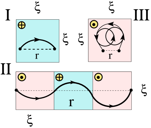
Figure 1: (Color online) Types of semiclassical trajectories between two points separated by a distance, $r$, in a random magnetic field: in the regime I the trajectories are of “arc”-type; in the regime II the trajectories are of “snake”-type; regime III corresponds to a drifting Larmour circle.

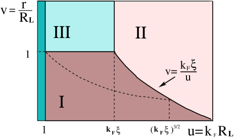
Figure 2: (Color online) Parametric regions for the regimes I, II, and III. Dashed line, $v=u^{-1/3}$, separates slow and fast power-law decays of the averaged Friedel oscillations within the regime I: the oscillations fall off as $1/r^{2}$ to the left from the dashed line, and as $1/r^{7/2}$ to the right from the dashed line.

(i) short-distance regime (regime I in Fig. 1). The trajectory is of the arc-type. For this regime to realize, two conditions must be met. Firstly, the change of magnetic field over the distance, $r$, should be negligible, i.e., $r\ll\xi$. Secondly, the curving of electron trajectory in the locally constant magnetic field must be relative small. The measure of this curving is $r/R_{\text{\tiny{L}}}$, where $R_{\text{\tiny{L}}}=\hbar ck_{\text{\tiny{F}}}/eh_{0}$ is the Larmour radius in the field, $h_{0}$, and $k_{\text{\tiny{F}}}=2\pi/\lambda_{\text{\tiny{F}}}$ is the Fermi momentum. Thus the short-distance regime corresponds to $r\ll\xi,R_{\text{\tiny{L}}}$.

(ii) ”weak-field” long-distance regime (regime II in Fig. 1). The trajectory is of the snake-type. One condition for this regime is that magnetic field changes sign many times within the distance, $r$, i.e., $r\gg\xi$. The other is that within each interval of length $\sim\xi$ the curving of the trajectory is weak, i.e., $\xi\ll R_{\text{\tiny{L}}}$.

(iii) ”strong-field” long-distance regime (regime III in Fig. 1). Electron executes many full Larmour circles before arriving to the point ${\bf r}$. The conditions for this regime are $R_{\text{\tiny{L}}}\ll r$ and $R_{\text{\tiny{L}}}\ll\xi$.

Note, that the last two regimes correspond to the ”semiclassical” and ”strong” random magnetic field regimes in the language of Ref. Mirlin1, . In order to accommodate all three regimes within a single diagram, it is convenient to introduce the dimensionless parameters

$$u=k_{\text{\tiny{F}}}R_{\text{\tiny{L}}}=\left(c\hbar k_{\text{\tiny{F}}}^{2}/eh_{0}\right)={\mathcal{N}}_{h}^{-1},$$

$$v=r/R_{\text{\tiny{L}}}\sim k_{\text{\tiny{F}}}r{\mathcal{N}}_{h},$$ (2)

where ${\mathcal{N}}_{h}<1$ is the flux of the field $h_{0}$ into the area $\lambda_{\text{\tiny{F}}}^{2}$ (in the unites of the flux quantum). Then the regime I is defined by the lines $u=k_{\text{\tiny{F}}}\xi$ and $v=k_{\text{\tiny{F}}}\xi/u$, see Fig. 2. The regime III is separated from the regime I by the line $v=1$, and from the regime II by the line $u=k_{\text{\tiny{F}}}\xi$. Finally, the dashed region $u<1$ in Fig. 2 corresponds to quantizing magnetic field. The diagram Fig. 2 is compiled for $k_{\text{\tiny{F}}}\xi\gg 1$, so it does not reflect white-noise regime, $k_{\text{\tiny{F}}}\xi\ll 1$, of Refs. ioffe, ; meshkov, ; lee, .

III Main results

III.1 Friedel oscillations

The simplest manifestation of the interplay of external field and electron-electron interactions shows up in spatial response of the electron gas to a point-like impurity, or, in other words, in Friedel oscillations. Denote with $U_{imp}({\bf r})$ the short-range potential of the impurity. In the presence of interaction, $V({\bf r}-{\bf r}_{1})$, the effective electrostatic potential in a clean electron gas falls off with $r$ as $V_{\mbox{\tiny H}}(r)\propto\sin(2k_{\mbox{\tiny F}}r)/r^{2}$ in a zero field. In Ref. we1 we had demonstrated that in a constant magnetic field, $h=h_{0}$, this behavior modifies to

$$V_{\mbox{\tiny H}}(r)=-\frac{\nu_{0}gV(2k_{\mbox{\tiny F}})}{2\pi r^{2}}\sin\Biggl{[}2k_{\mbox{\tiny F}}r-\frac{(p_{0}r)^{3}}{12}\Biggr{]},$$ (3)

where the characteristic momentum, $p_{0}$, is defined as

$$p_{0}=\frac{k_{\text{\tiny{F}}}}{(k_{\text{\tiny{F}}}R_{\text{\tiny{L}}})^{2/3}}=\left(\frac{h_{0}}{k_{\mbox{\tiny F}}^{1/2}\Phi_{0}}\right)^{2/3},$$ (4)

where $\Phi_{0}$ is the flux quantum. In Eq. (3) $\nu_{0}=m/\pi\hbar^{2}$ is the free electron density of states, $V(2k_{\mbox{\tiny F}})$ is the Fourier component of $V({\bf r})$, and the parameter $g$ is defined as $g=\int U_{imp}({\bf r})\;d{\bf r}$. Eq. (7) is valid within the domain $k_{\mbox{\tiny F}}^{-1}\lesssim r\lesssim R_{\mbox{\tiny L}}$, so that $(p_{0}r)^{3}/12$ in the argument of sine does not exceed the the main term, $2k_{\mbox{\tiny F}}r$. As follows from Eq. (4), the characteristic length scale,

$$r_{\text{\tiny I}}=\frac{1}{p_{0}}=k_{\mbox{\tiny F}}^{1/3}\left(\frac{\Phi_{0}}{h_{0}}\right)^{2/3},$$ (5)

defied by $p_{0}$, is intermediate between $R_{\mbox{\tiny L}}$ and $\lambda_{\mbox{\tiny F}}$, so that

$$R_{\mbox{\tiny L}}\gg r_{\text{\tiny I}}\gg 1/k_{\mbox{\tiny F}}.$$ (6)

We see from Eq. (3) that only the phase of the Friedel oscillations is affected by the constant field, while the magnitude still falls off as $1/r^{2}$. The randomness of $h(x,y)$ results in randomness of the field-induced phase of the oscillations. This, in turn, translates into a faster decay of disorder-averaged oscillations. To quantify the behavior of the average $\bigl{\langle}V_{\mbox{\tiny H}}(r)\bigr{\rangle}$, we rewrite it the form

$$\bigl{\langle}V_{\mbox{\tiny H}}(r)\bigr{\rangle}=-\frac{\nu_{0}gV(2k_{\mbox{\tiny F}})}{2\pi r^{2}}\;F(r)\sin\Biggl{[}2k_{\mbox{\tiny F}}r+\phi(r)\Biggr{]}\;,$$ (7)

so that $F(r)$ describes the decay of the magnitude of the disorder-averaged oscillations. For a given distance, $r$, the character of the phase randomization is different in the regimes I and II. In regime I, we have $\xi\gg r$, and thus the relevant scale for the decay of $\bigl{\langle}V_{\mbox{\tiny H}}(r)\bigr{\rangle}$ is $r_{\mbox{\tiny I}}$. In Section V we find that in this regime the magnitude, $F_{\text{\tiny I}}$, and the phase, $\phi_{\text{\tiny I}}$, are the following functions of the dimensionless ratio $x=r/r_{\text{\tiny I}}$

$$F_{\text{\tiny I}}(x)=\frac{1}{\left(1+x^{6}\right)^{1/4}},$$ (8)

$$\phi_{\text{\tiny I}}(x)=-\arctan\left[\frac{\sqrt{1+x^{6}}-1}{x^{3}}\right].$$

In regime II, with snake-like trajectories, Fig. 1, the sign of random field changes many, $\sim r/\xi\gg 1$, times within the distance, $r$. As demonstrated in Section V, in this regime we have

$$F_{\text{\tiny II}}(x)=\frac{\sqrt{2}x}{\Bigl{[}1+\frac{4}{9}x^{4}\Bigr{]}^{1/2}\sqrt{\cosh^{2}x-\cos^{2}x}},$$

$$\phi_{\text{\tiny II}}(x)= - \arctan\left[1-\frac{2}{1-\cot x\tanh x}\right]$$ (10)

$$- \arctan\left[\frac{2}{3}x^{2}\right],$$

where $x=r/r_{\text{\tiny II}}$, with $r_{\text{\tiny II}}$ defined as

$$r_{\text{\tiny II}}=\eta~{}\Biggl{(}\frac{k_{\mbox{\tiny F}}}{\xi}\Biggr{)}^{1/2}\frac{\Phi_{0}}{h_{0}}.$$ (11)

In Eq. (11) the numerical factor, $\eta$, depends on the functional form of the correlator Eq. (1) and will be defined in Section V.

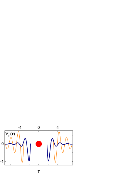
Figure 3: (Color online) Friedel Oscillations of the potential created by an impurity located at the origin. Thick line: averaged Friedel oscillations in regime I is plotted from Eqs. (7), (8). Thin line: oscillations in the absence of the random field [Eq. (3) with $p_{0}=0$].

In conclusion of this subsection we point out that the actual character of the decay of Friedel oscillations with distance is governed by the following dimensionless combination of parameters, $h_{0}$, and, $\xi$, in the correlator Eq. (1) of the random field

$$\varepsilon=\frac{h_{0}^{2}\xi^{3}}{\Phi_{0}^{2}k_{\text{\tiny{F}}}}.$$ (12)

For $\varepsilon\gg 1$, i.e., for strong random field, the averaged oscillations decay with $r$ according to Eq. (8) in the regime I. This is because for $\varepsilon\gg 1$ we have $p_{0}\xi\gg 1$. In the opposite limit of a weak random field, $\varepsilon\ll 1$, we have $p_{0}\xi\ll 1$, so that the scale $p_{0}^{-1}$ is irrelevant, and also no dephasing takes place within the distance, $\xi$. Thus, the characteristic decay length, $r_{\text{\tiny{II}}}\sim\xi/\varepsilon^{1/2}$, is much larger than $\xi$. This automatically guarantees that $k_{\text{\tiny{F}}}r_{\text{\tiny{II}}}\gg 1$.

III.2 Tunnel density of states

Two spatial scales, $r_{\text{\tiny{I}}}$ and $r_{\text{\tiny{II}}}$, define two energy scales,

$$\omega_{0} = \frac{v_{\text{\tiny{F}}}}{r_{\text{\tiny{I}}}}\sim E_{\text{\tiny{F}}}\left(\frac{h_{0}}{\Phi_{0}k_{\text{\tiny{F}}}^{2}}\right)^{2/3}\sim E_{\text{\tiny{F}}}{\mathcal{N}}_{h}^{2/3},$$ (13)

$$\omega_{1} = \frac{v_{\text{\tiny{F}}}}{r_{\text{\tiny{II}}}}\sim E_{\text{\tiny{F}}}\left(\frac{\xi^{1/2}h_{0}}{k_{F}^{2/3}\Phi_{0}}\right)\sim E_{\text{\tiny{F}}}\left(k_{\text{\tiny{F}}}\xi\right)^{1/2}{\mathcal{N}}_{h}.$$

As shown below, these scales manifest themselves in the anomalous behavior of the density of states in the third order in the electron-electron interaction parameter, $\nu_{0}V$. More specifically, in the regime I, the bare density of states, $\nu_{0}$, acquires a correction $\delta\nu_{\text{\tiny{I}}}(\omega)\sim\nu_{0}(\nu_{0}V)^{3}\left(\omega_{0}/E_{\text{\tiny{F}}}\right)^{3/2}{\mathcal{I}}\left(\omega/\omega_{0}\right)$, where $E_{\text{\tiny{F}}}$ is the Fermi energy. In the regime II the correction has a similar form $\delta\nu_{\text{\tiny{II}}}(\omega)\sim\nu_{0}(\nu_{0}V)^{3}\left(\omega_{1}/E_{\text{\tiny{F}}}\right)^{3/2}{\mathcal{J}}\left(\omega/\omega_{1}\right)$. Both functions, ${\mathcal{I}}(z)$ and ${\mathcal{J}}(z)$, have characteristic magnitude and scale $\sim 1$. Moreover, they exhibit quite a ”lively” behavior. In particular, a zero-bias anomaly, $\delta\nu_{\text{\tiny{I}}}(\omega)$, falls off at $\omega\gg\omega_{0}$ with aperiodic oscillations, i.e., ${\mathcal{I}}(z)$ has a contribution $\propto{\sin\left(2^{8/3}\sqrt{3}z\right)}z^{-3/4}\exp\left\{-2^{8/3}z\right\}$ for $z\gg 1$. The origin of the oscillations is the power-law decay of $F_{\text{\tiny{I}}}(x)$, given by Eq. (8), and the brunch-point, $x=e^{i\pi/6}$.

The contribution, $\delta\nu_{\text{\tiny{II}}}(\omega)$, also has a non-monotonic behavior, despite the fact that $F_{\text{\tiny{II}}}(x)$ falls off exponentially, as $\exp(-r/r{\text{\tiny{II}}})$ [see Eq. (III.1)].

It is instructive to trace the evolution of the zero-bias anomaly upon increasing the magnitude of the random field, $h_{0}$. This evolution is governed by parameter, $\varepsilon$, Eq. (12). While $\varepsilon$ remains smaller than one, where the regime II applies, the anomaly is described by the function ${\mathcal{J}}(\omega/\omega_{1})$ and broadens with $h_{0}$ as $v_{\text{\tiny{F}}}/r_{\text{\tiny{II}}}(h_{0})\propto h_{0}$. Upon further increasing $h_{0}$, when $\varepsilon$ exceeds one, the crossover to the regime I takes place. Zero-bias anomaly is then described by ${\mathcal{I}}(\omega/\omega_{0})$; it broadens with $h_{0}$ as $v_{\text{\tiny{F}}}/r_{\text{\tiny{I}}}(h_{0})\propto h_{0}^{2/3}$, and develops oscillations. The fact that oscillations in $\delta\nu(\omega)$ emerge upon strengthening disorder might seem counterintuitive. This issue will be discussed in details in Section VII.

In a zero magnetic field, an intimate relation between impurity-induced Friedel oscillations and the zero-bias anomaly was first established in Ref. rudin97, . Namely, it was demonstrated that for short-range interaction $\delta\nu(\omega)/\nu_{0}\sim(\nu_{0}V/E_{\text{\tiny{F}}}\tau)\ln\omega$, where $1/\tau=\nu_{0}\pi g^{2}n_{\text{imp}}$ is the electron scattering rate by the impurities, and $n_{\text{imp}}$ is the impurity concentration. This anomaly is of the first order in $V$. A non-trivial question is whether or not the modification, Eq. (3), in a constant magnetic field results in field dependence of the density of states in this order. In other words, whether or not a weak magnetic field introduces a cutoff of $\ln\omega$ at small $\omega$. The answer to this question is negative. In Ref. we1, it was demonstrated that sensitivity of $\delta\nu(\omega)$ to a weak magnetic field indeed emerges, but in the second order in $\nu_{0}V$ (however, still in the first order in $1/\tau$). The field-dependent correction, $\left[\delta\nu(\omega,h)-\delta\nu(\omega,0)\right]/\nu_{0}$, has a characteristic frequency scale, $\omega=\omega_{0}$. It is interesting to note that, at $\omega\gg\omega_{0}$, this impurity-induced correction has an oscillating character

$$\frac{\delta\nu(\omega,h)-\delta\nu(\omega,0)}{\nu_{0}}=\frac{(\nu_{0}V)^{2}}{E_{\text{\tiny{F}}}\tau}\left(\frac{\omega_{0}}{E_{\text{\tiny{F}}}}\right)^{1/2}{\text{\Large P}}\left(\frac{\omega}{\omega_{0}}\right).$$

The dimensionless function, P, has the following large-$x$ asymptote

$${\text{\Large P}}(x)\propto\frac{1}{x^{3/4}}\cos\left[\frac{8}{3\sqrt{3}}x^{3/2}-\frac{\pi}{4}\right].\;\;\;$$ (15)

In Fig. 4 we show the oscillating correction to the density of states; the form of the function ${\text{\large P}}\left(\omega/\omega_{0}\right)$ is addressed in Section VII. Technically, the derivation of Eqs.  (III.2), (15) is quite analogous to the derivation of the oscillatory $\delta\nu$ in the random field in the regime I. For this reason we will outline this derivation in Section VII.

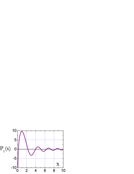
Figure 4: (Color online) Magnetic-field-induced contribution Eq. (93) to the ballistic zero-bias anomaly Eq. (III.2). Field-dependent correction, $\left[\delta\nu(\omega,h)-\delta\nu(\omega,0)\right]/\nu_{0}$, in the units $(\nu_{0}V)^{2}(\omega_{0}/E_{\text{\tiny{F}}})^{1/2}(E_{\text{\tiny{F}}}\tau)^{-1}$ is plotted versus dimensionless energy $2^{2/3}(\omega/\omega_{0})$, where $\omega_{0}=(2E_{\text{\tiny{F}}})^{1/3}\omega_{c}^{2/3}\gg\omega_{c}$, and $\omega_{c}$ is the cyclotron frequency.

IV Polarization operator in a random magnetic field

Friedel oscillations, $V_{\mbox{\tiny H}}(r)$, created by a point-like impurity, and the ballistic zero-bias anomaly originating from these oscillationsrudin97 are intimately related to the Kohn anomaly in the polarization operator, $\Pi(q)$, of a clean electron gas near $q=2k_{\text{\tiny{F}}}$. In two dimensions, this anomaly behaves as Stern67 $(q-2k_{\text{\tiny{F}}})^{1/2}$, which translates into $1/r^{2}$ decay of the Friedel oscillations and $\propto\ln\omega$ correction to the density of states. Suppression of the Friedel oscillations, $V_{\mbox{\tiny H}}(r)$, in a random field is a result of smearing of the Kohn anomaly in the momentum space. However, since the momentum is not a good quantum number in the presence of the random field, it is much more convenient to study the field-induced suppression of $V_{\mbox{\tiny H}}(r)$ directly in the coordinate space.

IV.1 Evaluation in the coordinate space

Polarization operator, $\Pi_{\Omega}({\bf r},{\bf r}^{\prime})$, is defined in a standard way as

$$\Pi({\bf r},{\bf r}^{\prime},\Omega)=-i\int\frac{d\Omega^{\prime}}{2\pi}G_{\Omega^{\prime}}({\bf r},{\bf r}^{\prime})G_{\Omega-\Omega^{\prime}}({\bf r}^{\prime},{\bf r}).$$ (16)

Here $G_{\Omega}({\bf r},{\bf r}^{\prime})$ denotes causal Green function, which coincides with the retarded, $G_{\Omega}^{R}({\bf r},{\bf r}^{\prime})$, or advanced $G_{\Omega}^{A}({\bf r},{\bf r}^{\prime})$ Green functions for $\Omega>0$ and $\Omega<0$, respectively. At distances $|{\bf r}-{\bf r}^{\prime}|\gg k_{\text{\tiny{F}}}^{-1}$ the polarization operator in coordinate space represents the sum $\Pi_{0}(r,\omega)$ and $\Pi_{2k_{\text{\tiny{F}}}}(r,\omega)$ of slow and rapidly oscillating parts

$$\Pi_{0}(r,\omega)=-\frac{i\pi\nu_{0}^{2}\hbar^{4}}{2k_{\mbox{\tiny F}}r}|\omega|\exp\left\{\frac{i|\omega|r}{v_{\mbox{\tiny F}}}\right\},$$ (17)

$$\Pi_{2k_{\text{\tiny{F}}}}(r,\omega)=-\frac{\nu_{0}\hbar^{3}}{2r^{2}}\sin\bigl{(}2k_{\text{\tiny{F}}}r\bigr{)}A\Biggl{(}\frac{2\pi rT}{v_{\mbox{\tiny F}}}\Biggr{)}$$

$$\times\exp\left\{\frac{i|\omega|r}{v_{\mbox{\tiny F}}}\right\}.$$ (18)

Subindices $0$ and $2k_{\text{\tiny{F}}}$ emphasize that these parts come from small momenta and momenta close to $2k_{\text{\tiny{F}}}$ in $\Pi(q)$, respectively. Eq. (17) emerges if one of the Green functions in Eq. (16) is retarded and the other is advanced. Eq. (IV.1) corresponds to the case when the Green functions in Eq. (16) are both advanced or both retarded Chubukov1 ; Chubukov2 . Derivation of Eqs. (17), (IV.1) is presented in Appendix A. In Eq. (IV.1) the function,

$$A(x)=\frac{x}{\sinh x},$$ (19)

in $\Pi_{2k_{\text{\tiny{F}}}}$ describes the temperature damping.

IV.2 Qualitative derivation for the constant field

For a constant magnetic field, $h(x,y)\equiv h_{0}$, the phase, $\phi(r)$, in the argument of Eq. (7) can be inferred from the following simple qualitative consideration.

Classical trajectory of an electron in a weak magnetic field is curved due to the Larmour motion even at the spatial scales much smaller than $R_{\mbox{\tiny L}}$. As a result of this curving, the electron propagator, $G({\bf r}_{1},{\bf r}_{2})$, between the points ${\bf r}_{1}$ and ${\bf r}_{2}$ contains, in the semiclassical limit, a phase, $k_{\mbox{\tiny F}}{\cal L}$, where ${\cal L}$ is the length of the arc of a circle with the radius $R_{\mbox{\tiny L}}$, that connects the points ${\bf r}_{1}$ and ${\bf r}_{2}$, see Fig. 5a. Since the Friedel oscillations are related to the propagation from ${\bf r}_{1}$ to ${\bf r}_{2}$ and back, it is important that two arcs, corresponding to the opposite directions of propagation, define a finite area, $\cal A$, so that the product $G({\bf r}_{1},{\bf r}_{2})G({\bf r}_{2},{\bf r}_{1})$ should be multiplied by the Aharonov-Bohm phase factor, $\exp\left[ih_{0}{\cal A}/\Phi_{0}\right]$. Then the phase, of this product is equal to

$$2k_{\text{\tiny{F}}}r+\phi(r)=2k_{\mbox{\tiny F}}{\cal L}-\frac{h_{0}{\cal A}({\bf r}_{1},{\bf r}_{2})}{\Phi_{0}}.$$ (20)

Simple geometrical relations, see Fig. 5a, yield

$$r=|{\bf r}_{1}-{\bf r}_{2}|=2R_{\mbox{\tiny L}}\sin(\delta/2),$$

$${\cal L}=R_{\mbox{\tiny L}}\delta,\;\;\;\;{\cal A}=2R_{\mbox{\tiny L}}^{2}(\delta-\sin\delta).$$ (21)

Using this relation and assuming $r\ll R_{\mbox{\tiny L}}$, we find

$$\phi(r)=-\frac{h_{0}^{2}r^{3}}{12k_{\text{\tiny{F}}}\Phi_{0}^{2}}=-\frac{(p_{0}r)^{3}}{12}.$$ (22)

At this point, we would like to note, that the conventional way gorkov59 of incorporating magnetic field into the semiclassical zero-field Green’s function amounts to multiplying it by $\exp\left[(1/\Phi_{0})\int{\bf a}\cdot d{\bf l}\right]$, where the phase factor is the integral of the vector potential, ${\bf a}$, along the straight line, connecting the points ${\bf r}_{1}$ and ${\bf r}_{2}$. Such an incorporation neglects the field-induced curvature of the electron trajectories, and thus does not capture the modification Eq. (7) of the Friedel oscillations in magnetic field. Indeed, the magnetic phase factors, introduced following Ref. gorkov59, cancel out in the polarization operator.

With phase, $\phi(r)$, given by Eq. (22), Friedel oscillations in a constant magnetic field acquire the formwe1 Eq. (3). To see this, we notice that, with accuracy of a factor, $g/2\pi$, the potential, $V_{\text{\tiny{H}}}(r)$ coincides with $\Pi_{2k_{\text{\tiny{F}}}}(r,0)$. Then the additional phase Eq. (22) transforms $\sin(2k_{\text{\tiny{F}}}r)$ into $\sin\left[2k_{\text{\tiny{F}}}r-(p_{0}r)^{3}/12\right]$, as in Eq. (3).

In Appendix B we present a rigorous derivation of Eq. (3) starting from exact electronic states in a constant magnetic field, as in Ref. aleiner95, .

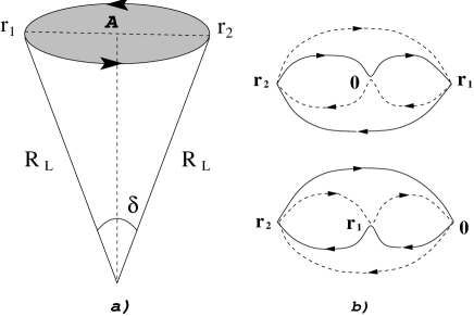
Figure 5: (a) Origin of the net “magnetic” phase Eq. (22): two arcs, corresponding to the opposite directions of propagation, define a finite area, ${\cal A}$. Aharonov-Bohm flux through this area makes the net phase negative; (b) Schematic illustration of the scattering processes giving rise to the additional phases Eqs. (74), (75) in the product Eq. (VII.2).

IV.3 Field-induced phase of the Green function: Analytical derivation in a spatially-inhomogeneous field

Additional semiclassical phase, $\delta\varphi_{0\rightarrow{\bf r}}$, of the Green function due to the random magnetic field, $h(x,y)$, is given by the following generalization of Eq. (22)

$$\delta\varphi_{0\rightarrow{\bf r}}=\frac{k_{\text{\tiny{F}}}}{2}\int_{0}^{r}dx\Biggl{(}\frac{dy}{dx}\Biggr{)}^{2}-\frac{1}{\Phi_{0}}\int_{0}^{r}\!dx\;y(x)\;h(x,0),$$ (23)

where the first term comes from the elongation of the trajectory in magnetic field. The second term describes the Aharonov-Bohm flux into the area restricted by the curve $y(x)$ and the $x$-axis. In Eq. (23) we assumed that the field does not change along the $y$-axis. This is the case when the maximal $y$ is smaller than the correlation radius, $\xi$, of the random field. The condition $y<\xi$ is met in the regime of the ”arcs” and the regime of the ”snakes”, see Figs. 1, 2.

In Eq. (23) we have also assumed that the magnitude of the de Broglie wavelength of the electron does not change along the trajectory. This can be justified from the equations of motion

$$m\frac{d^{2}y}{dt^{2}}\!\! = \!\!\frac{e}{c}\;h(x,0)\frac{dx}{dt}$$

$$m\frac{d^{2}x}{dt^{2}}\!\! = \!\!-\frac{e}{c}\;h(x,0)\frac{dy}{dt}.$$ (24)

It follows from Eq. (IV.3) that the energy of electron $\frac{m}{2}[(dx/dt)^{2}+(dy/dt)^{2}]$ is conserved even if magnetic field changes with coordinates.

The most important step that allows to find $\delta\varphi_{0\rightarrow{\bf r}}$ analytically, is that in the regimes I and II in Fig. 1 we can replace $dx/dt$ by $v_{\text{\tiny{F}}}$ and set $t=x/v_{\text{\tiny{F}}}$ in the rhs of Eq. (IV.3). This allows to replace $d^{2}y/dt^{2}$ by $v_{\text{\tiny{F}}}^{2}d^{2}y/dx^{2}$. Then the first of the equations yields

$$mv_{\text{\tiny{F}}}^{2}\frac{d^{2}y}{dx^{2}}=\frac{ev_{\text{\tiny{F}}}}{c}h(x,0).$$ (25)

Integrating this equation, we obtain

$$\frac{dy}{dx}=\frac{e}{mcv_{\text{\tiny{F}}}}\int_{0}^{x}\!dx^{\prime}h(x^{\prime},0)+C.$$ (26)

The constant, $C$, should be found from the conditions: $y(0)=0$, and $y(r)=0$, leading to

$$C=-\frac{e}{mcv_{\text{\tiny{F}}}r}\int_{0}^{r}dx^{\prime}\int_{0}^{x^{\prime}}dx^{\prime\prime}h(x^{\prime\prime},0)$$

$$=-\frac{e}{mcv_{\text{\tiny{F}}}r}\int_{0}^{r}dx^{\prime}\Lambda(x^{\prime}),$$ (27)

where we have introduced an auxiliary function

$$\Lambda(x)=\int_{0}^{x}\!dx^{\prime}h(x^{\prime},0).$$ (28)

The meaning of $\Lambda(x)$ is the $y$-projection of the vector potential. Substituting Eq. (IV.3) back into Eq. (26), we find

$$\frac{dy}{dx}=\frac{e}{mcv_{\text{\tiny{F}}}}\Biggl{[}\int_{0}^{x}\!dx^{\prime}h(x^{\prime},0)\qquad\qquad\qquad\qquad\qquad$$

$$\qquad\qquad\qquad\qquad\qquad-\frac{1}{r}\int_{0}^{r}\!dx^{\prime}\int_{0}^{x^{\prime}}dx^{\prime\prime}h(x^{\prime\prime},0)\Biggr{]}$$

$$=\frac{e}{mcv_{\text{\tiny{F}}}}\Biggl{[}\Lambda(x)-\frac{1}{r}\int_{0}^{r}\!dx\Lambda(x)\Biggr{]}.\qquad\qquad\qquad$$ (29)

With the help of Eq. (IV.3) one can express the first term in additional phase Eq. (23) in terms of $\Lambda(x)$. It turns out that the second term in Eq. (23) exceeds twice the first term. To see this, one should multiply the first of equations Eq.  (IV.3) by $y(x)$ and integrate over $x$

$$\int_{0}^{r}dx\;y(x)\;\frac{d^{2}y}{dx^{2}}=\frac{1}{\Phi_{0}k_{\text{\tiny{F}}}}\int_{0}^{r}dx\;h(x,0)\;y(x).$$ (30)

The rhs of Eq. (30) is the second term in Eq. (23). The lhs of Eq. (30) can be related to the first term in Eq. (23) upon integration by parts

$$\int_{0}^{r}\!dx\;y(x)\frac{d^{2}y}{dx^{2}}=-\int_{0}^{r}dx\left(\frac{dy}{dx}\right)^{2}.$$ (31)

Finally, we get

$$\delta\varphi_{0\rightarrow{\bf r}}=-\frac{k_{\text{\tiny{F}}}}{2}\int_{0}^{r}dx\left(\frac{dy}{dx}\right)^{2}\qquad\qquad\qquad\qquad\qquad$$ (32)

$$=-\frac{1}{\Phi_{0}^{2}k_{\text{\tiny{F}}}}\Biggl{(}\int_{0}^{r}dx\;\Lambda^{2}(x)-\frac{1}{r}\left[\int_{0}^{r}dx\;\Lambda(x)\right]^{2}\Biggr{)}.$$

It is convenient to rewrite the final result Eq. (32) directly in terms of the random field, $h({\bf r})$. Substituting Eq. (28) into Eq. (32), we obtain

$$\delta\varphi_{0\rightarrow{\bf r}}=\frac{1}{\Phi_{0}^{2}k_{\text{\tiny{F}}}\xi}\int d{\bf r_{1}}\int d{\bf r_{2}}h({\bf r_{1}}){\cal R}({\bf r_{1}},{\bf r_{2}})h({\bf r_{2}}),\;\;\;\;\;$$ (33)

where the dimensionless kernel ${\cal R}({\bf r}_{1},{\bf r}_{2})$ is defined as

$${\cal R}({\bf r_{1}},{\bf r_{2}})=\xi\;\delta(y_{1})\;\delta(y_{2})\qquad\qquad\qquad\qquad$$ (34)

$$\times\left[r-\frac{x_{1}x_{2}}{r}-x_{2}\;\theta(x_{2}-x_{1})-x_{1}\;\theta(x_{1}-x_{2})\right].$$

Note, that for the constant field $h(x,y)=h_{0}$, evaluation of Eq. (33) using the kernel Eq. (34) reproduces the result Eq. (22), as expected.

V Disorder-smeared Friedel oscillations in different regimes

Smearing of the Friedel oscillations in the random field, $h({\bf r})$, originates from the randomness of the phase, $\varphi_{0\rightarrow{\bf r}}$, which is related to $h({\bf r})$ via Eqs. (33), (34). Quantitatively, the magnitude, $F(r)$, and the phase, $\phi(r)$, of smeared Friedel oscillations Eq. (7) are determined by the following averages

$$\Upsilon_{1}(r)=\text{Im}\bigl{\langle}e^{2i\delta\varphi_{0\rightarrow{\bf r}}}\bigr{\rangle}_{h({\bf r})},~{}\Upsilon_{2}(r)=\text{Re}\bigl{\langle}e^{2i\delta\varphi_{0\rightarrow{\bf r}}}\bigr{\rangle}_{h({\bf r})}.$$

Then $F(r)$ and $\phi(r)$ are related to the functions $\Upsilon_{1}(r)$ and $\Upsilon_{2}(r)$ as

$$F(r)=\sqrt{\bigl{[}\Upsilon_{1}(r)\bigr{]}^{2}+\bigl{[}\Upsilon_{2}(r)\bigr{]}^{2}},$$

$$\phi(r)=\arctan\left[\frac{\Upsilon_{1}(r)}{\Upsilon_{2}(r)}\right].$$ (36)

In this Section the averages Eq. (V) will be calculated separately for the regime of ”arcs” and the regime of ”snakes”.

V.1 Regime I

In the regime of “arcs” we have $r\ll\xi$, so that the field is almost constant within the interval $(0,r)$ and is equal to its “local” value. For this reason, we can perform the averaging of $\exp\left[2i\varphi_{0\rightarrow{\bf r}}\right]$ over realizations of the random field, $h(x,y)$, explicitly, without specifying the form of the correlator, $\text{\large K}(r/\xi)$. This is because we can first set $h(x,y)\equiv const$ in $\exp\left[2i\varphi_{0\rightarrow{\bf r}}\right]$, and then make use of the fact that the distribution function of the local field is Gaussianwe2 . Characteristic spatial scale, $r_{\text{\tiny{I}}}$, for $F(r)$ and $\phi(r)$ immediately follows from Eq. (33) upon setting $h(0,r)=h_{0}$, and requiring $2\delta\varphi_{0\rightarrow{\bf r}}=1$. This yields $r_{\text{\tiny{I}}}=2^{2/3}3^{1/3}/p_{0}$, where $p_{0}$ is given by Eq. (4).

V.1.1 Random magnetic field

As discussed above, we start with Friedel oscillations in a constant local magnetic field, $h$, for which we know that

$$F_{\text{\tiny{I}}}(r,h)=1,~{}~{}~{}~{}~{}\phi_{\text{\tiny{I}}}(r,h)=-\epsilon_{r}\left(\frac{h}{h_{0}}\right)^{2},$$ (37)

where $p_{0}=k_{\text{\tiny{F}}}(\omega_{c}/E_{\text{\tiny{F}}})^{2/3}$, and $\omega_{c}=eh_{0}/mc$ is the cyclotron frequency in the field, $h_{0}$. In Eq. (37) the parameter, $\epsilon_{r}$, is defined as

$$\epsilon_{r}=\frac{h_{0}^{2}r^{3}}{12\Phi_{0}^{2}k_{\text{\tiny{F}}}}=\frac{(p_{0}r)^{3}}{12}.$$ (38)

To find the form of the averaged Friedel oscillation in the regime I, in which $p_{0}\xi\ll 1$, we have to simply substitute the “local” value, $h$, of magnetic field into Eq. (3), i.e., replace $p_{0}^{3}$ by $p_{0}^{3}h^{2}/h_{0}^{2}$, and perform the gaussian averaging over the distribution of the local field. This averaging can be carried out analytically with the use of identity

$$\int\limits_{-\infty}^{\infty}\!\!\!\frac{dx}{\sqrt{\pi}}~{}e^{-x^{2}}\!\!\cos(\epsilon_{r}x^{2}+\beta)\!=\!\Upsilon_{1}(\epsilon_{r})\cos\beta-\Upsilon_{2}(\epsilon_{r})\sin\beta,$$

where the functions $\Upsilon_{1}$ and $\Upsilon_{2}$ for this case assume the following forms

$$\Upsilon_{1}\rightarrow\Biggl{(}\frac{\pi}{2}\Biggr{)}^{1/2}\sqrt{\frac{(1+\epsilon_{r}^{2})^{1/2}+1}{1+\epsilon_{r}^{2}}},$$ (40)

$$\Upsilon_{2}\rightarrow\Biggl{(}\frac{\pi}{2}\Biggr{)}^{1/2}\sqrt{\frac{(1+\epsilon_{r}^{2})^{1/2}-1}{1+\epsilon_{r}^{2}}}.$$ (41)

Using Eq. (V), we recover from Eqs. (40), (41) the final result Eq. (8) for the magnitude $F_{\text{\tiny{I}}}(r/r_{\text{\tiny{I}}})$ and the phase $\phi_{\text{\tiny{I}}}(r/r_{\text{\tiny{I}}})$ of the Friedel oscillations in the regime I.

In terms of variables $u$ and $v$ in the parametric space Fig. 2, the condition $\epsilon_{r}=1$ can be presented as

$$v=\frac{1}{u^{1/3}},\;\;\text{where}\;\;\;u=k_{\text{\tiny{F}}}R_{\text{\tiny{L}}},\;\;v=\frac{r}{R_{\text{\tiny{L}}}}.$$ (42)

The dependence Eq. (42) is shown in Fig. 2 with a dashed line within the regime I. To the left of this line, we have $\epsilon_{r}<1$, so that $1/r^{2}$ decay of the Friedel oscillations is unchanged in the random field. To the right of the dashed line, $\epsilon_{r}$ is bigger than $1$. Then, the dependence $F(r)\propto\epsilon_{r}^{-1/2}$, which follows from Eq. (8), translates into faster, but still power-law decay, $\propto 1/r^{7/2}$, of the Friedel oscillations. Note also, that the phase of the oscillations also changes as $\epsilon_{r}$ crosses over from small to large values. Indeed, as follows from Eq. (8), we have $\phi(r)\rightarrow-\pi/4+1/(2r^{3})$ in the limit $\epsilon_{r}\gg 1$.

V.1.2 Periodic Magnetic Field

Consider a particular case of a spatially-periodic magnetic field $h(x,y)={\tilde{h}}_{0}\cos(qx)$. For small enough $q$ the “local” description applies. The corresponding condition reads

$$q\ll{\tilde{p}}_{0}=k_{\text{\tiny{F}}}\Bigl{(}\frac{{\tilde{h}}_{0}}{k_{\text{\tiny{F}}}^{2}\Phi_{0}}\Bigr{)}^{2/3}.$$ (43)

Under this condition, the averaged Friedel oscillation can be found by averaging

Eq. (3), in which $p_{0}$ is replaced by $\tilde{p}_{0}\left(h/\tilde{h}_{0}\right)^{2/3}$, over the distribution, $P(h)$, of the local values of magnetic field rather than over the gaussian distribution Eq. (V.1.1). This distribution has the form

$$P(h)=\frac{1}{\pi\sqrt{{\tilde{h}}_{0}^{2}-h^{2}}},$$ (44)

so that instead of Eq. (V.1.1) we have

$$\frac{1}{\pi}\int\limits_{-1}^{1}dx\frac{\cos({\tilde{\epsilon}}_{r}x^{2}+\beta)}{\sqrt{1-x^{2}}}=J_{0}\left({\tilde{\epsilon}}_{r}/2\right)\cos\left(\frac{{\tilde{\epsilon}}_{r}}{2}+\beta\right)\;\;\;$$

$$={\tilde{\Upsilon}}_{1}({\tilde{\epsilon}}_{r})\cos\beta-{\tilde{\Upsilon}}_{2}({\tilde{\epsilon}}_{r})\sin\beta,\;\;\;\;$$ (45)

where $J_{0}$ is the Bessel function, $\tilde{\varepsilon}_{r}=\left(\tilde{p}_{0}r\right)^{3}/12$, and

$${\tilde{\Upsilon}}_{1}({\tilde{\epsilon}}_{r})=J_{0}\left(\frac{{\tilde{\epsilon}}_{r}}{2}\right)\cos\left(\frac{{\tilde{\epsilon}}_{r}}{2}\right),$$ (46)

$${\tilde{\Upsilon}}_{2}({\tilde{\epsilon}}_{r})=J_{0}\left(\frac{{\tilde{\epsilon}}_{r}}{2}\right)\sin\left(\frac{{\tilde{\epsilon}}_{r}}{2}\right),$$

so that in a periodic field, instead of Eq. (8), we have

$${\tilde{F}}(r)=\Bigl{[}{\tilde{\Upsilon}}_{1}^{2}({\tilde{\epsilon}}_{r})+{\tilde{\Upsilon}}_{2}^{2}({\tilde{\epsilon}}_{r})\Bigr{]}^{1/2}=\left|J_{0}\left(\frac{{\tilde{\epsilon}}_{r}}{2}\right)\right|,$$ (47)

$$\tilde{\phi}(r)=-\arctan\left[\frac{{\tilde{\Upsilon}}_{2}({\tilde{\epsilon}}_{r})}{{\tilde{\Upsilon}}_{1}({\tilde{\epsilon}}_{r})}\right]=-\frac{{\tilde{\epsilon}}_{r}}{2}.$$

It is instructive to present the results Eq. (47) in a different form, by simply showing how the Friedel oscillation Eq. (3) gets modified on average in the presence of a periodic magnetic field. Substituting Eq. (47) into Eq. (7) we get

$$\Bigl{\langle}V_{\mbox{\tiny H}}(r)\Bigr{\rangle} = -\frac{\nu_{0}gV(2k_{\mbox{\tiny F}})}{2\pi r^{2}}\;J_{0}\left(\frac{{\tilde{p}}_{0}^{3}r^{3}}{24}\right)\qquad\qquad$$ (48)

$$\times \sin\Biggl{[}2k_{\mbox{\tiny F}}r-\frac{({\tilde{p}}_{0}r)^{3}}{24}\Biggr{]}.$$

Eq. (48) is a quite remarkable result. It suggests that, due to the periodic smooth magnetic field, the averaged Friedel oscillations do not get smeared. Rather they acquire an oscillatory envelope, $J_{0}\left(\frac{{\tilde{p}}_{0}^{3}r^{3}}{24}\right)$. This envelope oscillates with “period”much larger than the de Broglie wave length, but much smaller than the period, $1/q$, of change of the magnetic field.

Note that this effect provides a unique possibility to measure experimentally the amplitude of a periodic modulation. The reason is the following. The envelop Eq. (48) due to periodic magnetic field (or electric field, i.e., due to the lateral superlattice) translates into a distinct low-frequency behavior of the tunnel density of states. Namely, the tunnel density of states would exhibit an “oscillatory”behavior with a “period” $\omega\sim{\tilde{p}}_{0}v_{\text{\tiny{F}}}$. This period in $\omega$ depends only on the magnitude of the modulation, ${\tilde{h}}_{0}$, but not on the spatial period of modulation, $2\pi/q$. Therefore, the magnitude of modulation, which, unlike the period, is hard to measure otherwise, can be inferred from the bias dependence of the tunneling conductance.

V.2 Friedel oscillations in a random magnetic field: Regime II

As the magnitude, $h_{0}$, of the random field decreases, the character of semiclassical motion changes from arc-like (regime I in Fig. 1) to the snake-like (regime II in Fig. 1). To estimate for the ”widths”, $\delta y$, of the snake-like trajectories, we use Eq. (IV.3) and set $x\sim\xi$. This yields

$$\frac{\delta y}{\xi}\sim\frac{eh_{0}\xi}{mcv_{\text{\tiny{F}}}}\sim\left(\frac{\epsilon}{k_{\text{\tiny{F}}}\xi}\right)^{1/2}.$$ (49)

Since $k_{\text{\tiny{F}}}\xi\gg 1$ and $\epsilon\ll 1$ in regime II, we confirm that $\delta y\ll\xi$, i.e., that the snake is ”narrow”.

It is clear that at large enough distances, $r$, the magnitude, $F(r)$, of the averaged Friedel oscillations falls off exponentially with $r$. The prime question is what is the characteristic decay length. As stated in Section III this length, $r_{\text{\tiny{II}}}$, is given by Eq. (11). Below we derive this length qualitatively, and then establish the form of the magnitude, $F_{\text{\tiny{II}}}(r)$, as well as the phase, $\phi_{\text{\tiny{II}}}(r)$, for the average Friedel oscillations within the entire domain of $r$ by performing the functional averaging of $\exp(2i\delta\varphi_{0\rightarrow{\bf r}}).$

V.2.1 Qualitative consideration

To recover qualitatively the scale $r_{\text{\tiny{II}}}$ from Eq. (33) we consider the following toy model. Let us divide the interval $(0,r)$ into small intervals of a fixed length, $\xi$ (overall, $r/\xi$ intervals). Assume now that the random field takes only two values, $h_{0}$ and $-h_{0}$, each with probability, $1/2$, within a given interval, $\xi$. Under this assumption, we find from Eq. (28) $\Lambda(r)=h_{0}\left[m(r)-n(r)\right]\xi$, where $m(r)$ and $n(r)$ are the numbers of small intervals within the length, $r$, with $h=h_{0}$ and $h=-h_{0}$, respectively (obviously, $m+n=r/\xi$). From Eq. (32) we get for $\delta\varphi_{0\rightarrow{\bf r}}$

$$\delta\varphi_{0\rightarrow{\bf r}} = \frac{h_{0}^{2}\xi^{2}}{\Phi_{0}^{2}k_{\text{\tiny{F}}}}\Biggl{\{}\int_{0}^{r}dx\bigl{[}m(x)-n(x)\bigr{]}^{2}$$ (50)

$$- \frac{1}{r}\left(\int_{0}^{r}dx\bigl{[}m(x)-n(x)\bigr{]}\right)^{2}\Biggr{\}}.$$

Second term in Eq. (50) is square of the difference $\langle m\rangle-\langle n\rangle$ of coordinate (not statistical) average values of $m(x)$ and $n(x)$. Rewriting $m(x)$ as $\langle m\rangle+\delta m(x)$ and $n(x)$ as $\langle n\rangle+\delta n(x)$, and taking into account that $\delta m(x)+\delta n(x)=0$, one can cast Eq. (50) into the form

$$\delta\varphi_{0\rightarrow{\bf r}}=\frac{4h_{0}^{2}\xi^{2}}{\Phi_{0}^{2}k_{\text{\tiny{F}}}}\int_{0}^{r}dx\left[\delta m(x)\right]^{2}.$$ (51)

Since the typical value of $\left[\delta m(x)\right]^{2}$ is $\langle m(x)\rangle=x/2\xi$, we arrive at the following estimate $\delta\varphi_{0\rightarrow{\bf r}}\sim h_{0}^{2}\xi r^{2}/\Phi_{0}^{2}k_{\text{\tiny{F}}}$. Equating this additional phase to unity yields $r=\Phi_{0}k_{\text{\tiny{F}}}^{1/2}/h_{0}\xi^{1/2}$, which coincides with $r_{\text{\tiny{II}}}$ defined by Eq. (11) within a numerical factor.

V.2.2 Evaluation of the functional integral

Below we present the analytical derivation of Eqs. (III.1), (10). The averaging of $\exp\left(2i\delta\varphi_{0\rightarrow{\bf r}}\right)$ required to calculate $F_{\text{\tiny{II}}}(r)$, and $\phi_{\text{\tiny{II}}}(r)$ from Eqs. (V), (V) reduces to the functional integral

$$\bigl{\langle}e^{2i\delta\varphi_{0\rightarrow{\bf r}}}\bigr{\rangle}=\frac{\int D\left\{h({\bf r})\right\}\exp\Bigl{[}2i\delta\varphi({\bf r})-W\left\{h({\bf r})\right\}\Bigr{]}}{\int D\left\{h({\bf r})\right\}\exp\Bigl{[}-W\left\{h({\bf r})\right\}\Bigr{]}},$$

where $\delta\varphi(r)=\delta\varphi_{0\rightarrow{\bf r}}$ is given by Eq. (32), and $\exp\left(-W\{h\}\right)$ with $W\left\{h({\bf r})\right\}$ given by

$$W\{h\}=\frac{1}{\xi^{4}h_{0}^{2}}\int_{0}^{r_{2}}\int_{-\infty}^{\infty}dx_{1}\;dy_{1}\int_{0}^{r_{2}}\int_{-\infty}^{\infty}dx_{2}\;dy_{2}\;\qquad$$

$$\times\;h(x_{1},y_{1})h(x_{2},y_{2})\;\kappa(x_{1}-x_{2},y_{1}-y_{2}),\quad\qquad$$ (53)

is the statistical weight of the realization, $h(x,y)$. The dimensionless function $\kappa({\bf r},{\bf r}^{\prime})$ is related to the correlator Eq. (1) in a standard way

$$\int d{\bf r}^{\prime}\kappa({\bf r},{\bf r}^{\prime})\text{\large K}({\bf r}^{\prime},{\bf r}^{\prime\prime})=\xi^{4}\delta({\bf r}-{\bf r}^{\prime\prime}).$$ (54)

The reason why the functional integral Eq. (V.2.2) can be evaluated explicitly is that both $W\{h\}$ and $\delta\varphi_{0\rightarrow{\bf r}}$ are quadratic in the random field, $h(x,y)$. The fact that we integrate over realizations of $h(x,y)$ defined on the interval which is finite, $0<x<r$, in the $x$-direction and infinite in the $y$ direction suggests the following expansion of $h(x,y)$

$$h(x,y)=h_{0}\!\sum_{n=-\infty}^{\infty}\int_{-\infty}^{\infty}\!dq{\mathcal{A}}_{n,q}e^{iqy/\xi}\exp\left(\frac{2\pi inx}{r}\right).$$

The asymmetry between $x$ and $y$ is quite significant in the calculation below, namely, for $r\gg\xi$, the characteristic values of $x$ turn out to be much larger than the characteristic values of $y$ is $\sim\delta y\ll\xi$, see Eq. (49). This allows to replace $\text{\large K}(x,y,x^{\prime},y^{\prime})$ in Eq. (54) by $\gamma\xi\;\text{\large K}(0,y-y^{\prime})\delta(x-x^{\prime})$, where the dimensionless constant $\gamma$ is defined by the relation

$$\gamma=\frac{\int\limits_{0}^{\infty}dx\int\limits_{-\infty}^{\infty}dy\;\text{\large K}(x,y)}{\xi\int\limits_{-\infty}^{\infty}dy\;\text{\large K}(0,y)}=\left(\frac{\pi}{2}\right)\frac{\int\limits_{0}^{\infty}dz\;z\text{\large K}(z)}{\int\limits_{0}^{\infty}dz\;\text{\large K}(z)},$$ (56)

where in the second identity we used the fact that $\text{\large K}(x,y)$ is isotropic. Substituting Eq. (V.2.2) into Eq. (V.2.2), we obtain

$$W\{h\}=\frac{r}{\gamma\xi}\sum_{n=-\infty}^{\infty}\int\!dq\;\frac{|{\mathcal{A}}_{n,q}|^{2}}{\tilde{\mathcal{K}}(q)},$$ (57)

where ${\tilde{\mathcal{K}}(q)}$ is the Fourier transform of the correlator, more precisely,

$${\tilde{\mathcal{K}}(q)}=\frac{1}{\sqrt{2\pi}}\int\frac{dy}{\xi}e^{iqy/\xi}\text{\large K}(0,y).$$ (58)

Expression for $\delta\varphi(r)$ in terms of the coefficients, ${\mathcal{A}}_{n,q}$, follows upon substitution of Eq. (150) into Eq. (33)

$$\delta\varphi(r)=\frac{h_{0}^{2}}{\Phi_{0}^{2}k_{\text{\tiny{F}}}}\sum_{n_{1}=-\infty}^{\infty}\sum_{n_{2}=-\infty}^{\infty}\int dq_{1}{\mathcal{A}}_{n_{1},q_{1}}\int dq_{2}{\mathcal{A}}_{n_{2},q_{2}}$$

$$\int_{0}^{r}\!\!dx_{1}\!\!\int_{0}^{r}\!\!dx_{2}\Bigl{[}r-\frac{x_{1}x_{2}}{r}-x_{2}\Theta(x_{2}-x_{1})$$

$$-x_{1}\Theta(x_{1}-x_{2})\Bigr{]}\exp\left\{\frac{2\pi i}{r}(n_{1}x_{1}+n_{2}x_{2})\right\}.$$ (59)

Performing the integration, we obtain

$$\delta\varphi(r)=\frac{\varepsilon r^{3}}{\xi^{3}}\Biggl{\{}\frac{1}{12}\int dq\;{\mathcal{A}}_{0,q}^{2}+\sum_{n>0}c_{n}\Big{|}\int dq\;{\mathcal{A}}_{n,q}\Big{|}^{2}$$

$$+\int dq\;{\mathcal{A}}_{0,q}\int dq\sum_{n>0}\Bigl{[}b_{n}{\mathcal{A}}_{n,q}+b_{n}^{\ast}{\mathcal{A}}_{n,q}^{\ast}\Bigr{]}\Biggr{\}},$$ (60)

where numerical coefficients $b_{n}$ and $c_{n}$ are defined as

$$b_{n}=-\frac{1}{2\pi^{2}n^{2}}+\frac{i}{2\pi n},~{}~{}~{}~{}c_{n}=\frac{1}{2\pi^{2}n^{2}}.$$ (61)

In writing the result of integration in the form Eq. (V.2.2) we have used the dimensionless parameter $\varepsilon$ defined by Eq. (12). The meaning of this parameter is the additional phase Eq. (32), acquired by the electron travelling the distance $\sim\xi$ in a constant magnetic field, $h_{0}$. Since our calculation pertains to the limit $r\gg\xi$, the relevant values of $\varepsilon$ are small.

The functional integration reduces now to the infinite product of the ratios of integrals over ${\mathcal{A}}_{n,q}$ and ${\mathcal{A}}_{n,q}^{\ast}$. The details of calculation are given in Appendix C. Here we present only the final result for $r\gg\xi$

$$\langle e^{2i\delta\varphi(r)}\rangle=\frac{1}{{1-\frac{2i}{3}\left(\frac{r}{r_{\text{\tiny{II}}}}\right)^{2}}}$$

$$\times\prod_{n=1}^{\infty}\frac{n^{2}}{n^{2}-2i(r/r_{\text{\tiny{II}}})^{2}/\pi^{2}},$$ (62)

where the characteristic length, $r_{\text{\tiny{II}}}$, is defined as

$$r_{\text{\tiny{II}}}=\frac{2\xi}{\left[\sqrt{2\pi}\gamma\varepsilon\right]^{1/2}}=\sqrt{\frac{4k_{\text{\tiny{F}}}\Phi_{0}^{2}}{(2\pi)^{1/2}\gamma\xi h_{0}^{2}}}.$$ (63)

The above definition specifies the numerical coefficient, $\eta$, in Eq. (11) of Section III as $\eta=2/(2\pi)^{1/4}\gamma^{1/2}$. This coefficient depends on the explicit form of the correlator via the factor $\gamma$, given by Eq. (56). It is seen that $r_{\text{\tiny{II}}}\sim\xi/\varepsilon^{1/2}$ is indeed much larger than $\xi$. This means that, in the regime II, Friedel oscillations survive well beyond the correlation radius of random magnetic field. Note also a distinctive dependence $r_{\text{\tiny{II}}}\propto 1/h_{0}$ of the characteristic scale on the magnitude of the random field. In fact, the infinite product in Eq. (V.2.2) can be evaluated for arbitrary $r/r_{\text{\tiny{II}}}$, using the identity

$$\frac{\sin x}{x}=\prod_{n}\Bigl{(}1-\frac{x^{2}}{\pi^{2}n^{2}}\Bigr{)},$$ (64)

which yields

$$\langle e^{2i\delta\varphi(r)}\rangle=\frac{1}{{1-\frac{2i}{3}\left(\frac{r}{r_{\text{\tiny{II}}}}\right)^{2}}}\qquad\qquad$$ (65)

$$\times\frac{(1+i)(r/r_{\text{\tiny{II}}})}{\sin(r/r_{\text{\tiny{II}}})\cosh(r/r_{\text{\tiny{II}}})+i\cos(r/r_{\text{\tiny{II}}})\sinh(r/r_{\text{\tiny{II}}})}.$$

With the help of Eq. (65) we can calculate the magnitude, $F_{\text{\tiny{II}}}(r)$, and the phase, $\phi_{\text{\tiny{II}}}(r)$, of the Friedel oscillations in the regime II. Corresponding expressions are given by Eqs. (III.1) and (10).

V.2.3 Limiting cases

It is not surprising that Friedel oscillations in the regime II are smeared more efficiently than in the regime I. The small-$r$ and the large-$r$ asymptotes of $F_{\text{\tiny{II}}}(r)$ are the following

$$F_{\text{\tiny{II}}}(r)=1-\frac{11}{45}\left(\frac{r}{r_{\text{\tiny{II}}}}\right)^{4},\;\;\;r\ll r_{\text{\tiny{II}}},$$ (66)

$$F_{\text{\tiny{II}}}(r)=3\sqrt{2}\left(\frac{r_{\text{\tiny{II}}}}{r}\right)\exp\left(-\frac{r}{r_{\text{\tiny{II}}}}\right),\;\;\;r\gg r_{\text{\tiny{II}}}.$$ (67)

We see from Eq. (67) that Friedel oscillations decay exponentially as $r$ exceeds $r_{\text{\tiny{II}}}$. This should be contrasted to Eq. (8) for the regime I, where the $F_{\text{\tiny{I}}}(r)$ falls off slowly, as $r^{-3/2}$, with $r$. On the qualitative level, the strong difference between the regimes I and II, that is reflected in the different characters of decay of $F_{\text{\tiny{I}}}(r)$ and $F_{\text{\tiny{II}}}(r)$, is that in regime I the random field does not change within the characteristic spatial interval, $r_{\text{\tiny{I}}}$, while in regime II the sign of the random field changes many times within the characteristic spatial interval, $r_{\text{\tiny{II}}}$.

VI Density of states: Qualitative discussion

In the previous consideration we had demonstrated that in two regimes of electron motion in random magnetic field, i.e., regime of arcs, I, and regime of snakes, II, there are two length-scales, $r_{\text{\tiny I}}$ and $r_{\text{\tiny II}}$, respectively that govern the interaction effects. In this section we demonstrate that the density of states, $\delta\nu(\omega)$, exhibits an anomalous behavior within the frequency range $\omega\sim v_{\text{\tiny F}}/r_{\text{\tiny I}}$ in the regime of arcs, and $\omega\sim v_{\text{\tiny F}}/r_{\text{\tiny II}}$ in the regime of snakes.

The process underlying the interaction corrections to the density of states is creation (and annihilation) of the virtual electron-hole pairs by an electron moving in the random field. Our central finding is that, unlike the case of point-like impurities rudin97 , the low-$\omega$ structure in the density of states emerges as a result of electron-electron scattering processes involving more than one pair.

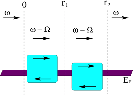
Figure 6: (Color online) Third-order process describing creation of a pair by initial electron at point ${\bf r}=0$, rescattering within the pair at point ${\bf r}={\bf r}_{1}$, and annihilation of the pair at point ${\bf r}={\bf r}_{2}$. Diagram corresponding to this process is shown later in the text (first diagram in Fig. 8).

We start with a three-scattering process in the regime of arcs, and demonstrate qualitatively how the frequency scale, $v_{\text{\tiny F}}/r_{\text{\tiny I}}$, emerges. Three-scattering process involves two virtual pairs. Consider first this process in the absence of the random field. It is illustrated in Fig. 6. In analysis of this process suhas1 ; suhas2 ; suhas3 it was established that the directions of momenta of the participating electrons are strongly correlated, namely, they are either almost parallel or almost antiparallel. Quantitative estimate for the degree of alignment of the momenta can be obtained from inspection of Fig. 6. If the scattering acts take place at points $0$, ${\bf r}_{1}$, and ${\bf r}_{2}$, then the corresponding matrix element contains a phase factor

$$\exp\left[2ik_{\text{\tiny F}}\left(r_{1}-r_{2}+|{\bf r}_{1}-{\bf r}_{2}|\right)\right].$$ (68)

This phase factor does not oscillate, if the angle between the vectors ${\bf r}_{1}$ and ${\bf r}_{2}$ is smaller than $\left(1/k_{\text{\tiny F}}r\right)^{1/2}$, where $r$ is the typical length of ${\bf r}_{1}$, ${\bf r}_{2}$.

The above angular restriction constitutes the origin of a zero-bias anomaly in the regime of arcs. Zero-bias anomaly emerges as a result of the suppression of the three-scattering process in the field, $h_{0}$. This suppression is due to curving of the electron trajectory by the angle $\sim r/R_{\text{\tiny L}}$, see Fig. 5, and it occurs when the curving angle exceeds the allowed angle of alignment. Therefore, upon equating $\left(1/k_{\text{\tiny F}}r\right)^{1/2}$ to $r/R_{\text{\tiny L}}$, we find $r=r_{\text{\tiny I}}$, which leads us to the conclusion that $\omega\sim v_{\text{\tiny F}}/r_{\text{\tiny I}}$ is the energy scale at which $\delta\nu(\omega)$ exhibits a feature. Note that, in considering the Friedel oscillations, we inferred the scale $r_{\text{\tiny I}}$ from a different condition, namely, that the additional phase, $\sim(p_{0}r_{\text{\tiny I}})^{3}$, due to the elongation of a trajectory in magnetic field is $\lesssim 1$. Thus we conclude that, in the regime of arcs, the same spatial scale, $r_{\text{\tiny I}}$, which governs the “dephasing” of $\Pi_{2k_{\text{\tiny{F}}}}(r)$ (a polarization bubble) also governs the suppression of the three-scattering process, which involves three loops .

The above analysis of phases in the matrix element of the three-scattering process can be extended to the regime of snakes. This analysis yields that three-scattering process is efficient at distances $r\lesssim r_{\text{\tiny II}}$, see Eq. (11). Analysis of phases similar to the phase, given by Eq. (68), also suggests that two-scattering processes are insensitive to the magnetic field. This insensitivity can be explained as follows. Calculation of the contribution to the density of states from the three-scattering process with matrix element Eq. (68) involves integration over positions of ${\bf r}_{1}$ and ${\bf r}_{2}$, with respect to the origin, ${\bf r}=0$, which reveals the angular restriction on their orientations. Similar integration for a two-scattering process involves only the orientation of the interaction point, ${\bf r}$, with respect to the origin. Then the angular restriction, and its lifting by magnetic field, does not emerge. In the next subsection the above qualitative arguments are supported by a rigorous calculation.

VII Density of states: Analytical derivation

VII.1 Absence of a zero-bias anomaly in the second order in the interaction strength

Figure 7: Diagrams for the second-order corrections Eq. (70) (left) and Eq. (VII.1) (right) to the density of states.

We start from general expression for the average density of states

$$\delta\nu(\omega)=-\frac{1}{\pi}\;\Bigl{\langle}{\text{Im}}\;G_{\omega}({\bf r},{\bf r})\Bigr{\rangle}_{h(x,y)},$$ (69)

where $\langle\dots\rangle$ denotes disorder averaging defined by Eq. (V.2.2). In the second order in interaction strength, the random-field-induced correction to the density of states are determined by two diagrams shown in Fig. 7. The corresponding analytical expressions read

$$\delta\nu_{1}(\omega)\! = \!4\;{\text{Im}}\frac{2}{\pi}\int\frac{d\Omega}{2\pi}\int d{\bf r}\;d{\bf r}_{1}d{\bf r}_{2}\;G_{\omega}({\bf r},{\bf r}_{1})$$ (70)

$$\times \!G_{\Omega}({\bf r}_{1},{\bf r}_{2})\Bigl{\{}V^{2}\!\left(2k_{\text{\tiny F}}\right)\Pi_{2k_{\text{\tiny{F}}}}({\bf r}_{1},{\bf r}_{2},\omega-\Omega)$$

$$+ \!V^{2}(0)\Pi_{0}({\bf r}_{1},{\bf r}_{2},\omega-\Omega)\Bigr{\}}G_{\omega}({\bf r}_{2},{\bf r}),$$

$$\delta\nu_{2}(\omega)\!\! = \!\!-2\;{\text{Im}}\frac{2}{\pi}\int\frac{d\Omega}{2\pi}\int d{\bf r}\;d{\bf r}_{1}d{\bf r}_{2}\;G_{\omega}({\bf r},{\bf r}_{1})$$

$$\times \!\!G_{\Omega}({\bf r}_{1},{\bf r}_{2})G_{\omega}({\bf r}_{2},{\bf r})\Bigl{\{}V(0)\bigl{[}2V(2k_{\text{\tiny F}})-V(0)\bigr{]}$$

$$\times \!\!\!\Pi_{2k_{\text{\tiny{F}}}}({\bf r}_{1},{\bf r}_{2},\omega-\Omega)+V^{2}(0)\Pi_{0}({\bf r}_{1},{\bf r}_{2},\omega-\Omega)\Bigr{\}},$$

where $V(0)$ and $V(2k_{\text{\tiny F}})$ are the Fourier components of the interaction potential $V({\bf r})$ with momenta zero and $2k_{\text{\tiny F}}$, respectively. Three Green functions in Eqs. (70), (VII.1) describe the propagation of electron between the points $\left({\bf r},{\bf r}_{1}\right)$, $\left({\bf r}_{1},{\bf r}_{2}\right)$, and $\left({\bf r}_{2},{\bf r}\right)$, Fig. 7 . Polarization bubble describes the creation of electron-hole pair at point ${\bf r}_{1}$ and annihilation at point ${\bf r}_{2}$. Difference in signs in Eqs.  (70), (VII.1) is due to the fact that the first diagram contains two closed fermionic loops, whereas the second diagram contains only one. Numerical factors $4$ and $2$ in Eqs. (70), (VII.1) come from summation over the spin indices. The difference between them is due two the fact the spin of electron-hole pair is not fixed in the first diagram, but it is fixed in the second diagram. The factor $2$ in the product $2V(0)V(2k_{\text{\tiny F}})$ in Eq. (VII.1) is related to the annihilation of the electron-hole pair, since the hole is annihilated with initial electron. Then the momentum transfer can be $2k_{\text{\tiny F}}$ in the course of creation and zero in the course of annihilation, and vice versa.

Figure 8: Third-order diagrams contributing to the zero-bias anomaly in the density of states. Random field enters via the phases of the Green functions.

It is important to emphasize that the Green functions and polarization operators in Eqs. (70), (VII.1) contain the information about the random field, $h(x,y)$, via their additional phases: $\varphi_{{\bf r}_{1}\rightarrow{\bf r}_{2}}$ in $G_{\omega}({\bf r}_{1},{\bf r}_{2})$ and $2\varphi_{{\bf r}_{1}\rightarrow{\bf r}_{2}}$ in $\Pi_{2k_{\text{\tiny{F}}}}({\bf r}_{1},{\bf r}_{2},\omega)$. The phase, $\varphi_{{\bf r}_{1}\rightarrow{\bf r}_{2}}$, always enters in combination with a main term, $k_{\text{\tiny F}}|{\bf r}_{1}-{\bf r}_{2}|$. Obviously, $\Pi_{0}({\bf r}_{1},{\bf r}_{2},\omega)$ does not contain a field-induced phase. Thus, only the terms containing $\Pi_{2k_{\text{\tiny{F}}}}$ in Eqs. (70), (VII.1) should be considered.

Now it is easy to see that $\delta\nu_{1}$ and $\delta\nu_{2}$ do not exhibit a field-induced anomaly at small $\omega$. This is because the field dependence is cancelled out in the integrands of Eqs. (70), (VII.1). To see this, we first note that the integration over ${\bf r}$ in Eqs. (70), (VII.1) can be easily performed using the fact that $\int d{\bf r}G_{\omega}({\bf r}_{1},{\bf r})G_{\omega}({\bf r},{\bf r}_{2})$ is equal to the derivative, $\partial G_{\omega}({\bf r}_{1},{\bf r}_{2})/\partial\omega$. Then we note that the contribution to $\delta\nu_{1}$, $\delta\nu_{2}$ comes only from “slow” terms, in the product of two Green functions, $G_{\omega}({\bf r}_{1},{\bf r}_{2})$, $G_{\Omega}({\bf r}_{1},{\bf r}_{2})$, and $\Pi_{2k_{\text{\tiny{F}}}}$. These slow terms do not contain rapidly oscillating factors $\exp\{2ik_{\text{\tiny F}}|{\bf r}_{1}-{\bf r}_{2}|\}$. On the other hand, cancellation of the rapid terms in the product automatically results in the cancellation of the field-dependent terms.

As it was explained in qualitative discussion, the situation changes in the third order in the interactions. Corresponding expression for $\delta\nu(\omega)$ is derived in the next Subsection.

VII.2 General expression for the third-order interaction correction to the density of states.

Relevant diagrams for the third-order correction to the density of states are shown in Fig. 8. The same 8 diagrams were considered in Ref. suhas3, in the momentum space. In Ref. suhas3, the analysis of these diagrams was restricted to small momenta. In our coordinate representation this means that only $\Pi_{0}({\bf r})$ parts of the polarization operators was kept, whereas $\Pi_{2k_{\text{\tiny{F}}}}({\bf r})$ parts were neglected. As explained above, to reveal the sensitivity to the random field, we will keep only the $\Pi_{2k_{\text{\tiny{F}}}}({\bf r})$ parts. Then the correction to the Green function corresponding to the sum of eight diagrams in Fig. 8 acquires the form

$$\delta \!\!\!\!\nu(\omega)=2V(0)V(2k_{\text{\tiny F}})\Bigl{[}2V(2k_{\text{\tiny F}})-V(0)\Bigr{]}$$

$$\times {\text{Im}}\frac{i}{2\pi^{2}}\int\frac{d\Omega}{2\pi}\int d{\bf r}\;d{\bf r}_{1}d{\bf r}_{2}\;G_{\omega}({\bf r},{\bf r}_{1})\;G_{\Omega}({\bf r}_{1},{\bf r}_{2})$$

$$\times \Pi_{2k_{\text{\tiny{F}}}}({\bf r}_{1},0,\omega-\Omega)\;\Pi_{2k_{\text{\tiny{F}}}}(0,{\bf r}_{2},\omega-\Omega)\;G_{\omega}({\bf r}_{2},{\bf r}).$$

All the diagrams reduce to the same integrals. Concerning the difference in numerical coefficients, it comes from the number of closed fermionic loops and the spin degrees of freedom. Taking this into account interaction coefficient corresponding to the first two diagrams will be $2\cdot(-2)^{2}V^{3}(2k_{\text{\tiny{F}}})$. Coefficient of the third diagram is $(-2)^{3}V^{3}(2k_{\text{\tiny{F}}})$. Thus we see, that the contributions $\propto V^{3}(2k_{\text{\tiny{F}}})$ cancel each other.

The first and the second diagrams in the second row are equal to each other, and each of them has a coefficient $(-2)^{2}V(0)V^{2}(2k_{\text{\tiny{F}}})$. Coefficient of the last diagram in the second row is $(-2)V^{2}(0)V(2k_{\text{\tiny{F}}})$, since it has only one closed fermionic loop. Finally, the first diagram in third row has only one closed fermionic loop and is equal to the second diagram on the third row. Each of these diagrams contributes with the coefficient $(-2)V(0)V^{2}(2k_{\text{\tiny{F}}})$.

On the physical level, 8 diagrams in Fig. 8 describe different electron-electron three-scattering processes. For example, the first diagram corresponds to creation of electron-hole pair by the initial electron followed by rescattering within a created pair and, finally, its annihilation. Three stages of this process are illustrated in Fig. 6. However, creation, rescattering, and annihilation of a pair can follow a different scenario, namely, the rescattering process can involve the initial electron. This scenario is captured by the second diagram in the first row in Fig. 8.

Figure 9: (a) Eight diagrams for $\delta G_{\omega}({\bf r},{\bf r})$, that are shown in Fig. 8, are combined into one generalized diagram. Electron-electron scattering processes take place at points $0$, ${\bf r}_{1}$, and ${\bf r}_{2}$; (b) Eight third-order diagrams that do not contribute to the zero-bias anomaly are combined into one generalized diagram; (c) Two types of four-leg interaction vertices are combined into big dots; (d) An example of a third-order diagram of type (b).

At this point, we note that diagrams in Fig. 8 do not exhaust all possible three-scattering processes. In fact, all diagrams in Fig. 8 have identical structure, in the sense, that they can be combined into a single generalized diagram, as shown in Fig. 9a. There are also eight other diagrams combined into a single generalized diagram, as shown in Fig. 9b that are not sensitive to the random field. This is because, in the absence of the random field, the phase factor corresponding to Fig. 9b is large, namely, $2\cdot 2k_{\text{\tiny{F}}}(r_{1}+r_{2})$.

The crucial difference between the contributions Eqs. (70), (VII.1) and Eq. (VII.2) is that the cancellation of the rapid-oscillating terms in in the integrand of Eq. (VII.2) preserves the field-dependence. To see this, we first replace $\int d{\bf r}G_{\Omega}({\bf r}_{1},{\bf r})G_{\Omega}({\bf r},{\bf r}_{2})$ by $\partial G_{\Omega}({\bf r}_{1},{\bf r}_{2})/\partial\Omega$, as discussed above, and then consider the phase of the product

$$G_{\Omega}({\bf r}_{1},{\bf r}_{2})~{}G_{\omega}({\bf r}_{1},{\bf r}_{2})\qquad\qquad\qquad\qquad\qquad$$

$$\times\Pi_{2k_{\text{\tiny{F}}}}(0,{\bf r}_{2},\omega-\Omega)~{}\Pi_{2k_{\text{\tiny{F}}}}({\bf r}_{1},0,\omega-\Omega).$$ (73)

Fig. 5b illustrates this product graphically. It is seen from Fig. 5b that, when the fast oscillating terms $\exp\{2ik_{\text{\tiny F}}|{\bf r}_{1}-{\bf r}_{2}|\}$, $\exp\{2ik_{\text{\tiny F}}r_{1}\}$, and $\exp\{2ik_{\text{\tiny F}}r_{2}\}$ cancel each other out, the additional phase enters into the product either in combination

$$2\delta\varphi_{\Sigma}^{(+)}=2\delta\varphi_{{\bf r}_{1}\rightarrow 0}+2\delta\varphi_{{\bf r}_{2}\rightarrow 0}-2\delta\varphi_{{\bf r}_{1}\rightarrow{\bf r}_{2}},$$ (74)

or in combination (see Fig. 5b)

$$2\delta\varphi_{\Sigma}^{(-)}=2\delta\varphi_{{\bf r}_{1}\rightarrow 0}-2\delta\varphi_{{\bf r}_{2}\rightarrow 0}+2\delta\varphi_{{\bf r}_{1}\rightarrow{\bf r}_{2}}.$$ (75)

Since additional phases defined by Eqs. (33), (34) are cubic in distance, the combinations Eq. (74) and Eq. (75) are nonzero. This is in contrast to the two-scattering processes, where the cancellation occurs identically for arbitrary dependence of $\delta\varphi(r)$ on $r$. In turn, non-cancellation of additional phases in Eqs. (74), (75) means that the random field causes a zero-bias anomaly, more specifically, a feature in $\delta\nu(\omega)$ at small $\omega$.

The final form of $\delta\nu(\omega)$ emerges upon integration of Eq. (VII.2) over azimuthal angles of ${\bf r}_{1}$ and ${\bf r}_{2}$, which can be performed analytically, using the relation

$$\left\langle e^{i{\bf p}\left({\bf r}_{1}+{\bf r}_{2}\right)}\right\rangle_{\varphi_{\bf p},\varphi_{{\bf r}_{1}},\varphi_{{\bf r}_{2}}}=\frac{\sin\left[p\left(r_{1}\pm r_{2}\right)+\pi/4\right]}{p(r_{1}r_{2})^{1/2}}.$$ (76)

Upon combining rapidly oscillating terms in the integrand of Eq. (VII.2) into “slow” terms, we obtain

$$\delta\nu(\omega)=\delta\nu^{(+)}(\omega)+\delta\nu^{(-)}(\omega),$$ (77)

where

$$\frac{\delta\nu^{(+)}(\omega)}{\nu_{0}}=-\frac{(\nu_{0}V)^{3}}{2E_{\text{\tiny F}}\pi^{3/2}k_{\text{\tiny F}}^{1/2}}\!\int_{r_{2}>r_{1}}\frac{d{r_{1}}d{r_{2}}}{(r_{1}r_{2})^{3/2}}$$

$$\times(r_{1}+r_{2})^{1/2}\int_{0}^{\omega}\!\!d\Omega\sin\left[v_{\text{\tiny F}}^{-1}(\omega-\Omega)(r_{1}+r_{2})\right]$$

$$\times\sin\left\{2\delta\varphi_{\Sigma}^{(+)}+\frac{\pi}{4}-\frac{(\omega+\Omega)}{v_{\text{\tiny F}}}(r_{1}+r_{2})\right\},$$ (78)

and

$$\frac{\delta\nu^{(-)}(\omega)}{\nu_{0}}=-\frac{(\nu_{0}V)^{3}}{2E_{\text{\tiny F}}\pi^{3/2}k_{\text{\tiny F}}^{1/2}}\!\int_{r_{2}>r_{1}}\frac{d{r_{1}}d{r_{2}}}{(r_{1}r_{2})^{3/2}}$$

$$\times(r_{2}-r_{1})^{1/2}\int_{0}^{\omega}\!\!d\Omega\sin\left[v_{\text{\tiny F}}^{-1}(\omega-\Omega)(r_{1}+r_{2})\right]$$

$$\times\sin\left\{2\delta\varphi_{\Sigma}^{(-)}+\frac{\pi}{4}+\frac{(\omega+\Omega)}{v_{\text{\tiny F}}}(r_{2}-r_{1})\right\},$$ (79)

where we had assumed that the interaction is short-ranged and set $V(0)=V(2k_{\text{\tiny F}})=\nu_{0}V$. Two contributions in Eq. (77) correspond to the locations of the points ${\bf r}_{1}$ and ${\bf r}_{2}$ on the opposite and the same sides from the origin, respectively, see Fig. 5b.

We note that the phases $\delta\varphi_{\Sigma}^{(+)}$, $\delta\varphi_{\Sigma}^{(-)}$, which enter into the argument of sine in Eqs. (VII.2), (VII.2), are quadratic in the random field, $h(x,y)$, as seen from Eqs. (33), (34). This suggests that the averaging over realizations of $h(x,y)$ can be carried out analytically in the integrands of Eqs. (VII.2), (VII.2). Similarly to the case of Friedel oscillations, it is convenient to perform this averaging separately for the regimes I and II. This is done in Sections VIII, IX below. In the remainder of this Section we will evaluate the interaction correction, $\delta\nu(\omega)$, for two particular cases: (i) constant magnetic field, $h(x,y)\equiv h_{0}$, in a clean electron gas, and (ii) $h(x,y)\equiv h_{0}$ in electron gas with small concentration of point-like impurities.

VII.3 Case of Constant Magnetic Field: Oscillations of $\delta\nu(\omega)$

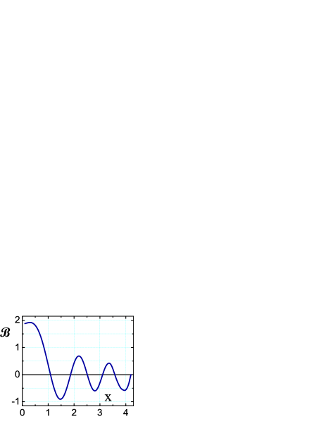
Figure 10: (Color online) Dimensionless correction Eq. (81) to the tunnel density of states in a weak constant magnetic field is plotted vs. dimensionless energy $x=2^{2/3}\omega/\omega_{0}$. The plot is obtained upon numerical integration in Eqs. (VII.2), (VII.2).

In a constant magnetic field $h(x,y)\equiv h_{0}$ the characteristic scale of frequency in Eqs. (VII.2), (VII.2) is $\omega_{0}=v_{\text{\tiny F}}/r_{\text{\tiny I}}$. This was stated in Section III. Now this scale of frequencies emerges naturally upon substituting in Eqs. (VII.2), (VII.2) the phases $2\delta\varphi_{\Sigma}^{(+)}$, $2\delta\varphi_{\Sigma}^{(+)}$, calculated from Eq. (33) in a constant magnetic field

$$2\delta\varphi_{\Sigma}^{(\pm)}=\mp\frac{p_{0}^{3}}{4}r_{1}r_{2}(r_{1}\pm r_{2}),$$ (80)

where $p_{0}$ is defined by Eq. (4). The integrals in Eqs. (VII.2), (VII.2) converge at distances $r_{1},r_{2}\sim p_{0}^{-1}=r_{\text{\tiny I}}$. As a result, $\delta\nu^{(+)}$ and $\delta\nu^{(-)}$ are certain universal functions of $\omega r_{\text{\tiny I}}/v_{\text{\tiny F}}=\omega/\omega_{0}$. The plot of $\delta\nu^{(+)}+\delta\nu^{(-)}$ vs. dimensionless ratio $x=2^{2/3}\omega/\omega_{0}$ is presented in Fig. 10. To isolate the frequency dependence, in addition to $x$, we had introduced the dimensionless variables $r_{1}/r_{\text{\tiny I}}$ and $r_{2}/r_{\text{\tiny I}}$ after which $\delta\nu(\omega)$ acquires the form

$$\frac{\delta\nu(\omega)}{\nu_{0}}=-\frac{(\nu_{0}V)^{3}}{2^{2/3}(\pi k_{\text{\tiny F}}r_{\text{\tiny I}})^{3/2}}{\mathcal{B}}(x).$$ (81)

The integral over $\Omega$ in Eqs. (VII.2), (VII.2) can be evaluated analytically. The remaining dimensionless double integrals were calculated numerically. While the characteristic scale, $x\sim 1$, of change of the function ${\mathcal{B}}(x)$ follows from qualitative consideration, Fig. 10 indicates that ${\mathcal{B}}(x)$ also exhibits sizable oscillations. These oscillations come only from the contribution $\delta\nu^{(+)}$. They owe their existence to the peculiar structure of the argument of sine in Eq. (VII.2). Namely, this argument has saddle points with respect to both $r_{1}$ and $r_{2}$ at $r_{1}=r_{2}=2^{1/3}r_{\text{\tiny I}}(\omega/\omega_{0})^{1/2}/3^{1/2}$ Oscillatory behavior of ${\mathcal{B}}(x)$ is governed by the value of the argument at the saddle point, which is $\sim(\omega/\omega_{0})^{3/2}$. Strictly speaking, the saddle point determines the value of the integral only when $\omega\gg\omega_{0}$. However, numerics shows that oscillations in Fig. 10, set in starting already from $x\sim 1$. These oscillations reflect the distinguished contribution from the three-scattering process, shown in Fig. 5b, in which scattering events occur at $r_{1}=r_{2}=2^{1/3}r_{\text{\tiny I}}(\omega/\omega_{0})^{1/2}/3^{1/2}$.

Eq. (81) and Fig. 10 constitute an experimentally verifiable prediction. Correction Eq. (81) describes the the feature in the tunneling conductance of a clean two-dimensional electron gas as a function of bias that emerges in a weak magnetic field, $h_{0}$. It follows from prefactor in Eq. (81) that the magnitude of $\delta\nu$ scales with $h_{0}$ as $r_{\text{\tiny I}}^{-3/2}\propto h_{0}$. We emphasize that the correction $\delta\nu(\omega)$ remains distinguishable even when the structure in the density of states due to the Landau quantization is completely smeared out, e.g., due to finite temperature. This follows from the above relation between $\omega_{0}$ and the cyclotron frequency, $\omega_{c}$, namely, $\left(\omega_{c}/\omega_{0}\right)\sim\left(\omega_{c}/E_{\text{\tiny F}}\right)^{1/3}\ll 1$.

In discussing the relevance to the experiment one should have in mind that realistic samples always contain certain degree of disorder. Therefore, the question remains as to whether the oscillations of $\delta\nu(\omega)$ in a constant magnetic field survive in the presence of the short-range impurities. This question is non-trivial, since impurities themselves give rise to the singular correction to $\delta\nu(\omega)$ (zero-bias anomaly) even in a zero field. Then the above question can be reformulated as: whether the field-induced oscillations are distinguishable on the background of a zero-bias anomaly. It turns out that, by introducing the Friedel oscillations, point-like impurities actually enhance the oscillatory part of $\delta\nu(\omega)$. This question is addressed in the next subsection.

Figure 11: Second-order diagrams contributing to the oscillating part (see Fig. 4) of the ballistic zero-bias anomaly in a weak constant magnetic field. Magnetic field enters through the phases Eq. (22) of the Green functions. Dashed line represents the impurity scattering. All $12$ diagrams (a)-(l) contain two static polarization operators.

VII.4 Ballistic Zero-Bias Anomaly in a Constant Magnetic Field

Conventional ballistic zero-bias anomalyrudin97 , caused by point-like impurities, is described by two second-order diagrams, shown Fig. 7, in which one of two interaction lines is replaced by an impurity line. As was shown in Ref. rudin97, , these diagrams with one interaction line and one impurity line yield a singular correction, $\delta\nu(\omega)/\nu_{0}\sim\left(\nu_{0}V/E_{\text{\tiny F}}\tau\right)\ln(\omega)$, to the density of states. Here $\tau^{-1}$ is the scattering rate proportional to the impurity concentration. Qualitatively, the singular correction originates from the combined scattering of electron by the impurity and the Friedel oscillation $\propto\sin(2k_{\text{\tiny F}}r)/r^{2}$, created by the same impurity. This Friedel oscillation is represented by the polarization loop in Fig. 7. In the presence of the impurity, this loop describes static response of the electron gas, and thus the polarization operator, $\Pi_{2k_{\text{\tiny F}}}(\omega,r)$, corresponding to the loop should be taken at $\omega=0$. As was mentioned in Section III, a weak perpendicular magnetic field, $h$, leaves the logarithmic correction unchanged. To reveal the sensitivity to $h$, one should calculate $\delta\nu$ to the next (second) order in $V$. Corresponding diagrams with one impurity and two interaction lines are shown in Figs. 11, 12, and 13. It is easy to see that there are overall $24$ different diagrams. Indeed, the generalized diagram, Fig. 9(a), for the third-order interaction correction contains three generalized four-leg vertices shown in Fig. 9(c). Hence, Fig. 9 (a) represents $2^{3}=8$ different diagrams. In each of these $8$ diagrams, the impurity line can replace interaction line in three places, generating one of $24$ different diagrams that are shown in Figs. 11, 12, and 13. All these diagrams are divided into three groups according to their dependence on $\omega$. Namely, all $12$ diagrams in Fig. 11 have the same $\omega$-dependence. Similarly, the $\omega$-dependence of all $8$ diagrams in Fig. 12 is the same. This also applies to $4$ diagrams in Fig. 13. However, the corresponding $\omega$-dependencies are slightly different from each other. The origin of this difference can be traced from comparison of diagrams Fig. 11 (a), Fig. 12 (a), and Fig. 13 (b). Diagram Fig. 11 (a) contains two polarization loops separated by the impurity line. As a result, the expression corresponding to this diagram, contains two static polarization operators, $\Pi_{2k_{\text{\tiny F}}}(0,r)$. Diagram Fig. 12 (a) contains one finite-$\omega$ polarization loop, $\Pi_{2k_{\text{\tiny F}}}(\omega,r)$. Finally, the diagram Fig. 13 (b) does not contain polarization operators at all, but rather a different object, namely, a polarization loop crossed by the impurity line. Important is that the expression, corresponding to this object

$$\!\!\!\!\!\!\!\!\!\!\!\!{\prod}(\omega-\Omega,|{\bf r}_{1}-{\bf r}_{2}|)=-i\int\frac{d\Omega_{1}}{2\pi}G_{\Omega_{1}}(0,{\bf r}_{1})$$

$$\!\!\!\!\!\!\!\!\!\!\!\!\!\times G_{\omega-\Omega+\Omega_{1}}({\bf r}_{1},0)G_{\omega-\Omega+\Omega_{1}}(0,{\bf r}_{2})G_{\Omega_{1}}({\bf r}_{2},0),$$ (82)

contains a “fast” part, ${\prod}_{2k_{\text{\tiny F}}}(\omega,r)$, which oscillates as $\exp\left(2ik_{\text{\tiny F}}|{\bf r}_{1}-{\bf r}_{2}|\right)$, i.e., in the same way as polarization operator.

Figure 12: $8$ out of total $24$ second-order diagrams for ballistic zero-bias anomaly in a weak constant magnetic field, which contain one dynamic polarization operator.

The full analytical expression corresponding to the diagram Fig. 11 (a) reads

$$\delta\nu_{1}(\omega,h)={\text{Im}}\frac{4V^{2}(2k_{\text{\tiny F}})}{2\pi^{2}\nu_{0}\tau}\int d{\bf r}d{\bf r}_{1}d{\bf r}_{2}\;G_{\omega}({\bf r},{\bf r}_{1})$$

$$\times G_{\omega}({\bf r}_{1},{\bf r}_{2})\Pi_{2k_{\text{\tiny F}}}(0,{\bf r}_{1})\Pi_{2k_{\text{\tiny F}}}(0,{\bf r}_{2})G_{\omega}({\bf r}_{2},{\bf r})$$

$$={\text{Im}}\frac{6V^{2}(2k_{\text{\tiny F}})}{\pi^{2}\nu_{0}\tau}\int d{\bf r}_{1}\;d{\bf r}_{2}\;\partial_{\omega}G_{\omega}({\bf r}_{1},{\bf r}_{2})$$

$$\times G_{\omega}({\bf r}_{1},{\bf r}_{2})\Pi_{2k_{\text{\tiny F}}}(0,{\bf r}_{1})\Pi_{2k_{\text{\tiny F}}}(0,{\bf r}_{2}),$$ (83)

where in the second identity we had performed integration over ${\bf r}$.

Analytical expression for the diagram Fig. 12 (a) has the form

$$\delta\nu_{2}(\omega,h)=-{\text{Im}}\frac{2V^{2}(2k_{\text{\tiny F}})}{2\pi^{2}\nu_{0}\tau}\!\!\int\!\!d{\bf r}\;d{\bf r}_{1}d{\bf r}_{2}$$

$$\times\;G_{\omega}({\bf r},{\bf r}_{1})G_{\omega}({\bf r}_{1},0)G_{\omega}({\bf r}_{2},{\bf r})$$ (84)

$$\times\int\frac{d\Omega}{2\pi}G_{\Omega}(0,{\bf r}_{1})G_{\Omega}({\bf r}_{1},{\bf r}_{2})\Pi_{2k_{\text{\tiny F}}}(\omega-\Omega,|{\bf r}_{1}-{\bf r}_{2}|).$$

Finally, the expression for the diagram 13 (b) is the following

$$\!\!\!\!\!\!\!\delta\nu_{3}(\omega,h)=-{\text{Im}}\frac{2V^{2}(2k_{\text{\tiny F}})}{2\pi^{2}\nu_{0}\tau}\!\!\int\!\!d{\bf r}\;d{\bf r}_{1}d{\bf r}_{2}\;G_{\omega}({\bf r},{\bf r}_{1})G_{\omega}({\bf r}_{2},{\bf r})$$

$$\times\int\frac{d\Omega}{2\pi}\int\frac{d\Omega_{1}}{2\pi}G_{\Omega}({\bf r}_{1},{\bf r}_{2})G_{\Omega_{1}}(0,{\bf r}_{1})$$

$$\times G_{\omega-\Omega+\Omega_{1}}({\bf r}_{1},0)G_{\omega-\Omega+\Omega_{1}}(0,{\bf r}_{2})G_{\Omega_{1}}({\bf r}_{2},0).$$ (85)

Upon integration over ${\bf r}$, it can be expressed through ${\prod}_{2k_{\text{\tiny F}}}(r)$, defined by Eq. (VII.4), as

$$\!\!\!\!\!\!\!\delta\nu_{3}(\omega,h)=-\frac{V^{2}(2k_{\text{\tiny F}})}{\pi^{4}\nu_{0}\tau}\!\!\int\!\!d{\bf r}_{1}d{\bf r}_{2}\;\partial_{\omega}{\text{Im}}G_{\omega}({\bf r}_{1},{\bf r}_{2})$$

$$\times\int_{0}^{\omega}\frac{d\Omega}{2\pi}{\text{Im}}G_{\Omega}({\bf r}_{1},{\bf r}_{2}){\text{Im}}\;{\prod}_{2k_{\text{\tiny F}}}(\omega-\Omega,|{\bf r}_{1}-{\bf r}_{2}|).$$

Figure 13: $4$ out of total $24$ second-order diagrams for the ballistic zero-bias anomaly in a weak constant magnetic field, which contain a polarization loop crossed by the impurity line.

Despite all $12$ diagrams in Fig. 11 have the same frequency dependence, their prefactors represent different combinations of $V^{2}(2k_{\text{\tiny F}})$, $V^{2}(0)$, and $V(2k_{\text{\tiny F}})V(0)$. The same applies to $8$ diagrams in Fig. 12 and to $4$ diagrams in Fig. 13. Taking into account the numerical factors in these combinations amounts to the following replacements: in $\delta\nu_{1}$

$$4V^{2}(2k_{\text{\tiny F}})\rightarrow 3V^{2}(0),$$ (87)

in $\delta\nu_{2}$

$$-2V^{2}(2k_{\text{\tiny F}})\rightarrow 4\Bigl{[}V(0)V(2k_{\text{\tiny F}})-V^{2}(2k_{\text{\tiny F}})-V^{2}(0)\Bigr{]},$$

and in $\delta\nu_{3}$

$$-2V^{2}(2k_{\text{\tiny F}})\rightarrow 2\Bigl{[}V(0)V(2k_{\text{\tiny F}})-V^{2}(2k_{\text{\tiny F}})-V^{2}(0)\Bigr{]}.$$

These replacements must be taken into account when calculating the full correction $\delta\nu(\omega)$ from $\delta\nu_{1}$, $\delta\nu_{2}$, and $\delta\nu_{3}$.

Below we demonstrate that all three contributions $\delta\nu_{1}$, $\delta\nu_{2}$, and $\delta\nu_{3}$ are oscillatory functions of $\omega$. Detailed derivation will be presented only for $\delta\nu_{1}$.

Analogously to the derivation of Eqs. (VII.2), (VII.2), we can perform the integration over the azimuthal angles of ${\bf r}_{1}$ and ${\bf r}_{2}$ analytically using Eq. (76). Then, extracting a “slow” term from the product of trigonometrical functions, we obtain $\delta\nu_{1}(\omega)=\left[{6\nu_{0}^{3}V^{2}(2k_{\text{\tiny F}})}/{E_{\text{\tiny F}}\tau}\right]\left(\omega_{0}/E_{\text{\tiny F}}\right)^{1/2}\text{\large P}_{1}(2^{2/3}\omega/\omega_{0})$, with $\omega_{0}=2^{1/3}\omega_{c}^{2/3}E_{\text{\tiny F}}^{1/3}$, where the function $\text{\large P}_{1}(x)$ is defined as

$$\text{\large P}_{1}(x)=\text{\large P}^{+}_{1}(x)+\text{\large P}^{-}_{1}(x),$$ (90)

where

$$\text{\large P}^{+}_{1}(x)=\sigma\int_{\rho_{2}>\rho_{1}}\frac{d\rho_{1}d\rho_{2}}{(\rho_{1}\rho_{2})^{3/2}}\Biggl{\{}(\rho_{1}+\rho_{2})^{1/2}$$

$$\times\Bigl{\{}\cos\left[x(\rho_{1}+\rho_{2})-\frac{\pi}{4}-\rho_{1}\rho_{2}(\rho_{1}+\rho_{2})\right]$$

$$-\cos\left[x(\rho_{1}+\rho_{2})-\frac{\pi}{4}\right]\Bigr{\}}\Biggr{\}},$$ (91)

$$\text{\large P}^{-}_{1}(x)=-\sigma\int_{\rho_{2}>\rho_{1}}\frac{d\rho_{1}d\rho_{2}}{(\rho_{1}\rho_{2})^{3/2}}\Biggl{\{}(\rho_{2}-\rho_{1})^{1/2}$$

$$\times\Bigl{\{}\cos\left[x(\rho_{2}-\rho_{1})+\frac{\pi}{4}+\rho_{1}\rho_{2}(\rho_{2}-\rho_{1})\right]$$

$$-\cos\left[x(\rho_{2}-\rho_{1})+\frac{\pi}{4}\right]\Bigr{\}}\Biggr{\}}.$$ (92)

Here the constant factor, $\sigma$, is given by $\sigma=(3\cdot 2^{1/6})/\pi^{3/2}$. In Appendix E we demonstrate how the function $\text{\large P}_{1}(x)$ can be cast in the form that is convenient for numerical evaluation and extracting asymptotes. This form is given by the following double integral

$$\text{\large P}_{1}(x)=4\sigma\int_{0}^{\infty}\frac{dz}{z^{3/2}}\int_{-4}^{0}\frac{dv}{\sqrt{v+4}}\qquad\qquad$$ (93)

$$\times\Biggl{(}\cos\left[xz+\frac{\pi}{4}+\frac{z^{3}}{v}\right]-\cos\left[xz+\frac{\pi}{4}\right]\Biggr{)}.$$

The fact that $\text{\large P}_{1}(x)$ oscillates at large $x\gg 1$ follows from the observations that (i) first cosine in the brackets in Eq. (93) has a saddle point $z=(x|v|/3)^{1/2}$, and (ii) the major contribution to the integral over $v$ comes from the lower limit $v=-4$ (corresponding steps are outlined in Appendix D). This yields

$$\text{\large P}_{1}(x)\mbox{\Large$|$}_{x\gg 1}=\frac{2^{5/3}3^{9/4}}{\pi^{1/2}}\;\frac{1}{x^{7/4}}\sin\left[4\left(\frac{x}{3}\right)^{3/2}+\frac{\pi}{4}\right].$$

The argument $x^{3/2}$ in the cosine in Eq. (VII.4) can be presented as $\omega^{3/2}/\left(2^{1/2}\omega_{c}E_{\text{\tiny F}}^{1/2}\right)$, so that the “period” in $\omega$ is much bigger than the cyclotron energy, $\omega_{c}$, as was discussed above.

The analysis of the contributions $\delta\nu_{2}(\omega)$ and $\delta\nu_{3}(\omega)$ can be carried out in a similar way. They exhibit the same oscillations as Eq. (VII.4). The difference is that, due to integration over $\Omega$ in Eqs. (VII.4) and (VII.4), both $\delta\nu_{2}(\omega)$ and $\delta\nu_{3}(\omega)$ contain an extra factor $\omega/\omega_{0}$, see Eq.  (15), and thus their contribution to the net correction $\delta\nu$ is dominant at $\omega\gg\omega_{0}$.

VIII Zero-bias anomaly in the averaged density of states in regime I

With the help of the identity Eq. (V.1.1) the integrand in the average $\delta\nu(\omega)$ can be expressed in terms of functions $U_{1,2}\left[r_{1}r_{2}(r_{2}\pm r_{1})p_{0}^{3}/4\right]$, where the functions $U_{1,2}$ are defined as

$$U_{1}(x)=\Biggl{(}\frac{\pi}{2}\Biggr{)}^{1/2}\sqrt{\frac{(1+x^{2})^{1/2}+1}{1+x^{2}}},$$ (95)

$$U_{2}(x)=\Biggl{(}\frac{\pi}{2}\Biggr{)}^{1/2}\sqrt{\frac{(1+x^{2})^{1/2}-1}{1+x^{2}}}.$$ (96)

Upon introducing dimensionless variables $\rho_{1,2}=p_{0}r_{1,2}/2^{2/3}$, we present the final result in the form

$$\frac{\delta\nu(\omega)}{\nu_{0}}={\mathcal{C}}\;{\mathcal{I}}\left(\frac{\omega}{\omega_{0}}\right),$$ (97)

with

$$\omega_{0}=v_{\text{\tiny{F}}}p_{0}=2E_{\text{\tiny{F}}}\left(\frac{h_{0}}{k_{\text{\tiny{F}}}^{2}\Phi_{0}}\right)^{2/3},$$ (98)

and with constant, ${\mathcal{C}}$, defined as

$${\mathcal{C}}=-\frac{(\nu_{0}V)^{3}}{2\pi}\left(\frac{h_{0}}{k_{\text{\tiny{F}}}^{2}\Phi_{0}}\right)=-\frac{(\nu_{0}V)^{3}}{4\sqrt{2}\pi}\left(\frac{\omega_{0}}{E_{\text{\tiny{F}}}}\right)^{3/2}.$$ (99)

The dimensionless function, ${\mathcal{I}}(z)$, describing the shape of the anomaly, is given by the following double integral over $\rho_{1}$, $\rho_{2}$

$${\mathcal{I}}(z)={\mathcal{I}}^{+}(z)+{\mathcal{I}}^{-}(z)\qquad\qquad\qquad\qquad$$ (100)

$$=\int\limits_{\rho_{2}>\rho_{1}}\!\frac{d{\rho_{1}}d{\rho_{2}}}{(\rho_{1}\rho_{2})^{3/2}}\!\!\int\limits_{0}^{z}\!dz^{\prime}\sin\Bigl{[}(z-z^{\prime})(\rho_{1}+\rho_{2})\Bigr{]}\qquad$$

$$\times\Bigl{\{}S_{+}(\rho_{1},\rho_{2})\!+\!C_{+}(\rho_{1},\rho_{2})\!+\!S_{-}(\rho_{1},\rho_{2})\!+\!C_{-}(\rho_{1},\rho_{2})\Bigr{\}},$$

where the functions $S_{+}$, $S_{-}$, $C_{+}$, and $C_{-}$ are defined as

$$S_{\pm}(\rho_{1},\rho_{2})={(\rho_{1}\pm\rho_{2})^{1/2}}\sin\left[\frac{\pi}{4}\mp(z+z^{\prime})(\rho_{1}\pm\rho_{2})\right]$$

$$\times\Biggl{\{}U_{1}\biggl{(}\rho_{1}\rho_{2}(\rho_{1}\pm\rho_{2})\biggr{)}-\sqrt{\pi}\Biggr{\}},\qquad\qquad\qquad\qquad$$ (101)

$$C_{\pm}(\rho_{1},\rho_{2})={(\rho_{1}\pm\rho_{2})^{1/2}}\cos\left[\frac{\pi}{4}\mp(z+z^{\prime})(\rho_{1}\pm\rho_{2})\right]$$

$$\times U_{2}\biggl{(}\rho_{1}\rho_{2}(\rho_{1}\mp\rho_{2})\biggr{)}.\qquad\qquad\qquad\qquad\qquad\qquad$$ (102)

In definitions of $S_{+}$ and $S_{-}$ we had subtracted from the function $U_{1}(\alpha)$ the zero-field value $U_{1}(0)=\sqrt{\pi}$. Integration over $z^{\prime}$ in Eq. (100) can be easily carried out analytically. The remaining integrals over $\rho_{1}$, $\rho_{2}$ were evaluated numerically. Direct numerical integration encounters difficulties due to very fast oscillations of the integrand in Eq. (100). These difficulties can be overcome by a proper change of variables in the integrand. This procedure is described in Appendix D. The resulting shape of the zero-bias anomaly is shown in Fig. 14. The small-$z\ll 1$ behavior of ${\mathcal{I}}(z)$ is $8\ln z$, i.e., it diverges logarithmically. The cutoff is chosen from the condition that ${\mathcal{I}}(z)$ approaches zero at large $z$. Note, that ${\mathcal{I}}(z)$ exhibits a pronounced feature around $z=1$. The origin of this feature lies in strong oscillations of the integrand in Eq. (77). The “trace” of these oscillations survives after averaging over the magnitude of the random field. In fact, the oscillations persist beyond $z=3$. This is reflected in the $z\gg 1$ asymptote of the function ${\mathcal{I}}(z)$,

$${\mathcal{I}}^{+}(z)\mbox{\Large$|$}_{z\gg 1}\approx-2^{3/4}\sqrt{\pi}\;\frac{\sin\left(2^{8/3}\sqrt{3}z\right)}{z^{3/4}}\exp\left\{-2^{8/3}z\right\}.\;\;$$

To derive this asymptote, it is more convenient to first take the limit of large $\omega$ in Eq. (77) and perform the averaging over the random field only as a last step. In the limit $\omega\gg\omega_{0}$ following simplifications of Eq. (77) become possible. Firstly, the second term in the square brackets can be neglected, since it does not produce oscillatory contribution to $\delta\nu$. Secondly, one can set $\Omega=0$ in the integrand, so that the integration over $\Omega$ reduces to multiplying by $\omega$. Lastly, upon converting the product of sines into the difference of cosines, one finds that the $\omega$-dependence is present only in the term, corresponding to the difference of arguments. As a result, the oscillatory part of $\delta\nu(\omega)$ at $\omega\gg\omega_{0}$ acquires the form

$$\!\!\!\!\!\!\left\langle\frac{\delta\nu(\omega)}{\nu_{0}}\right\rangle\!=\!-\frac{(\nu_{0}V)^{3}\omega\omega_{0}^{1/2}}{2^{15/6}\pi^{3/2}E_{\text{\tiny{F}}}^{3/2}}\!\!\!\int\limits_{\rho_{2}>\rho_{1}}\!\!\!\frac{d{\rho_{1}}d{\rho_{2}}}{(\rho_{1}\rho_{2})^{3/2}}(\rho_{1}+\rho_{2})^{1/2}$$

$$\!\!\!\!\!\!\Biggl{\langle}\!\left(\frac{h}{h_{0}}\right)\cos\Biggl{[}\rho_{1}\rho_{2}(\rho_{1}+\rho_{2})+\frac{\pi}{4}-\frac{2^{5/3}\omega}{\omega_{0}}\left(\frac{h_{0}}{h}\right)^{2/3}$$

$$\;\;\;\;\;\;\;\;\;\;\;\;\;\;\;\;\;\;\times(\rho_{1}+\rho_{2})\Biggr{]}\!\Biggr{\rangle}_{h(x,y)}.$$ (104)

The steps leading from this expression to the asymptote Eq. (VIII) are outlined in Appendix E.

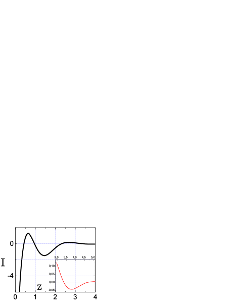
Figure 14: (Color online) Dimensionless function, ${\mathcal{I}}(z)$, describing the shape of a zero-bias anomaly in regime I, is plotted from Eq. (100) versus dimensionless energy, $z=\omega/\omega_{0}$. Inset in the lower-right corner: enlarged plot of ${\mathcal{I}}(z)$ in the domain $3<z<5$.

IX Zero-bias anomaly in averaged density of states in regime II

IX.1 Three polarization operators: Averaging of the net magnetic phase factor over realizations of random magnetic field

To derive analytical expressions for $\delta\nu^{(+)}(\omega)$ and $\delta\nu^{(-)}(\omega)$ one has to perform averaging of Eqs. (VII.2), (VII.2) over realizations of the random field. Such an averaging has already been carried out for the Friedel oscillations. In the latter case we had averaged $\langle\exp\left(2i\delta\varphi_{0\rightarrow{\bf r}}\right)\rangle$. In the case of the density of states, the exponents to be averaged are $\langle\exp\left(2i\delta\varphi_{\Sigma}^{(\pm)}\right)\rangle$, defined by Eqs. (74), (75). Our most important observation is that the net phase $\delta\varphi_{\Sigma}^{(-)}=\delta\varphi_{0\rightarrow{\bf r}_{1}}+\delta\varphi_{{\bf r}_{1}\rightarrow{\bf r}_{2}}+\delta\varphi_{{\bf r}_{2}\rightarrow 0}$ does not contain integrals of $\Lambda^{2}(x)$, since they cancel out. This can be clearly seen from Eq. (32). Instead, $\delta\varphi_{\Sigma}^{(-)}$ is expressed via integrals of $\Lambda(x)$ in the first power as follows

$$\delta\varphi_{\Sigma}^{(-)}=\frac{1}{\Phi_{0}^{2}k_{\text{\tiny{F}}}}\Biggl{[}\frac{1}{r_{1}}\left(\int_{0}^{r_{1}}dx\Lambda(x)\right)^{2}+\frac{1}{r_{2}-r_{1}}$$ (105)

$$\times\left(\int_{r_{1}}^{r_{2}}dx\Lambda(x)\right)^{2}-\frac{1}{r_{2}}\left(\int_{0}^{r_{2}}dx\Lambda(x)\right)^{2}\Biggr{]}.$$

This cancellation, as we demonstrate below, has a dramatic consequence for the average $\langle\exp(i\delta\varphi_{\Sigma})\rangle$. It turns out that, while $\langle\exp(i\delta\varphi_{0\rightarrow{\bf r}})\rangle$ decays with $r$ exponentially, the average $\langle\exp(i\delta\varphi_{\Sigma})\rangle$ falls off only as a power law. This, in turn, leads to a slow decay of a zero-bias anomaly, $\delta\nu(\omega/\omega_{1})$, with $\omega$.

On the technical level, cancellation of $\int dx\Lambda^{2}(x)$ terms leads to a drastic simplification of the disorder averaging of Eqs. (VII.2), (VII.2) in the regime II, as compared to the averaging of the Friedel oscillations in Section V.2, since the averaging of $\exp(2i\delta\varphi_{\Sigma})$ can be performed with the help of the Hubbard-Stratonovich transformation. For the purpose of functional averaging, it is convenient to rewrite Eq. (105) in a slightly different form

$$\delta\varphi_{\Sigma}^{(-)}=\frac{1}{\Phi_{0}^{2}k_{\text{\tiny{F}}}(r_{2}-r_{1})}\Biggl{[}\sqrt{\frac{r_{2}}{r_{1}}}\int_{0}^{r_{1}}dx\Lambda(x)$$ (106)

$$-\sqrt{\frac{r_{1}}{r_{2}}}\int_{0}^{r_{2}}dx\Lambda(x)\Biggr{]}^{2}.$$

Subsequent integration by parts yields the further simplification of Eq. (106)

$$\delta\varphi_{\Sigma}^{(-)}=\frac{1}{\Phi_{0}^{2}k_{\text{\tiny{F}}}(r_{2}-r_{1})}\Biggl{[}\sqrt{\frac{r_{2}}{r_{1}}}\int_{0}^{r_{1}}dx\;(r_{1}-x)h(x,0)$$

$$-\sqrt{\frac{r_{1}}{r_{2}}}\int_{0}^{r_{2}}dx\;(r_{2}-x)h(x,0)\Biggr{]}^{2}.\qquad\qquad$$ (107)

Now the averaging over realizations of $h(x,y)$ can be performed by a sequence of standard steps outlined below.

IX.1.1 Averaging procedure

Using Eq. (105) we rewrite the definition of average $\bigl{\langle}\exp(2i\delta\varphi_{\Sigma})\bigr{\rangle}$ by introducing the auxiliary integration variable, $c$

$$\Bigl{\langle}\exp\{2i\delta\varphi_{\Sigma}^{(-)}\}\Bigr{\rangle}=\int_{-\infty}^{\infty}\!dc\;\exp\left(-ic^{2}\right)\Biggl{\langle}\delta\Biggl{(}c-\frac{\sqrt{2}}{\Phi_{0}k_{\text{\tiny{F}}}^{1/2}\sqrt{r_{2}-r_{1}}}\left[\sqrt{\frac{r_{2}}{r_{1}}}\int_{0}^{r_{1}}dx\;(r_{1}-x)h(x,0)\right.$$

$$\left.-\sqrt{\frac{r_{1}}{r_{2}}}\int_{0}^{r_{2}}dx\;(r_{2}-x)h(x,0)\right]\Biggr{)}\Biggr{\rangle}_{h(x,y)},$$ (108)

where the averaging $\langle\dots\rangle_{h(x,y)}$ is defined by Eq. (V.2.2). Next we use the following integral representation of the $\delta$-function in Eq. (IX.1.1)

$$\Bigl{\langle}\exp\{2i\delta\varphi_{\Sigma}^{(-)}\}\Bigr{\rangle}=\int_{-\infty}^{\infty}\!dc\;\exp\left(-ic^{2}\right)\int_{-\infty}^{\infty}\!\frac{dt}{2\pi}e^{ict}\Biggl{\langle}\exp\Biggl{\{}-it\sqrt{2}\left[\sqrt{\frac{r_{2}}{r_{1}}}\int_{0}^{r_{1}}\frac{dx\;(r_{1}-x)h(x,0)}{\Phi_{0}k_{\text{\tiny{F}}}\sqrt{r_{2}-r_{1}}}\right.$$

$$\left.-\sqrt{\frac{r_{1}}{r_{2}}}\int_{0}^{r_{2}}\frac{dx\;(r_{2}-x)h(x,0)}{\Phi_{0}k_{\text{\tiny{F}}}\sqrt{r_{2}-r_{1}}}\right]\Biggr{\}}\Biggr{\rangle}_{h(x,y)}.$$ (109)

Now the integration over $c$ can be performed explicitly, yielding

$$\Bigl{\langle}\exp\{2i\delta\varphi_{\Sigma}^{(-)}\}\Bigr{\rangle}=\sqrt{\frac{\pi}{2}}e^{-i\pi/4}\int_{-\infty}^{\infty}\!\frac{dt}{2\pi}e^{it^{2}/4}\Biggl{\langle}\exp\Biggl{\{}-it\sqrt{2}\left[\sqrt{\frac{r_{2}}{r_{1}}}\int_{0}^{r_{1}}\frac{dx\;(r_{1}-x)h(x,0)}{\Phi_{0}k_{\text{\tiny{F}}}\sqrt{r_{2}-r_{1}}}\right.$$

$$\left.-\sqrt{\frac{r_{1}}{r_{2}}}\int_{0}^{r_{2}}\frac{dx\;(r_{2}-x)h(x,0)}{\Phi_{0}k_{\text{\tiny{F}}}\sqrt{r_{2}-r_{1}}}\right]\Biggr{\}}\Biggr{\rangle}_{h(x,y)}.$$ (110)

It follows from Eq. (IX.1.1) that evaluation of $\Bigl{\langle}\exp\{2i\delta\varphi_{\Sigma}^{(-)}\}\Bigr{\rangle}$ reduces to the Gaussian averaging of the exponent of a linear in $h(x)$ functional, which is standard

$$\!\!\!\!\!\!\!\Bigg{\langle}\!\exp\left\{-it\int_{0}^{r_{2}}dx\int_{-\infty}^{\infty}dyh(x,y)f(x)\delta(y)\right\}\!\Bigg{\rangle}_{h(x,y)}\!\!\!\!\!\!=$$ (111)

$$\!\!\!\!\exp\left\{-\frac{t^{2}}{4}\int_{0}^{r_{2}}dx_{1}\int_{0}^{r_{2}}dx_{2}f(x_{1})K(x_{1},0,x_{2},0)f(x_{2})\right\},$$

where $K(x_{1},0,x_{2},0)$ is related to the correlator of the random field Eq. (1) as follows $K(x_{1},0,x_{2},0)=h_{0}^{2}\text{\large K}(|x_{1}-x_{2}|/\xi)$. Subsequent integration over $t$ yields the final result

$$\Bigl{\langle}\exp\{2i\delta\varphi_{\Sigma}^{(-)}\}\Bigr{\rangle}\qquad\qquad\qquad\qquad\qquad\qquad\qquad\;\;\;$$ (112)

$$=\frac{1}{\sqrt{1+i\int_{0}^{r_{2}}\int_{0}^{r_{2}}dx_{1}dx_{2}f(x_{1})\text{K}(x_{1},0,x_{2},0)f(x_{2})}}.$$

As seen from Eq. (IX.1.1) the function $f(x)$ in Eq. (111) has the form

$$f_{-}(x) = \frac{\sqrt{2}}{\Phi_{0}k_{\text{\tiny{F}}}^{1/2}\sqrt{r_{2}-r_{1}}}\Biggl{[}\sqrt{\frac{r_{2}}{r_{1}}}(r_{1}-x)\theta(r_{1}-x)$$ (113)

$$- \sqrt{\frac{r_{1}}{r_{2}}}(r_{2}-x)\Biggr{]}.$$

Averaging of $\exp\left\{i\delta\varphi_{\Sigma}^{(+)}\right\}$ is performed similarly, and also yields Eq. (111) with $f(x)$ having the form

$$f_{+}(x) = \frac{\sqrt{2}}{\Phi_{0}k_{\text{\tiny{F}}}^{1/2}\sqrt{r_{2}}}\Biggl{[}\sqrt{\frac{r_{1}+r_{2}}{r_{1}}}(r_{1}-x)\theta(r_{1}-x)$$ (114)

$$- \sqrt{\frac{r_{1}}{r_{1}+r_{2}}}(r_{1}+r_{2}-x)\Biggr{]}.$$

We emphasize that expression Eq. (112) is general, and is valid for arbitrary, $h_{0}$ and $\xi$, i.e., in both regimes I and II. For the regime I, we had already performed the averaging over realizations of the random field. With regard to Eq. (112), regime I corresponds to replacement of the correlator by unity. In regime II, the distances $r_{1},r_{2}$ are much larger than $\xi$. For this reason, in regime II, the correlator in Eq. (112) can be replaced by $\sqrt{2\pi}\gamma\xi\delta(x_{1}-x_{2})$, with $\gamma$ defined by Eq. (56). Then the averages $\langle\exp\{2i\delta\varphi_{\Sigma}^{(-)}\}\rangle$ and $\langle\exp\{2i\delta\varphi_{\Sigma}^{(+)}\}\rangle$ can be expressed in terms of dimensionless ratios

$$\varrho_{1}=\frac{r_{1}}{\sqrt{6}r_{\text{\tiny{II}}}},~{}~{}~{}~{}\varrho_{2}=\frac{r_{2}}{\sqrt{6}r_{\text{\tiny{II}}}},$$ (115)

where the characteristic length, $r_{\text{\tiny{II}}}$, is defined by Eq. (63).

Eq. (112) and analogous expression for $\langle\exp\{2i\delta\varphi_{\Sigma}^{(+)}\}\rangle$ are sufficient to perform the averaging over realizations of random magnetic field in Eqs. (VII.2), (VII.2). However, averaged Eqs. (VII.2), (VII.2) contain the real and imaginary parts

$$\langle\exp\{2i\delta\varphi_{\Sigma}^{(\pm)}\}\rangle={\mathcal{U}}_{1}^{\pm}(\varrho_{1},\varrho_{2})+i~{}{\mathcal{U}}_{2}^{\pm}(\varrho_{1},\varrho_{2})$$ (116)

of the average exponents, separately. The expressions for ${\mathcal{U}}_{1}^{\pm}$ and ${\mathcal{U}}_{2}^{\pm}$ readily follow after replacing correlator by delta-function and performing integrations over $x_{1}$ and $x_{2}$ in Eq. (112)

$${\mathcal{U}}_{1}^{-}\!=\!\frac{\sqrt{\sqrt{\varrho_{1}^{2}(\varrho_{2}\!-\!\varrho_{1})^{2}\!+\!1}\!+\!1}\!+\!\sqrt{\sqrt{\varrho_{1}^{2}(\varrho_{2}\!-\!\varrho_{1})^{2}\!+\!1}\!-\!1}}{\sqrt{2}\sqrt{\varrho_{1}^{2}(\varrho_{2}-\varrho_{1})^{2}+1}}\!,$$

$${\mathcal{U}}_{2}^{-}\!=\!\frac{\sqrt{\sqrt{\varrho_{1}^{2}(\varrho_{2}\!-\!\varrho_{1})^{2}\!+\!1}\!+\!1}\!-\!\sqrt{\sqrt{\varrho_{1}^{2}(\varrho_{2}\!-\!\varrho_{1})^{2}\!+\!1}\!-\!1}}{\sqrt{2}\sqrt{\varrho_{1}^{2}(\varrho_{2}-\varrho_{1})^{2}+1}}\!,$$

$${\mathcal{U}}_{1}^{+}=\frac{\sqrt{\sqrt{\varrho_{1}^{2}\varrho_{2}^{2}+1}+1}+\sqrt{\sqrt{\varrho_{1}^{2}\varrho_{2}^{2}+1}-1}}{\sqrt{2}\sqrt{\varrho_{1}^{2}\varrho_{2}^{2}+1}}\!,$$

$${\mathcal{U}}_{2}^{+}=\frac{\sqrt{\sqrt{\varrho_{1}^{2}\varrho_{2}^{2}+1}+1}-\sqrt{\sqrt{\varrho_{1}^{2}\varrho_{2}^{2}+1}-1}}{\sqrt{2}\sqrt{\varrho_{1}^{2}\varrho_{2}^{2}+1}}.$$

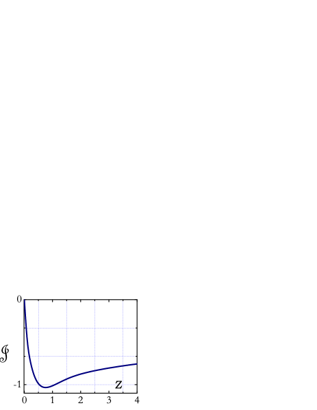
Figure 15: (Color online) Dimensionless density of states in regime II, ${\mathcal{J}}(z)={\mathcal{J}}^{+}(z)+{\mathcal{J}}^{-}(z)$, is plotted in the units of $(\nu_{0}{\mathcal{D}})$ from Eqs. (IX.1.1), (IX.1.1), (IX.1.1), (IX.1.1) versus dimensionless frequency, $z=\omega/\omega_{1}$, where $\omega_{1}$ is defined by Eq. (127) and ${\mathcal{D}}$ is defined by Eq. (122) .

Final expressions for the contributions $\langle\delta\nu^{-}(\omega)\rangle$ and $\langle\delta\nu^{+}(\omega)\rangle$ to the averaged density of states in the second regime are obtained by performing integration over $\Omega$ in Eqs. (VII.2) and (VII.2) and using Eqs. (IX.1.1)-(IX.1.1). We present this expression in the form similar to Eq. (97)

$$\Bigl{\langle}\frac{\delta\nu^{\pm}(\omega)}{\nu_{0}}\Bigr{\rangle}={\mathcal{D}}~{}{\mathcal{J}}^{\pm}\left(\frac{\omega}{\omega_{1}}\right),$$ (121)

where the prefactor ${\mathcal{D}}$ is defined as

$${\mathcal{D}}=-\frac{(\nu_{0}V)^{3}}{6^{3/4}(\pi k_{\text{\tiny{F}}}r_{\text{\tiny{II}}})^{3/2}},$$ (122)

and the dimensionless functions ${\mathcal{J}}^{\pm}$ are the following integrals over $\varrho_{1}$, $\varrho_{2}$

$${\mathcal{J}}_{1}^{-}(z)=\frac{1}{4}\int_{\varrho_{2}>\varrho_{1}}\frac{d\varrho_{1}d\varrho_{2}}{(\varrho_{1}\varrho_{2})^{3/2}}(\varrho_{2}-\varrho_{1})^{1/2}\Bigl{(}{\mathcal{U}}_{1}^{-}(\varrho_{1},\varrho_{2})-1\Bigr{)}\Biggl{(}\frac{\rho_{1}+\rho_{2}}{\rho_{1}\rho_{2}}\sin\left[\frac{\pi}{4}+2z(\varrho_{2}-\varrho_{1})\right]$$

$$-\frac{1}{\rho_{1}}\sin\left[\frac{\pi}{4}+2z\varrho_{2}\right]-\frac{1}{\rho_{2}}\sin\left[\frac{\pi}{4}-2z\varrho_{1}\right]\Biggr{)},$$ (123)

$${\mathcal{J}}_{2}^{-}(z)=\frac{1}{4}\int_{\varrho_{2}>\varrho_{1}}\frac{d\varrho_{1}d\varrho_{2}}{(\varrho_{1}\varrho_{2})^{3/2}}(\varrho_{2}-\varrho_{1})^{1/2}\Bigl{(}{\mathcal{U}}_{2}^{-}(\varrho_{1},\varrho_{2})-1\Bigr{)}\Biggl{(}\frac{\rho_{1}+\rho_{2}}{\rho_{1}\rho_{2}}\cos\left[\frac{\pi}{4}+2z(\varrho_{2}-\varrho_{1})\right]$$

$$-\frac{1}{\rho_{1}}\cos\left[\frac{\pi}{4}+2z\varrho_{2}\right]-\frac{1}{\rho_{2}}\cos\left[\frac{\pi}{4}-2z\varrho_{1}\right]\Biggr{)},$$ (124)

$${\mathcal{J}}_{1}^{+}(z)=\frac{1}{4}\int_{\varrho_{2}>\varrho_{1}}\frac{d\varrho_{1}d\varrho_{2}}{(\varrho_{1}\varrho_{2})^{3/2}(\varrho_{1}+\varrho_{2})^{1/2}}\biggl{\{}\Bigl{(}{\mathcal{U}}_{1}^{+}(\varrho_{1},\varrho_{2})-1\Bigr{)}\Bigl{(}\cos\left[\frac{\pi}{4}+2z(\varrho_{1}+\varrho_{2})\right]-\frac{1}{\sqrt{2}}\Bigr{)}$$

$$+\Bigl{(}{\mathcal{U}}_{2}^{+}(\varrho_{1},\varrho_{2})-1\Bigr{)}\Bigl{(}\sin\left[\frac{\pi}{4}+2z(\varrho_{1}+\varrho_{2})\right]-\frac{1}{\sqrt{2}}\Bigr{)}\biggl{\}},$$ (125)

$${\mathcal{J}}_{2}^{+}(z)=\frac{z}{2}\int_{\varrho_{2}>\varrho_{1}}\frac{d\varrho_{1}d\varrho_{2}}{(\varrho_{1}\varrho_{2})^{3/2}}(\varrho_{1}+\varrho_{2})^{1/2}\biggl{\{}\Bigl{(}{\mathcal{U}}_{1}^{+}(\varrho_{1},\varrho_{2})-1\Bigr{)}\sin\left[\frac{\pi}{4}+2z(\varrho_{1}+\varrho_{2})\right]$$

$$-\Bigl{(}{\mathcal{U}}_{2}^{+}(\varrho_{1},\varrho_{2})-1\Bigr{)}\sin\left[\frac{\pi}{4}-2z(\varrho_{1}+\varrho_{2})\right]\biggl{\}},$$ (126)

where $z=\omega/\omega_{1}$ is the dimensionless frequency. The new energy scale is related to the characteristic length, $r_{\text{\tiny{II}}}$, in the second regime in a usual way

$$\omega_{1}=\frac{v_{\text{\tiny{F}}}}{\sqrt{6}r_{\text{\tiny{II}}}}.$$ (127)

The second regime corresponds to long distances, $r_{\text{\tiny{II}}}>\xi$, travelled by electron. This is reflected in the fact that the frequency $\omega_{1}$ is smaller than $\omega_{0}$-the characteristic frequency for the first regime. Using Eq. (63), we can establish the relation between $\omega_{0}$ and $\omega_{1}$, namely, $\omega_{1}\sim\omega_{0}\varepsilon^{1/6}$, where $\varepsilon$ is the small parameter, defined by Eq. (12). We emphasize that the second regime exists only if the condition $\varepsilon\ll 1$ is met.

It is important to compare the scale $\omega_{1}$ to the “diffusive” energy scale $\omega_{\text{\tiny diff}}\sim v_{\text{\tiny F}}/l_{\text{\tiny tr}}$, where $l_{\text{\tiny tr}}$ is the transport mean free path. In the regime II we haveMirlin1

$$l_{\text{\tiny tr}}\sim v_{\text{\tiny F}}\left(k_{\text{\tiny F}}\xi\right)^{2}\left[\frac{v_{\text{\tiny F}}h_{0}^{2}\xi^{3}}{\Phi_{0}^{2}}\right]^{-1}=\frac{k_{\text{\tiny F}}^{2}\Phi_{0}^{2}}{h_{0}^{2}\xi}.$$ (128)

In this estimate the combination, $h_{0}^{2}\xi^{3}v_{\text{\tiny F}}/\Phi_{0}^{2}$, stands for a single-particle scattering rate, calculated from the golden rule, with $h_{0}^{2}\xi^{2}/\Phi_{0}^{2}$ coming from the square of the matrix element; the factor $\left(k_{\text{\tiny F}}\xi\right)^{2}$ accounts for the small-angle scattering. Eq. (128) leads to the following relation between the transport mean free path and $r_{\text{\tiny II}}$

$$\Bigl{(}\frac{l_{\text{\tiny tr}}}{k_{\text{\tiny F}}}\Bigr{)}^{1/2}\sim r_{\text{\tiny II}}\sim\frac{\xi}{\sqrt{\varepsilon}}.$$ (129)

As follows from Eq. (129), the distance $r_{\text{\tiny II}}$, over which the phase of the Friedel oscillations is preserved, is intermediate between $l_{\text{\tiny tr}}$ and $\xi$. Indeed, the ratio $l_{\text{\tiny tr}}/r_{\text{\tiny II}}$ is $\sim k_{\text{\tiny F}}r_{\text{\tiny II}}\sim k_{\text{\tiny F}}\xi/\sqrt{\varepsilon}$. This ratio is large both because $k_{\text{\tiny F}}\xi\gg 1$ and because $\varepsilon\ll 1$. Thus we conclude that the energy scale, $\omega_{1}$, is much larger than $\omega_{\text{\tiny diff}}$, since $\omega_{\text{\tiny diff}}/\omega_{1}$ is $\sim r_{\text{\tiny II}}/l_{\text{\tiny tr}}\ll 1$, i.e., the conventional diffusive zero-bias anomaly develops at frequencies much smaller than the width of the zero-bias anomaly in regime II.

IX.2 Discussion

Dimensionless density of states, ${\mathcal{J}}={\mathcal{J}}^{-}+{\mathcal{J}}^{+}$, is plotted in Fig. 15. It is seen that the function ${\mathcal{J}}(z)$ exhibits pronounced minimum at $z\approx 0.75$, which is followed by a monotonous decay. This behavior should be contrasted to the dimensionless density of states in the regime I, plotted in Fig. 14. The difference is that the function $\mathcal{I}$ exhibits damped oscillations with alternating maxima and minima, while ${\mathcal{J}}$ contains only a single minimum. This difference is not unexpected on qualitative grounds. Indeed, the distance $\sim r_{\text{\tiny I}}$, at which the oscillations are formed in regime I, is much smaller than the correlation radius, $\xi$, while the characteristic distance, $\sim r_{\text{\tiny II}}$, in regime II is much bigger than $\xi$. Therefore, it is remarkable that ${\mathcal{J}}(z)$ exhibits even a single minimum. However, qualitative difference between ${\mathcal{I}(z)}$ and ${\mathcal{J}}(z)$ at large $z$ is much harder to trace from their respective representations as double integrals over $\rho_{1}$ and $\rho_{2}$ [see Eqs. (100), (IX.1.1), (IX.1.1), (IX.1.1), (IX.1.1)]. The structure of one of several contributions to ${\mathcal{I}}(z)$ and ${\mathcal{J}}(z)$ can be loosely rewritten as

I $$: \!\!\!\quad\int_{0}^{\infty}\int_{0}^{\infty}\frac{d\rho_{1}d\rho_{2}}{(\rho_{1}\rho_{2})^{3/2}}\sqrt{\rho_{1}+\rho_{2}}\;\frac{\sin z\left(\rho_{1}+\rho_{2}\right)}{\sqrt{1+\rho_{1}^{2}\rho_{2}^{2}(\rho_{1}+\rho_{2})^{2}}},$$

II $$: \!\!\!\quad\int_{0}^{\infty}\int_{0}^{\infty}\frac{d\rho_{1}d\rho_{2}}{(\rho_{1}\rho_{2})^{3/2}}\sqrt{\rho_{1}+\rho_{2}}\;\frac{\sin z\left(\rho_{1}+\rho_{2}\right)}{\sqrt{1+\rho_{1}^{2}\rho_{2}^{2}}}.$$

The integrands in Eq. (IX.2) and Eq. (IX.2) differ only by the structure of the denominators. This difference can be traced to Eq. (112) in which the correlator is set either constant (regime I) or a $\delta$-function (regime II). From the form of the contribution Eq. (IX.2), it is not obvious at all that the large-$z$ behavior is determined by well-defined values $\rho_{1}=\rho_{2}=\rho_{0}$ in the complex plane, with $\rho_{0}$ satisfying $1+\rho_{0}^{6}=0$, so that the contribution is oscillatory Eq. (VIII). This fact was established above by taking the large-$z$ asymptote prior to the averaging over realizations. It is also supported by numerics in Fig. 14.

Monotonous behavior of ${\mathcal{J}}(z)$ at large $z$ implies that the integral Eq. (IX.2) is not dominated by distinct complex $\rho_{1}=\rho_{2}=\tilde{\rho}_{0}$, such that $1+\tilde{\rho}_{0}^{4}=0$. The only vague explanation of this is that denominator, $\sqrt{1+\rho_{1}^{2}\rho_{2}^{2}(\rho_{1}+\rho_{2})^{2}}$, in Eq. (IX.2) fixes $\rho_{1}\approx\rho_{2}\approx\rho_{0}$ much more efficiently that the denominator, $\sqrt{1+\rho_{1}^{2}\rho_{2}^{2}}$, in Eq. (IX.2) fixes $\rho_{1}$, $\rho_{2}$ near $\tilde{\rho}_{0}$.

X Implications

X.1 Half-filled Landau level

Experimental situation of a two-dimensional electron gas placed in inhomogeneous magnetic field can be created artificially, see, e.g., Refs. Geim90, ; bending90, ; Geim92, ; Geim94, ; smith94, ; mancoff95, ; gusev96, ; gusev00, ; rushforth04, . This situation also emerges in electron gas in a strong constant magnetic field, when the filling factor of the lowest Landau level is close to $1/2$. In the latter case, constant field transforms electrons into composite fermions Jain ; HLR , with well defined Fermi surface composite0 ; composite1 ; composite2 ; composite3 ; composite4 , while the randomness of magnetic field is due to spatial inhomogeneity of the electron density. Transport properties of noninteracting gas of composite fermions under these conditions were considered theoretically in Refs. chklovskii94, ; chklovskii95, ; Falko94, ; Khveshchenko96, ; Simons99, ; Shelankov00, ; Mirlin1, ; Mirlin2, ; Mirlin3, .

With regard to the tunnel density of states near the half-filling, for the case of homogeneous gas, it was addressed theoretically in Refs. He93, ; Shytov98, ; Shytov01, both for tunneling into the bulk and into the edge. Unlike interacting homogeneous electron gas,mishchenko02 composite fermions are expected to exhibit a zero-bias anomaly even without inhomogeneityHe93 ; Shytov98 ; Shytov01 . This difference between composite fermions and free electrons can be traced to the form of density-density correlator of composite fermions at small momentaHLR . Namely, the pole of this correlator defines the mode of neutral excitations with dispersion $\omega\propto iq^{3}$, even slower than the diffusive mode in the presence of disorder. Resulting suppression of tunneling into the edge of homogeneous electron gas at half filling, predicted in Refs. Shytov98, , Shytov01, , turned out to be stronger than in the experimentChang1 ; Chang2 .

It is convenient to express random static magnetic field originating from spatial inhomogeneity with magnitude $\delta n$, in the units of the cyclotron frequency

$$\frac{\delta\omega_{c}}{\Omega_{1/2}}=\frac{2\delta n}{n_{1/2}},$$ (132)

where $n_{1/2}$ is concentration of electrons at which the filling factor in the field, $\Omega_{1/2}$, is equal to $1/2$. Density fluctuations not only smear out the “intrinsic” zero-bias anomaly, but also give rise to the smooth-disorder-induced zero-bias anomaly, studied in the present paper. Quantitatively, we predict the following relation between the width of zero-bias anomaly and the magnitude, $\delta n$ of the density fluctuations

$$\omega_{0}\sim\Omega_{1/2}\Biggl{(}\frac{\delta n}{n_{1/2}}\Biggr{)}^{2/3}.$$ (133)

This relation follows directly from Eq. (13) and applies for smooth fluctuations with spatial scale, $\xi$, satisfying the condition

$$n_{1/2}\xi^{2}>\Biggl{(}\frac{n_{1/2}}{\delta n}\Biggr{)}^{4/3}.$$ (134)

This condition is equivalent to the condition $\varepsilon>1$, where the parameter $\varepsilon$ is defined by Eq. (12). In the opposite case of “fast” fluctuations the width, $\omega_{1}$, is given by

$$\omega_{1}\sim\Omega_{1/2}\left[n_{1/2}\xi^{2}\right]^{1/4}\left(\frac{\delta n}{n_{1/2}}\right),$$ (135)

as follows from Eq. (13). Concerning the magnitude of the anomaly, Eqs. (99) and (122) predict $\delta\nu/\nu_{0}\sim\left(\delta n/n_{1/2}\right)$ for slow fluctuations Eq. (133), and $\delta\nu/\nu_{0}\sim\left(\delta n/n_{1/2}\right)^{3/2}\Bigl{[}n_{1/2}\xi^{2}\Bigr{]}^{3/8}$ for the fast fluctuations Eq. (135), respectively.

Qualitative difference between the “intrinsic” zero-bias anomalyHe93 ; Shytov98 ; Shytov01 and inhomogeneity-induced zero-bias anomaly, considered in the present paper, is that the latter necessarily involves electron-electron scattering processes with momentum transfer $\approx 2k_{\text{\tiny F}}$. As was mentioned above, the intrinsic anomaly gets stronger towards the edgeShytov98 ; Shytov01 . We would like to emphasize that the anomaly due to the $2k_{\text{\tiny F}}$-processes also gets stronger towards the edge. The reason is that the average electron concentration decreases monotonically upon approaching the edge. This decrease translates into a non-fluctuating magnetic field, acting on composite fermionschklovskii95 , which increases towards the edge. Correction, $\delta\nu(\omega)$, to the density of states in this case is given by Eq. (81), and is plotted in Fig. 10. Then we conclude that the ratio of magnitudes, $\delta\nu_{\text{\tiny bulk}}/\delta\nu_{\text{\tiny edge}}$, is simply $\sim\left(\delta n_{\text{\tiny bulk}}/\delta n_{\text{\tiny edge}}\right)\ll 1$, where $\delta n_{\text{\tiny bulk}}$ and $\delta n_{\text{\tiny edge}}$ are the deviations of electron density from $n_{1/2}$ in the bulk and at the edge, respectively. The widths of $\delta\nu_{\text{\tiny bulk}}(\omega)$ and $\delta\nu_{\text{\tiny edge}}(\omega)$ are related as $\sim\left(\delta n_{\text{\tiny edge}}/\delta n_{\text{\tiny bulk}}\right)^{2/3}\ll 1$.

X.2 Spin-fermion model

Similarly to composite fermions, the dispersion of neutral excitations right at the critical point in the spin-fermion model is dominated by a slow mode,hertz76 ; millis93 $\omega\propto iq^{3}$. Outside the critical region, the propagator of the neutral excitations (bosons) in the spin-disordered phase has a conventional Ornstein-Zernike form $\chi(q)\propto 1/\left(q^{2}+\xi^{-2}\right)$, where $\xi$ is the correlation radius, which diverges at the critical point. Interaction of electrons with slow critical fluctuations can be viewed as scattering by the smooth disorder. The question that we will discuss below is how the growth of $\xi$, upon approaching the critical point, manifests itself in the behavior of the averaged (over the fluctuations of the order parameter) density of states. Our calculations demonstrate that the dimensionless parameter $\varepsilon$, defined by Eq. (12), plays a crucial role.

Traditionally, in the studies of the response functions, like spin susceptibility, of two-dimensional electrons near the quantum critical point, see, e.g., Refs. hertz76, ; millis93, ; belitz02, ; Chubukov04, ; Chubukov06, ; vojta07, , electrons are treated as ballistic. More specifically, they interact only with critical fluctuations, but not with each other. Transport at the quantum critical point was also considered for non-interacting ballisticNarozhny06 or diffusivePaul07 electrons that are scattered by bosonic excitations.

In all theoretical treatments of the spin-fermion model, modification of the response of the electron gas due to interaction with bosons was governed by the processes with small momentum transfer. Our main point is that incorporating direct electron-electron interactions into the spin-fermion model gives rise to a novel feature in the response of the electron gas near the critical point in spin-disordered phase. The underlying reason is that, while critical bosonic fluctuations are “smooth”, so that their momenta are $\ll k_{\text{\tiny F}}$, electron-electron interactions allow $2k_{\text{\tiny F}}$-processes. Then the physics, discussed in the present paper, emerges in the following way:

(i) interaction with slow bosonic fluctuations, curves slightly the electron trajectories;

(ii) interaction between the electrons, moving along slightly curved trajectories, generates a small energy scale, which reflects the “degree” of curving;

(iii) the degree of curving grows with correlation radius, $\xi$, of the bosonic excitations.

As a result, the character of critical fluctuations is reflected in the density of states, $\delta\nu(\omega)$, in a very nontrivial fashion. Namely, they give rise to the lively low-frequency feature and even aperiodic oscillations in $\delta\nu(\omega)$, as was demonstrated above. This suggests that information about proximity to the critical point can be inferred from tunneling experiments.

To quantify the above scenario, we will assume for simplicity Aharonov92 that bosonic critical fluctuations of magnetization, ${\bf S}({\bf r})$, interact with electron spins not as $\bm{\sigma}\cdot{\bf S}$, where $\bm{\sigma}$ are the Pauli matrices, but via the position-dependent Zeeman energy, $E_{\text{\tiny Z}}({\bf r})$, with characteristic magnitude, $E_{0}$. Assuming that the fluctuations, ${\bf S}({\bf r})$, are static, we get for correlator of random Zeeman energy, $E_{\text{\tiny Z}}({\bf r})$, the standard expression

$$\left\langle E_{\text{\tiny Z}}({\bf r})E_{\text{\tiny Z}}({\bf r}^{\prime})\right\rangle = E_{0}^{2}\int\frac{d{\bf q}}{2\pi}\;\frac{e^{i{\bf q}({\bf r}-{\bf r}^{\prime})}}{q^{2}+\xi^{-2}}$$ (136)

$$= E_{0}^{2}\;\text{K}_{0}\left(|x_{1}-x_{2}|/\xi\right),$$

where $\text{K}_{0}$ is the Macdonald function.

As a next step, we notice that the force, $\nabla E_{\text{\tiny Z}}({\bf r})$, curves the electron trajectories in the same way as random magnetic field, $h(x,y)$. This allows us to use general expressions Eqs. (VII.2), (VII.2) for the interaction correction to the density of states. We can also employ the result Eq. (112) for the general averaging procedure, i.e., to treat critical fluctuations as a disorder. With the help of Eq. (136) the result Eq. (112) assumes the form

$$\Bigl{\langle}\exp\{2i\delta\varphi_{\Sigma}^{(-)}\}\Bigr{\rangle}=\Bigl{[}1+iE_{0}^{2}\int_{0}^{r_{2}}\!\int_{0}^{r_{2}}dx_{1}dx_{2}$$ (137)

$$\times f_{-}(x_{1})f_{-}(x_{2})\partial_{x_{1}}\partial_{x_{2}}\text{K}_{0}\left(\frac{|x_{1}-x_{2}|}{\xi}\right)\Bigr{]}^{-1/2},$$

where the function $f_{-}$ is defined by Eq. (113) for the case of random magnetic field. For the case of random Zeeman energy, the prefactor, $1/\Phi_{0}k_{\text{\tiny F}}^{1/2}$, should be replaced by $k_{\text{\tiny F}}^{1/2}/E_{\text{\tiny F}}$. Characteristic energy scales can be now inferred from Eq. (137) on the basis of the following reasoning. Characteristic distances $r_{1}$, $r_{2}$ in Eq. (137) are determined by the condition

$$\int_{0}^{r_{2}}\!\int_{0}^{r_{2}}dx_{1}dx_{2}\text{K}_{0}\left(\frac{|x_{1}-x_{2}|}{\xi}\right)\frac{\partial}{\partial x_{1}}f_{-}(x_{1})\frac{\partial}{\partial x_{2}}f_{-}(x_{2})$$

$$\sim\frac{1}{E_{0}^{2}},$$ (138)

where we performed integration by parts in Eq. (137). Then the characteristic width of a zero-bias anomaly is equal to $\omega\sim v_{\text{\tiny F}}/r_{1}\sim v_{\text{\tiny F}}/r_{2}$.

Recall now, that in the case of random magnetic field, double integral in the left-hand side of Eq. (X.2) did not contain derivatives and was $\propto r_{2}^{3}$ in the regime I, and $\propto r_{2}^{2}\xi$ in regime II, respectively. This is because the function, $f_{-}(x_{1})$, is $\sim r_{2}^{1/2}$ at $x_{1}\sim r_{2}$, see Eq. (113). Due to the fact that the effective “force” in the spin-fermion model is $\propto\nabla E_{\text{\tiny Z}}({\bf r})$, the left-hand side in Eq. (X.2) is $\sim k_{\text{\tiny F}}r_{2}/E_{\text{\tiny F}}^{2}$ for $\xi\gg r_{2}$. In this limit, Eq. (X.2) yields (with logarithmic in $\xi/r_{2}$ accuracy)

$$r_{2}\sim k_{\text{\tiny F}}^{-1}\left(\frac{E_{\text{\tiny F}}}{E_{0}}\right)^{2}=\xi_{c},~{}~{}\omega\sim\frac{E_{0}^{2}}{E_{\text{\tiny F}}}=E_{c}.$$ (139)

Note that $E_{c}$ is independent of $\xi$. We conclude that, upon approaching the critical point, as the correlation radius exceeds the value $\xi_{c}$, the zero-bias anomaly “freezes”. Its form is shown in Fig. 14, and its magnitude is $\sim\left(E_{0}/E_{\text{\tiny F}}\right)^{3}$. An alternative way to recover the scales Eq. (139) is to notice that parameter $\varepsilon$, which is defined by Eq. (12) in context of random magnetic field, in the situation with random Zeeman energy acquires the form $\varepsilon=(k_{\text{\tiny F}}\xi)\left(E_{0}/E_{\text{\tiny F}}\right)^{2}$. Then $\xi_{c}$ given by Eq. (139) corresponds to $\varepsilon=1$, i.e., to the boundary of the regime I.

For $\xi<\xi_{c}$ the integral in the left-hand side of Eq. (X.2) is proportional to $\xi$ and is independent of $r_{2}$. Then Eq. (X.2) does not have a solution. Therefore, characteristic $r_{1}$ and $r_{2}$ in the expression for the density of states are $\sim\xi$, and the width of the anomaly is simply $\sim v_{\text{\tiny F}}/\xi=E_{c}(\xi_{c}/\xi)$. Concerning the magnitude of the anomaly at $\xi<\xi_{c}$, it should be estimated with the account that the integral in right-hand side of Eq. (137) is smaller than $1$ for all $r_{2}$. Therefore, $\Bigl{\langle}\exp\{2i\delta\varphi_{\Sigma}^{(-)}\}\Bigr{\rangle}$ in Eq. (137) can be approximately replaced by $\bigl{\{}1-(i/2\xi_{c})\left[r_{2}\Theta(\xi-r_{2})+\xi\Theta(r_{2}-\xi)\right]\bigr{\}}$, where the second term is a small correction. However, only this correction causes a zero-bias anomaly. Substituting this correction into Eq. (VII.2), we find the estimate for the magnitude,

$$\frac{\delta\nu}{\nu_{0}}\sim\left(\frac{E_{0}}{E_{\text{\tiny F}}}\right)^{3}\left(\frac{\xi_{c}}{\xi}\right)^{1/2}\sim\left(\frac{E_{0}}{E_{\text{\tiny F}}}\right)^{2}\frac{1}{(k_{\text{\tiny F}}\xi)^{1/2}}.$$ (140)

We conclude that, as $\xi$ grows and approaches $\xi_{c}$, the magnitude of the anomaly falls off as $1/\sqrt{\xi}$, and the anomaly narrows as $1/\xi$.

The remaining issue to discuss is whether or not the assumption that fluctuating Zeeman energy, $E_{\text{\tiny Z}}({\bf r})$, is static applies at relevant frequency and spatial scales, $E_{c}$ and $\xi_{c}$. For this purpose, we recall the correlator of Zeeman energies in the momentum space does not have a simple Ornstein-Zernike form but is rather $\left\langle|E_{\text{\tiny Z}}({\bf q})|^{2}\right\rangle\propto 1/\left(q^{2}+\xi^{-2}+\varsigma\omega/q\right)$, where the dynamic term, $\varsigma\omega/q$, describes the damping of bosons due to creation of electron-hole pairs. The prefactor $\varsigma$ (the Landau damping coefficient) is thus quadratic in coupling of electrons to the spin density fluctuations, i.e., $\varsigma\propto E_{0}^{2}$. For characteristic frequencies the dynamic term, $\varsigma(\omega/q)\sim\varsigma E_{c}\xi_{c}\sim\varsigma v_{\text{\tiny F}}$. Therefore, it is negligible only if the condition, $\xi_{c}^{-2}=k_{\text{\tiny F}}^{2}\left(E_{0}/E_{\text{\tiny F}}\right)^{4}\gg\varsigma v_{\text{\tiny F}}$, holds. With $\varsigma$ being proportional to $E_{0}^{2}$, the above condition is met for large enough coupling, $E_{0}$. In the opposite case, when the dynamic part of correlator dominates at $\omega\sim E_{c}$ and $q\sim\xi_{c}^{-1}$, the zero-bias anomaly develops only away from the critical point when $\xi$ becomes smaller than $(\varsigma v_{\text{\tiny F}})^{-1/2}$. Upon further departure from the critical point, our prediction $\delta\nu/\nu_{0}\propto\xi^{-1/2}$ and $\omega\sim v_{\text{\tiny F}}/\xi$ should apply. Note finally, that, directly at the critical point, the slow mode $\omega\approx iq^{3}/\varsigma$ gives rise to the “intrinsic” zero-bias anomaly,Chubukov06 similar to the composite fermions.

Appendix A Polarization operator in the coordinate space

Here we derive Eqs. (17) and (IV.1) for polarization operator in coordinate space using the known expression Stern67 for $\Pi({\bf q},\omega)$ in the momentum space. Since we are interested in behavior of $\Pi({\bf r},\omega)$ at distances $|{\bf r}|\gg k_{\text{\tiny{F}}}^{-1}$, it is sufficient to perform the Fourier transform

$$\Pi({\bf r},\omega)=\frac{1}{2\pi}\int\!d{\bf q}\;e^{i{\bf qr}}\;\Pi({\bf q},\omega),$$ (141)

using the asymptotes of $\Pi({\bf q},\omega)$ at small $q\ll k_{\text{\tiny{F}}}$ and at $q$ close to $2k_{\text{\tiny{F}}}$. The small-$q$ asymptote of $\Pi({\bf q},\omega)$ has the form

$$\Pi_{0}({\bf q},\omega)=-\nu_{0}\left[1+\frac{i\omega\;\Theta(qv_{\text{\tiny{F}}}-\omega)}{\sqrt{q^{2}v_{\text{\tiny{F}}}^{2}-\omega^{2}}}\right.$$

$$\left.~{}~{}~{}~{}~{}~{}~{}~{}~{}~{}~{}~{}~{}~{}~{}~{}+\frac{\omega\;\Theta(\omega-qv_{\text{\tiny{F}}})}{\sqrt{\omega^{2}-q^{2}v_{\text{\tiny{F}}}^{2}}}\right],$$ (142)

where $\Theta(x)$ is the step-function. The easiest way to perform the integration Eq. (141) is to first Fourier transform Eq. (A) with respect to frequency

$$-\frac{\Theta(qv_{\text{\tiny{F}}}-\omega)}{\sqrt{q^{2}-\left(\omega/v_{\text{\tiny{F}}}\right)^{2}}}+\frac{i\Theta(\omega-qv_{\text{\tiny{F}}})}{\sqrt{\left(\omega/v_{\text{\tiny{F}}}\right)^{2}-q^{2}}}\qquad$$

$$\qquad=\int_{0}^{\infty}\!\!ds\;J_{0}(qs)\;\exp\left\{\frac{i\omega\;s}{v_{\text{\tiny{F}}}}\right\}.$$ (143)

Substituting Eq. (A) into Eq. (A) and using the orthogonality relation $\int_{0}^{\infty}dq\;qJ_{0}(qs)J_{0}(qr)=\delta(r-s)/r$, we readily obtain

$$\Pi_{0}({\bf r},\omega)=-\frac{i\nu_{0}\omega}{v_{\text{\tiny{F}}}r}\exp\left\{\frac{i\omega\;r}{v_{\text{\tiny{F}}}}\right\}.$$ (144)

In order to calculate $\Pi_{2k_{\text{\tiny{F}}}}({\bf r},\omega)$ we use the form of polarization operator in momentum space for $|q-2k_{\text{\tiny{F}}}|\ll k_{\text{\tiny{F}}}$ and $\omega\ll E_{\text{\tiny{F}}}$

$$\Pi_{2k_{\text{\tiny{F}}}}({\bf q},\omega)=\nu_{0}\Biggl{[}1-\frac{1}{\sqrt{4k_{\text{\tiny{F}}}}}\qquad\qquad\qquad\qquad\qquad$$ (145)

$$\times\left(\sqrt{q-2k_{\text{\tiny{F}}}+\omega/v_{\text{\tiny{F}}}}+\sqrt{q-2k_{\text{\tiny{F}}}-\omega/v_{\text{\tiny{F}}}}\right)\Biggr{]},$$

where the square roots should be understood as $\sqrt{x}\rightarrow\text{sign}(x)\sqrt{x}$. Then the integral over ${\bf q}$ in Eq. (141) assumes the form

$$\Pi_{2k_{\text{\tiny{F}}}}({\bf r},\omega)=-\nu_{0}\int_{0}^{\infty}dq\;qJ_{0}(qr)\Bigl{[}\sqrt{q-2k_{\text{\tiny{F}}}+\omega/v_{\text{\tiny{F}}}}\;\;\;\;\;\;\;\;$$

$$+\sqrt{q-2k_{\text{\tiny{F}}}-\omega/v_{\text{\tiny{F}}}}\Bigr{]}\approx\sqrt{\frac{4k_{\text{\tiny{F}}}}{\pi r}}\int_{0}^{\infty}dq\cos\left(qr-\frac{\pi}{4}\right)\quad\quad\;\;$$

$$\times\Bigl{[}\sqrt{q-2k_{\text{\tiny{F}}}+\omega/v_{\text{\tiny{F}}}}+\sqrt{q-2k_{\text{\tiny{F}}}-\omega/v_{\text{\tiny{F}}}}\Bigr{]}\qquad\;\;\;$$ (146)

where we used that fact that $k_{\text{\tiny{F}}}r\gg 1$ and replaced the Bessel function by its large-$q$ asymptotics. Integration over variable $q$ in Eq. (A) is performed with the use of the identity

$$\int_{a}^{\infty}dz\;\cos z\sqrt{z-a}={\frac{\sqrt{\pi}}{2}}\sin\left(a+\frac{\pi}{4}\right),$$ (147)

and yields the zero-temperature limit of Eq. (IV.1).

Appendix B Polarization operator in a constant magnetic field

We start from the general expression aleiner95 for the polarizability in arbitrary magnetic field

$${\large{\Pi}}\;(q)=-\frac{2m}{\pi}\sum_{n_{1}=0}^{\infty}\sum_{n_{2}=0}^{\infty}\frac{(-1)^{(n_{2}-n_{1})}\bigl{(}f_{n_{1}}-f_{n_{2}}\bigr{)}}{{n_{2}-n_{1}}}$$

$$\times\exp(-q^{2}l^{2}/2)\;{\text{\large L}}_{n_{1}}^{n_{2}-n_{1}}\left(\frac{q^{2}l^{2}}{2}\right){\text{\large L}}_{n_{2}}^{n_{1}-n_{2}}\left(\frac{q^{2}l^{2}}{2}\right),$$ (148)

where ${\text{\large L}}_{n_{1}}^{n_{2}-n_{1}}(x)$ and ${\text{\large L}}_{n_{2}}^{n_{1}-n_{2}}(x)$ are the Laguerre polynomials, and $f_{n}=\bigl{\{}\exp\bigl{[}(n-N_{\mbox{\tiny F}})\hbar\omega_{c}/T\bigr{]}+1\bigr{\}}^{-1}$ is the Fermi distribution. At small $q\ll k_{\mbox{\tiny F}}$ Eq. (B) yields aleiner95 $\Pi\;\!(q)=-(m/\pi)\bigl{[}1-J_{0}^{2}(qR_{\mbox{\tiny L}})\bigr{]}$, i.e., the characteristic scale is $q\sim R_{\mbox{\tiny L}}^{-1}$. For $(q-2k_{\mbox{\tiny F}})\ll k_{\mbox{\tiny F}}$ it is convenient to perform the summation over the Landau levels with the help of the following integral representation of the Laguerre polynomial

$${\text{\large L}}_{m}^{n}(x)=\frac{1}{2\pi}\int_{0}^{2\pi}\!\!\frac{d\theta}{\left(1-e^{i\theta}\right)^{n+1}}\exp\left\{\frac{xe^{i\theta}}{e^{i\theta}-1}-im\theta\right\}.$$

In the vicinity $q=2k_{\mbox{\tiny F}}$ Eq. (B) contains a small factor $\exp(-q^{2}l^{2}/2)$. This factor is compensated by the product of Laguerre polynomials, since each of them is $\propto\exp(x/2)$, which comes from the exponent in Eq. (B) taken at $\theta=\pi$. With contribution from the vicinity $\theta=\pi$ dominating the integral (B), we can expand the integrand around this point as $\exp\bigl{[}x/2+i\pi m+i\phi(\psi)\bigr{]}/2^{n+1}$, where $\psi=(\theta-\pi)$, and the phase, $\phi(\psi)$, is equal to

$${\large\phi}(\psi)=\left({x\over 4}-m-\frac{n+1}{2}\right)\psi+\frac{x\psi^{3}}{48}.$$ (150)

Now we make use of the fact that only relatively small number $\sim(k_{\mbox{\tiny F}}l)^{2/3}\ll N_{\mbox{\tiny F}}$ of Landau levels around $E_{\mbox{\tiny F}}$ contribute to the sum Eq. (B). This suggests that we can present $n_{1}$ and $n_{2}$ as $n_{1}=N_{\mbox{\tiny F}}+m_{1}$ and $n_{2}=N_{\mbox{\tiny F}}-m_{2}$, respectively, and extend the sum over $m_{1}$, $m_{2}$ from $-\infty$ to $+\infty$. After that the summation over Landau levels can be easily carried out with the help of the following identity

$$\sum\limits_{m_{1},m_{2}=-\infty}^{\infty}\frac{f_{N_{\mbox{\tiny F}}-m_{1}}-f_{N_{\mbox{\tiny F}}+m_{2}}}{m_{1}+m_{2}}\qquad\qquad$$

$$\times\cos\bigl{[}(m_{1}-m_{2})\alpha+\beta\bigr{]}=\frac{2\pi^{2}T\cos\beta}{\hbar\omega_{c}\sinh\bigl{(}2\pi|\alpha|T/\hbar\omega_{c})}.$$ (151)

As a next step, we substitute the representation Eq. (B) of Laguerre polynomials with integrand expanded according to Eq. (150), into Eq. (B). Upon this substitution, we perform the summation over Landau levels using the relation Eq. (B). Then the double integral, which emerges in Eq. (B) as a result of representing the two laguerre polynomials Eq. (B), assumes the form

$$\int_{-\infty}^{\infty}\int_{-\infty}^{\infty}\frac{d\psi_{1}d\psi_{2}}{|\psi_{1}+\psi_{2}|}\qquad\qquad\qquad\qquad\qquad$$

$$\times\cos\left[\left(\psi_{1}^{3}+\psi_{2}^{3}\right)\frac{N_{\mbox{\tiny F}}}{12}-\left(\psi_{1}+\psi_{2}\right)\frac{\delta qR_{\mbox{\tiny L}}}{2}\right],$$ (152)

where $\delta q=q-2k_{\text{\tiny{F}}}$. Note, that integration over the difference, $(\psi_{1}-\psi_{2})$, in Eq. (B) can be performed explicitly. It is convenient to present the final result not for $\Pi(q)$, but rather for the derivative, $\Pi^{\prime}(q,T)=\partial\Pi(q,T)/\partial q$. Knowledge of $\Pi^{\prime}(q,T)$ is sufficient for finding the large-distance behavior of the potential, created by the short-range impurity. Indeed, this potential can be expressed directly through $\Pi^{\prime}(2k_{\mbox{\tiny F}}+Q)$ as follows

$$V_{H}(r)=\frac{V(2k_{\mbox{\tiny F}})g}{2(\pi k_{\mbox{\tiny F}}r)^{3/2}}\int_{-\infty}^{\infty}\!\!dQ\sin\!\left[(2k_{\mbox{\tiny F}}+Q)r-\!{\pi\over 4}\right]\times$$

$$\Pi^{\prime}(2k_{\mbox{\tiny F}}+Q,T).\qquad$$ (153)

At zero temperature and in a zero magnetic field we have $\Pi^{\prime}(q,0)\propto\theta(\delta q)/\sqrt{\delta q}$. At finite magnetic field and finate temperature, taking derivative of Eq. (B) with respect to $\delta q$, we arrive to the result

$$\Pi^{\prime}(q,T)=-\frac{2^{1/3}mT}{(\pi k_{\mbox{\tiny F}}{p_{0}})^{1/2}\epsilon_{0}}\int_{0}^{\infty}\frac{dx\;x^{1/2}}{\sinh(2\pi xT/\epsilon_{0})}$$

$$\times\sin\left(2^{2/3}\frac{\delta q}{p_{0}}\;x+\frac{1}{3}x^{3}+\frac{\pi}{4}\right).$$ (154)

In the limit $T\rightarrow 0$, substitution of Eq. (B) into Eq. (B) and integration over $Q$ reproduces Eq. (3).

Interestingly, for $T=0$, the integral Eq. (B) can be evaluated analytically

$$\Pi^{\prime}(q)=-\frac{m}{(k_{\mbox{\tiny F}}{p_{0}})^{1/2}}\;{\text{\large\it Ai}}\left(\frac{\delta q}{p_{0}}\right)\;{\text{\large\it Bi}}\left(\frac{\delta q}{p_{0}}\right),$$ (155)

where $Ai(z)$ is the Airy function, and $Bi(z)$ is another solution of the Airy equation defined, e.g., in Ref. book, . It is seen that the singularity at $q=2k_{\mbox{\tiny F}}$ is smeared by the magnetic field in a rather peculiar way: for positive $\delta q\gg p_{0}$ the $(\delta q)^{-1/2}$ zero-field behavior [see Eq. (A)] is restored. However, for large negative $\delta q/p_{0}$, the derivative $\Pi^{\prime}(q)$ approaches zero with oscillations, namely, as $\cos\bigl{[}4(|\delta q|/p_{0})^{3/2}/3\bigr{]}/(|\delta q|)^{1/2}$. As the difference $2k_{\mbox{\tiny F}}-q$ increases and becomes comparable to $k_{\mbox{\tiny F}}$, these oscillations cross over to the “classical” oscillationsaleiner95 $\Pi^{\prime}(q)\propto J_{0}(qR_{\mbox{\tiny L}})J_{1}(qR_{\mbox{\tiny L}})\propto\cos(2qR_{\mbox{\tiny L}})$.

Appendix C Evaluation of the functional integral

Upon combining Eqs. (58) and (V.2.2) the quadratic form in the exponent in the numerator of the functional integral Eq. (V.2.2) assumes the form

$$2i\delta\varphi(r)-W\{h\}=\frac{2i\varepsilon r^{3}}{\xi^{3}}\Biggl{\{}\frac{1}{12}\left[\int dq\;{\mathcal{A}}_{0,q}\right]^{2}+\sum_{n>0}c_{n}\Big{|}\int dq\;{\mathcal{A}}_{n,q}\Big{|}^{2}+\int dq\;{\mathcal{A}}_{0,q}{\mathcal{G}}\{{\mathcal{A}}_{n}\}\Biggr{\}}$$ (156)

$$-\frac{2r}{\gamma\xi}\sum_{n>0}\int\!dq\;\frac{|{\mathcal{A}}_{n,q}|^{2}}{\tilde{\mathcal{K}}(q)}-\frac{r}{\gamma\xi}\int\!dq\;\frac{|{\mathcal{A}}_{0,q}|^{2}}{\tilde{\mathcal{K}}(q)},$$

with numerical coefficients $c_{n}=1/2\pi^{2}n^{2}$ and $b_{n}=-c_{n}+i/2\pi n$ defined by Eq. (61). In the above expression we had introduced a short-hand notation

$${\mathcal{G}}\{{\mathcal{A}}_{n,q}\}=\sum_{n>0}\Bigl{[}b_{n}\int dq\;{\mathcal{A}}_{n,q}+b_{n}^{\ast}\int dq\;{\mathcal{A}}_{n,q}^{\ast}\Bigr{]}.$$ (157)

We adopt the following sequence of integration over the variables ${\mathcal{A}}_{n,q}$. First we integrate over ${\mathcal{A}}_{0,q}$ using the following decoupling

$${\text{\large H}}\{{\mathcal{G}}\}=\int\prod_{q}d{\mathcal{A}}_{0,q}\exp\Biggl{\{}-\frac{r}{\gamma\xi}\int\!dq\;\frac{|{\mathcal{A}}_{0,q}|^{2}}{\tilde{\mathcal{K}}(q)}+\frac{i\varepsilon r^{3}}{6\xi^{3}}\left[\int dq\;{\mathcal{A}}_{0,q}\right]^{2}+i{\mathcal{G}}\int dq\;{\mathcal{A}}_{0,q}\Biggr{\}}=$$ (158)

$$e^{-i\pi/4}\sqrt{\frac{3r^{3}}{2\pi\varepsilon\xi^{3}}}\int\prod_{q}d{\mathcal{A}}_{0,q}d{\mathcal{B}}_{0}\exp\Biggl{\{}-\frac{3ir^{3}{\mathcal{B}}_{0}^{2}}{2\varepsilon\xi^{3}}+i{\mathcal{B}}_{0}\int dq\;{\mathcal{A}}_{0,q}-\frac{r}{\gamma\xi}\int\!dq\;\frac{|{\mathcal{A}}_{0,q}|^{2}}{\tilde{\mathcal{K}}(q)}+i{\mathcal{G}}\int dq\;{\mathcal{A}}_{0,q}\Biggr{\}},$$

where we had introduced an auxiliary variable ${\mathcal{B}}_{0}$. Function ${\text{\large H}}\{{\mathcal{G}}\}$ combines all integrals in Eq. (156) containing ${\mathcal{A}}_{0,q}$. Subsequent integration first over the variables ${\mathcal{A}}_{0,q}$ and then over the auxiliary variable ${\mathcal{B}}_{0}$ yields

$${\text{\large H}}\{{\mathcal{G}}\}=\sqrt{\frac{\pi\xi\gamma}{ir\int dq\;\tilde{\mathcal{K}}(q)}}\frac{\exp\bigl{\{}i{\mathcal{F}}(r){\mathcal{G}}^{2}\bigr{\}}}{\sqrt{1-\frac{2i}{3}\left(\frac{r}{r_{\text{\tiny{II}}}}\right)^{2}}},$$

where we had used the definition $r_{\text{\tiny{II}}}=2\xi/\left(\sqrt{2\pi}\gamma\varepsilon\right)^{1/2}$. In Eq. (C) the complex function ${\mathcal{F}}(r)$ is defined as

$${\mathcal{F}}(r)=-\frac{3\varepsilon^{1/2}\left(\gamma\int\!dq\;\tilde{\mathcal{K}}(q)\right)^{3/2}}{16\left(\frac{r}{r_{\text{\tiny{II}}}}\right)^{3}+24i\left(\frac{r}{r_{\text{\tiny{II}}}}\right)}.$$

As a result of integration over ${\mathcal{A}}_{0,q}$ the exponent in the functional integral Eq. (156) assumes the form

$$i\sum_{n>0}{\tilde{c}}_{n}\Big{|}\int\!dq\;{\mathcal{A}}_{n,q}\Big{|}^{2}\qquad\qquad\qquad$$ (160)

$$\qquad\qquad\qquad-\frac{2r}{\gamma\xi}\sum_{n>0}\int\!dq\;\frac{|{\mathcal{A}}_{n,q}|^{2}}{\tilde{\mathcal{K}}(q)}+i{\mathcal{F}}(r){\mathcal{G}}^{2},$$

where ${\tilde{c}}_{n}$ is related to $c_{n}$ via a dimensionless factor

$${\tilde{c}}_{n}=\frac{2\varepsilon r^{3}}{\xi^{3}}c_{n}.$$ (161)

The first and the third terms in Eq. (160) contain squares of the linear combinations of ${\mathcal{A}}_{n,q}$. To decouple these squares, we introduce a set of auxiliary variables, $\alpha_{n},\alpha_{n}^{\ast}$ for the first term, and one auxiliary variable, $\alpha_{0}$ for the third term as follows

$$e^{i{\mathcal{V}}\left|\int\!dq\;{\mathcal{A}}_{n,q}\right|^{2}}=\frac{1}{2\pi}\int\!d\alpha_{n}d\alpha_{n}^{\ast}\exp\Bigl{\{}-i|\alpha_{n}|^{2}+{\mathcal{V}}^{1/2}\alpha_{n}^{\ast}\int\!dq\;{\mathcal{A}}_{n,q}-{\mathcal{V}}^{1/2}\alpha_{n}\int\!dq\;{\mathcal{A}}_{n,q}^{\ast}\Bigr{\}},$$ (162)

$$e^{i{\mathcal{F}}(r){\mathcal{G}}^{2}}=\frac{1}{\sqrt{4\pi{\mathcal{F}}(r)}}\int_{-\infty}^{\infty}d\alpha_{0}\exp\left\{-\frac{i\alpha_{0}^{2}}{4{\mathcal{F}}(r)}+i\alpha_{0}{\mathcal{G}}\right\}.$$

Note that $\text{Im}\left[1/{\mathcal{F}}(r)\right]<0$, so that the decoupling Eq. (C) of the quadratic in ${\mathcal{G}}$ term in the exponent of Eq. (C) is justified.

As a next step, we perform gaussian integration over the infinite set of variables, $\{{\mathcal{A}}_{n,q}\}$

$$\int d{\mathcal{A}}_{n,q}d{\mathcal{A}}_{n,q}^{\ast}\exp\Biggl{\{}\int\!dq\Bigl{[}-\frac{2r|{\mathcal{A}}_{n,q}|^{2}}{\gamma\xi{\tilde{\mathcal{K}}(q)}}+{\mathcal{A}}_{n,q}\left({\tilde{c}}_{n}^{1/2}\alpha_{n}^{\ast}+i\alpha_{0}b_{n}\right)\!+\!{\mathcal{A}}_{n,q}^{\ast}\left(-{\tilde{c}}_{n}^{1/2}\alpha_{n}+i\alpha_{0}b_{n}^{\ast}\right)\Bigr{]}\!\Biggr{\}}$$

$$\qquad=\frac{2i\pi}{(2r/\gamma\xi)\int\!dq\;\left[{\tilde{\mathcal{K}}(q)}\right]^{-1}}\exp\Bigl{\{}-\left|-i{\tilde{c}}_{n}^{1/2}\alpha_{n}^{\ast}+\alpha_{0}b_{n}\right|^{2}\frac{\gamma\xi}{2r}\int\!dq\;{\tilde{\mathcal{K}}(q)}\Bigr{\}}.$$ (164)

As follows from Eqs. (162) and (C), the integrals over all $\alpha_{n}$ are gaussian and can be easily evaluated

$$\int\frac{d\alpha_{n}d\alpha_{n}^{\ast}}{2\pi}\exp\Bigl{\{}-i|\alpha_{n}|^{2}-\left|-i{\tilde{c}}_{n}^{1/2}\alpha_{n}^{\ast}+\alpha_{0}b_{n}\right|^{2}\frac{\gamma\xi}{2r}\int\!dq\;{\tilde{\mathcal{K}}(q)}\Bigr{\}}$$

$$=\frac{2r}{2r-i\gamma\xi{\tilde{c}}_{n}\int\!dq{\tilde{\mathcal{K}}(q)}}\exp\Biggl{\{}\!-\frac{\gamma\xi\alpha_{0}|b_{n}|^{2}}{2r}\!\int\!dq{\tilde{\mathcal{K}}(q)}\!-\!\frac{{\tilde{c}}_{n}\left[\alpha_{0}|b_{n}|\gamma\xi\int\!dq{\tilde{\mathcal{K}}(q)}\right]^{2}}{4ir^{2}+2r\gamma\xi{\tilde{c}}_{n}\int\!dq{\tilde{\mathcal{K}}(q)}}\!\Biggr{\}}.$$ (165)

The remaining integral over $\alpha_{0}$ is also gaussian. Note now, that the denominator in Eq. (V.2.2), responsible for the normalization, can be evaluated by performing the same steps as above. This evaluation amounts to setting ${\tilde{c}}_{n}=0$ in Eq. (C) and taking the limit $r_{\text{\tiny{II}}}\rightarrow\infty$ in Eq. (C). As a result, the functional integral reduces to the ratio of the ordinary integrals

$$\langle e^{2i\delta\varphi(r)}\rangle=\frac{1}{\sqrt{1-\frac{2i}{3}\left(\frac{r}{r_{\text{\tiny{II}}}}\right)^{2}}}\left[\prod_{n=1}^{\infty}\frac{n^{2}}{n^{2}-2i(r/r_{\text{\tiny{II}}})^{2}/\pi^{2}}\right]\;\frac{\int_{-\infty}^{\infty}\!\!d\alpha_{0}\exp\left\{-w\alpha_{0}-u_{1}\alpha_{0}^{2}\right\}}{\int_{-\infty}^{\infty}\!\!d\alpha_{0}\exp\left\{-w\alpha_{0}-u_{0}\alpha_{0}^{2}\right\}},$$ (166)

where the coefficients $w$, and $u_{0}$ are defined as

$$w=\frac{\gamma\xi}{2r}\left[\sum_{n>0}|b_{n}|^{2}\right]\!\int\!dq{\tilde{\mathcal{K}}(q)},$$

$$u_{0}=\frac{r}{\xi}\Bigl{(}\int\!dq{\tilde{\mathcal{K}}(q)}\Bigr{)}^{-3/2},$$ (167)

while the definition of the coefficient $u_{1}$ is the following

$$u_{1}=\frac{i}{4{\mathcal{F}}(r)}+\left[\gamma\xi\int\!dq{\tilde{\mathcal{K}}(q)}\right]^{2}$$

$$\times\sum_{n>1}\frac{{\tilde{c}}_{n}|b_{n}|^{2}}{4ir^{2}+2r\gamma\xi{\tilde{c}}_{n}\int\!dq{\tilde{\mathcal{K}}(q)}}.$$ (168)

For characteristic $r\sim r_{\text{\tiny{II}}}$ the first term in Eq. (C) is $\sim\varepsilon^{-1/2}$, as follows from Eq. (C). On the other hand, the product $r\xi{\tilde{c}}_{n}$ in the denominator of the second term in Eq. (C) is $\sim\varepsilon r^{4}/\xi^{2}\sim r^{4}/r_{\text{\tiny{II}}}^{2}$. Thus, for $r\sim r_{\text{\tiny{II}}}$ both terms in the denominator of the sum in the second term are $\sim r_{\text{\tiny{II}}}^{2}$. The numerator in the sum over $n$ is $\sim\varepsilon^{-1/2}$ for $r\sim r_{\text{\tiny{II}}}$. Then the estimate for the second term in Eq. (C) is $\xi^{2}/r_{\text{\tiny{II}}}^{2}\varepsilon^{1/2}$, so that the second term is smaller than the first term in parameter $\xi^{2}/r_{\text{\tiny{II}}}^{2}\sim\varepsilon$. Next we notice that, for $r\sim r_{\text{\tiny{II}}}$ both $u_{0}$ and $u_{1}$ are of the same order and are $\sim\varepsilon^{-1/2}$. On the other hand, as seen from Eq. (C), the parameter $w$ for $r\sim r_{\text{\tiny{II}}}$ is small, $w\sim\varepsilon^{1/2}$. This allows to disregard $w$ both in numerator and denominator in Eq. (166), so that the ratio of integrals reduces to $\left(u_{0}/u_{1}\right)^{1/2}$. Using Eq. (C), this ratio can be rewritten as $\left[1-(2i/3)(r/r_{\text{\tiny{II}}})^{2}\right]^{-1/2}$. Substituting it into Eq. (166), we arrive at Eq. (V.2.2) in Section V.

Appendix D Analysis of the integrals Eq. (100)

The dimensionless function ${\mathcal{I}}(z)$ defined by Eq. (100) can be naturally divided into two parts ${\mathcal{I}}(z)={\mathcal{I}}_{+}+{\mathcal{I}}_{-}$, where

$${\mathcal{I}}_{-}(z)=\int_{\rho_{2}>\rho_{1}}\frac{d\rho_{2}d\rho_{1}}{(\rho_{2}\rho_{1})^{3/2}}\int_{0}^{z}dz^{\prime}\sin\bigl{[}(z-z^{\prime})(\rho_{2}+\rho_{1})\bigr{]}$$

$$\times\sqrt{\rho_{2}-\rho_{1}}\Biggl{\{}\sin\bigl{[}\pi/4+(z+z^{\prime})(\rho_{2}-\rho_{1})\bigr{]}\qquad\qquad$$

$$\times\sqrt{\frac{1+\sqrt{1+\rho_{2}^{2}\rho_{1}^{2}(\rho_{2}-\rho_{1})^{2}}}{1+\rho_{2}^{2}\rho_{1}^{2}(\rho_{2}-\rho_{1})^{2}}}$$

$$+\cos\bigl{[}\pi/4+(z+z^{\prime})(\rho_{2}-\rho_{1})\bigr{]}\qquad\qquad\qquad\qquad\qquad$$

$$\times\sqrt{\frac{\sqrt{1+\rho_{2}^{2}\rho_{1}^{2}(\rho_{2}-\rho_{1})^{2}}-1}{1+\rho_{2}^{2}\rho_{1}^{2}(\rho_{2}-\rho_{1})^{2}}}\Biggr{\}},\;\;\;\;$$ (169)

and

$${\mathcal{I}}_{+}(z)=\int_{\rho_{2}>\rho_{1}}\frac{d\rho_{2}d\rho_{1}}{(\rho_{2}\rho_{1})^{3/2}}\int_{0}^{z}dz^{\prime}\sin\bigl{[}(z-z^{\prime})(\rho_{2}+\rho_{1})\bigr{]}$$

$$\times\sqrt{\rho_{2}+\rho_{1}}\Biggl{\{}\sin\bigl{[}\pi/4-(z+z^{\prime})(\rho_{2}+\rho_{1})\bigr{]}\qquad\qquad$$ (170)

$$\times\sqrt{\frac{1+\sqrt{1+\rho_{2}^{2}\rho_{1}^{2}(\rho_{2}+\rho_{1})^{2}}}{1+\rho_{2}^{2}\rho_{1}^{2}(\rho_{2}+\rho_{1})^{2}}}$$

$$+\cos\bigl{[}\pi/4-(z+z^{\prime})(\rho_{2}+\rho_{1})\bigr{]}\qquad\qquad\qquad\qquad\qquad$$

$$\times\sqrt{\frac{\sqrt{1+\rho_{2}^{2}\rho_{1}^{2}(\rho_{2}+\rho_{1})^{2}}-1}{1+\rho_{2}^{2}\rho_{1}^{2}(\rho_{2}+\rho_{1})^{2}}}\Biggr{\}}.\;\;\;\;$$

The complexity in numerical evaluation of ${\mathcal{I}}_{+}$ and ${\mathcal{I}}_{-}$ stems from the fact that, upon integration over $z^{\prime}$, both integrals turn into the sums of two contributions, each of which is divergent in the limit $z\rightarrow 0$. Therefore, it is necessary to rewrite the result of integration over $z^{\prime}$ in ${\mathcal{I}}_{+}$ and in ${\mathcal{I}}_{-}$ in such a way that cancellation of the divergent contributions is explicit.

We start with ${\mathcal{I}}_{-}$. Integration over $z^{\prime}$ generates the combination of three terms

$$\frac{\rho_{1}+\rho_{2}}{\rho_{1}\rho_{2}}\cos\left[\frac{\pi}{4}+2z(\rho_{1}-\rho_{2})\right]$$

$$-\frac{1}{\rho_{2}}\cos\left(\frac{\pi}{4}+2z\rho_{1}\right)-\frac{1}{\rho_{1}}\cos\left(\frac{\pi}{4}-2z\rho_{2}\right)$$ (171)

In order to treat all these three terms on the equal footing, in the first term of Eq. (D) we introduce the following new variables

$$\tilde{z} = z(\rho_{2}-\rho_{1}),$$

$$x = \frac{\rho_{2}\rho_{1}}{z^{3}(\rho_{2}-\rho_{1})^{2}}.$$ (172)

In the second term we introduce $\tilde{z}=z\rho_{1}$, and finally, in the third term, $\tilde{z}=z\rho_{2}$. After that, the expression for ${\mathcal{I}}_{-}$ assumes the form

$${\mathcal{I}}_{-}(z) = \frac{1}{\sqrt{2}z^{3}}\int_{0}^{\infty}\frac{dx}{x^{5/2}}\Biggl{[}F_{1}(x)-F_{1}(0)\Biggr{]}$$

$$+ \frac{1}{\sqrt{2}z^{3}}\int_{0}^{\infty}\frac{dx}{x^{5/2}}F_{2}(x,z)$$

$$+ \frac{1}{\sqrt{2}z^{3}}\int_{0}^{1/4z^{3}}\frac{dx}{x^{5/2}}\Biggl{[}F_{3}(x,z)-F_{3}(0,0)\Biggr{]},$$

where the functions $F_{1}$, $F_{2}$, and $F_{3}$ are defined as

$$F_{1}(x) = \int_{0}^{\infty}\frac{d\tilde{z}}{\tilde{z}^{5/2}}\Biggl{\{}\bigl{(}\cos 2\tilde{z}-\sin 2\tilde{z}\bigr{)}\sqrt{\frac{\sqrt{1+\tilde{z}^{6}x^{2}}-1}{1+\tilde{z}^{6}x^{2}}}$$ (174)

$$+ \bigl{(}\cos 2\tilde{z}+\sin 2\tilde{z}\bigr{)}\sqrt{\frac{1+\sqrt{1+\tilde{z}^{6}x^{2}}}{1+\tilde{z}^{6}x^{2}}}\Biggr{\}},$$

$$F_{2}(x,z)=\frac{\sqrt{\frac{1}{4}+xz^{3}}-\frac{1}{2}}{2\sqrt{\frac{1}{4}+xz^{3}}}$$ (175)

$$\times\int_{0}^{\infty}\frac{d\tilde{z}}{\tilde{z}^{5/2}}\Biggl{\{}\bigl{(}\sin 2\tilde{z}\! - \!\cos 2\tilde{z}\bigr{)}\sqrt{\frac{\sqrt{1+\tilde{z}^{6}x^{2}}+1}{1+\tilde{z}^{6}x^{2}}}$$

$$-\bigl{(}\cos 2\tilde{z}\! + \!\sin 2\tilde{z}\bigr{)}\sqrt{\frac{\sqrt{1+\tilde{z}^{6}x^{2}}-1}{1+\tilde{z}^{6}x^{2}}}\Biggr{\}},$$

$$F_{3}(x,z)=-\frac{\left(\sqrt{\frac{1}{4}-xz^{3}}+\frac{1}{2}\right)^{3}+\left(\sqrt{\frac{1}{4}-xz^{3}}-\frac{1}{2}\right)^{3}}{2\sqrt{\frac{1}{4}-xz^{3}}}$$

$$\times\int_{0}^{\infty}\frac{d\tilde{z}}{\tilde{z}^{5/2}}\Biggl{\{}\bigl{(}\cos 2\tilde{z}+\sin 2\tilde{z}\bigr{)}\sqrt{\frac{\sqrt{1+\tilde{z}^{6}x^{2}}+1}{1+\tilde{z}^{6}x^{2}}}\;$$

$$+\bigl{(}\cos 2\tilde{z}-\sin 2\tilde{z}\bigr{)}\sqrt{\frac{\sqrt{1+\tilde{z}^{6}x^{2}}-1}{1+\tilde{z}^{6}x^{2}}}\Biggr{\}}.\;\;\;\;\;\;\;\;$$ (176)

Subtraction of $x=0$ values from $F_{1}(x)$ and $F_{3}(x,z)$ in Eq. (D) insures the convergence of integrals over $\tilde{z}$ in Eqs. (174) and (D). On the other hand, this subtraction shifts ${\mathcal{I}}_{-}$ by $z$-independent constant.

It is seen that, in the limit $z\rightarrow 0$, the difference $F_{2}(x,z)-F_{2}(0,z)$ behaves as $z^{3}$, so that the contribution from $F_{2}$ to ${\mathcal{I}}_{-}(z)$ remains finite in this limit. On the other hand, the contributions from $F_{1}$ and $F_{3}$ both behave as $1/z^{3}$. To demonstrate that the two divergent contributions cancel out, we divide the integration domain in the first term of ${\mathcal{I}}_{-}$ into the intervals $\{0,1/4z^{3}\}$ and $\{1/4z^{3},\infty\}$. We then combine the two integrals from $0$ to $1/4z^{3}$ to obtain

$$\!\!\!\!{\mathcal{I}}_{-}(z)=\frac{1}{\sqrt{2}z^{3}}\int_{0}^{1/4z^{3}}\frac{dx}{x^{5/2}}\Biggl{[}\Bigl{(}F_{1}(x)-F_{1}(0)\Bigr{)}$$

$$\!\!\!\!+\Bigl{(}F_{3}(x,z)-F_{3}(0,z)\Bigr{)}\Biggr{]}+\frac{1}{\sqrt{2}z^{3}}\int_{1/4z^{3}}^{\infty}\frac{dx}{x^{5/2}}$$

$$\!\!\!\!\times\Biggl{[}F_{1}(x)-F_{1}(0)\Biggr{]}+\frac{1}{\sqrt{2}z^{3}}\int_{0}^{\infty}\frac{dx}{x^{5/2}}F_{2}(x,z).$$

The second and the third terms in Eq. (D) are convergent in the limit $z\rightarrow 0$. The integrand in the first term has the form

$$\!\!\!F_{1}(x)-F_{1}(0)+F_{3}(x,z)-F_{3}(0,z)$$ (178)

$$\!\!\!=\Biggl{\{}1-\frac{\left(\sqrt{\frac{1}{4}-xz^{3}}+\frac{1}{2}\right)^{3}+\left(\sqrt{\frac{1}{4}-xz^{3}}-\frac{1}{2}\right)^{3}}{2\sqrt{\frac{1}{4}-xz^{3}}}\Biggr{\}}$$

$$\!\!\!\times\int_{0}^{\infty}\frac{d\tilde{z}}{\tilde{z}^{5/2}}\Biggl{\{}\bigl{(}\cos 2\tilde{z}+\sin 2\tilde{z}\bigr{)}\Biggl{[}\sqrt{\frac{\sqrt{1+\tilde{z}^{6}x^{2}}+1}{1+\tilde{z}^{6}x^{2}}}-\sqrt{2}\Biggr{]}$$

$$\!\!\!+\bigl{(}\cos 2\tilde{z}-\sin 2\tilde{z}\bigr{)}\sqrt{\frac{\sqrt{1+\tilde{z}^{6}x^{2}}-1}{1+\tilde{z}^{6}x^{2}}}\Biggr{\}}.$$

We see that in the limit $z\rightarrow 0$ expression in the curly brackets behaves as $\propto z^{3}$, and thus cancels the divergent prefactor. Now all three terms in Eq. (D) yield a finite contribution at $z\rightarrow 0$. Our numerical results for ${\mathcal{I}}_{-}(z)$ were obtained from Eq. (D).

We now turn to ${\mathcal{I}}_{+}(z)$. In order to deal with small-$z$ behavior in the integral Eq. (D), we introduce, after performing integration over $z^{\prime}$, the following new variables

$$\tilde{z} = z(\rho_{2}+\rho_{1}),$$

$$x = \frac{\rho_{2}\rho_{1}}{z^{3}(\rho_{2}+\rho_{1})^{2}}.$$ (179)

Then one obtains ${\mathcal{I}}_{+}={\mathcal{I}}_{+}^{1}+{\mathcal{I}}_{+}^{2}$, where the two contributions are given by

$${\mathcal{I}}_{+}^{(1)}=\frac{1}{\sqrt{2}}\int_{0}^{1/4z^{3}}\frac{dx}{x^{3/2}\sqrt{\frac{1}{4}-xz^{3}}}\int_{0}^{\infty}\frac{d\tilde{z}}{\tilde{z}^{5/2}}$$ (180)

$$\Biggl{\{}\bigl{(}1-\sin 2\tilde{z}-\cos 2\tilde{z}\bigr{)}\sqrt{\frac{\sqrt{1+\tilde{z}^{6}x^{2}}-1}{1+\tilde{z}^{6}x^{2}}}$$

$$-\bigl{(}1-\cos 2\tilde{z}+\sin 2\tilde{z}\bigr{)}\Biggl{[}\sqrt{\frac{\sqrt{1+\tilde{z}^{6}x^{2}}+1}{1+\tilde{z}^{6}x^{2}}}-\sqrt{2}\Biggr{]}\Biggr{\}}$$

and

$$\!\!\!\!\!\!\!{\mathcal{I}}_{+}^{(2)}=\frac{2}{\sqrt{2}}\int_{0}^{1/4z^{3}}\frac{dx}{x^{3/2}\sqrt{\frac{1}{4}-xz^{3}}}\int_{0}^{\infty}\frac{d\tilde{z}}{\tilde{z}^{3/2}}$$ (181)

$$\!\!\!\!\!\!\!\Biggl{\{}\bigl{(}\sin 2\tilde{z}-\cos 2\tilde{z}\bigr{)}\sqrt{\frac{\sqrt{1+\tilde{z}^{6}x^{2}}-1}{1+\tilde{z}^{6}x^{2}}}$$

$$\!\!\!\!\!\!\!+\bigl{(}\cos 2\tilde{z}+\sin 2\tilde{z}\bigr{)}\Biggl{[}\sqrt{\frac{\sqrt{1+\tilde{z}^{6}x^{2}}+1}{1+\tilde{z}^{6}x^{2}}}-\sqrt{2}\Biggr{]}\Biggr{\}}.\;\;\;$$

Both these contributions are finite in the limit $z\rightarrow 0$.

Appendix E Analysis of the integrals Eqs. (VII.4), (VII.4)

In the integral Eq. (VII.4) we perform the following change of variables

$$\rho_{1}=\frac{z}{2}\left(1-\sqrt{\frac{v}{v+4}}\right),$$

$$\rho_{2}=\frac{z}{2}\left(1+\sqrt{\frac{v}{v+4}}\right),$$ (182)

after which it acquires the form

$$P_{1}^{+}(x)=\frac{3\cdot 2^{13/6}}{\pi^{3/2}}\int_{0}^{\infty}\frac{dv}{v^{1/2}}\int_{0}^{\infty}\frac{dz}{z^{3/2}}$$ (183)

$$\Biggl{\{}\cos\left[xz-\frac{\pi}{4}-\frac{z^{3}}{v+4}\right]-\cos\left[xz-\frac{\pi}{4}\right]\Biggr{\}}.$$

In the integral Eq. (VII.4) we perform the following change of variables

$$\rho_{1}=\frac{z}{2}\left(1+\sqrt{\frac{v+4}{v}}\right),$$

$$\rho_{2}=\frac{z}{2}\left(\sqrt{\frac{v+4}{v}}-1\right),$$ (184)

after which it acquires the form

$$P_{1}^{-}(x)=\frac{3\cdot 2^{13/6}}{\pi^{3/2}}\int_{0}^{\infty}\frac{dv}{(v+4)^{1/2}}\int_{0}^{\infty}\frac{dz}{z^{3/2}}$$ (185)

$$\Biggl{\{}\cos\left[xz+\frac{\pi}{4}+\frac{z^{3}}{v}\right]-\cos\left[xz+\frac{\pi}{4}\right]\Biggr{\}}.$$

It is convenient to present $\int_{0}^{\infty}dv$ in Eq. (185) as the following difference of integrals

$$P_{1}^{-}(x)=\frac{3\cdot 2^{13/6}}{\pi^{3/2}}\int_{0}^{\infty}\frac{dz}{z^{3/2}}$$ (186)

$$\times\Biggl{(}-\int_{-4}^{0}\frac{dv}{\sqrt{v+4}}+\int_{-4}^{\infty}\frac{dv}{\sqrt{v+4}}\Biggr{)}$$

$$\times\Biggl{(}\cos\left[xz+\frac{\pi}{4}+\frac{z^{3}}{v}\right]-\cos\left[xz+\frac{\pi}{4}\right]\Biggr{)}.$$

We now observe that the the second term cancels identically the function $P_{+}$. Then we readily arrive to Eq. (93).

Appendix F Asymptotics of the density of states

The idea of derivation of Eq. (VIII) from Eq. (VIII) is that the major contribution to the integral Eq. (VIII) comes from the domain $|\rho_{2}-\rho_{1}|\ll\rho_{1},\rho_{2}$, i.e., from the domain where $\rho_{1}$ and $\rho_{2}$ are close to each other. To make use of this simplification we rewrite the argument of cosine in Eq. (VIII) as

$$\frac{(\rho_{1}+\rho_{2})^{3}}{4}+\frac{\pi}{4}-\frac{2^{7/3}\omega}{\omega_{h}}(\rho_{1}+\rho_{2})$$

$$-\frac{(\rho_{1}+\rho_{2})(\rho_{2}-\rho_{1})^{2}}{4},\qquad$$ (187)

where we had introduced $\omega_{h}=\omega_{0}(h/h_{0})^{2/3}$. It is seen from Eq. (F) that the typical value of $(\rho_{2}+\rho_{1})$ is $\left(\omega/\omega_{h}\right)^{1/2}\gg 1$, while the typical value of $(\rho_{2}-\rho_{1})$ is $(\rho_{2}+\rho_{1})^{-1/2}\sim\left(\omega/\omega_{h}\right)^{-1/4}$, i.e., the relevant difference $\rho_{2}-\rho_{1}$ is small indeed. This allows to extend the integration over $\rho_{2}-\rho_{1}$ from zero to infinity and perform the integral. This yields

$$\left\langle\frac{\delta\nu(\omega)}{\nu_{0}}\right\rangle\!=\!-\frac{(\nu_{0}V)^{3}\omega\omega_{h}^{1/2}}{\pi^{1/2}E_{\text{\tiny{F}}}^{3/2}}\int_{0}^{\infty}\!\frac{d\rho}{\rho^{3}}$$

$$\times\left\langle\cos\left[\frac{\rho^{3}}{4}-2^{7/3}\rho\frac{\omega}{\omega_{h}}\right]\right\rangle.$$ (188)

The argument of cosine in Eq. (F) has a sharp minimum at $\rho=\rho_{0}=\left(2^{13/6}/3^{1/2}\right)\sqrt{\omega/\omega_{h}}$, which allows to perform the integration over $\rho$ by introducing $\delta\rho=\rho-\rho_{0}$ and extending the integration over $\delta\rho$ from minus to plus infinity. This yields the following asymptote of $\delta\nu(\omega)$

$$\left\langle\frac{\delta\nu(\omega)}{\nu_{0}}\right\rangle\!=\!-\frac{1}{64\cdot 2^{7/12}\sqrt{\pi}}\frac{(\nu_{0}V)^{3}\omega_{h}^{9/4}}{E_{\text{\tiny{F}}}^{3/2}\omega^{3/4}}$$

$$\times\left\langle\sin\left[\frac{32\sqrt{2}}{3\sqrt{3}}\left(\frac{\omega}{\omega_{h}}\right)^{3/2}+\frac{\pi}{4}\right]\right\rangle_{h(x,y)},$$ (189)

in which the random magnetic field enters through $\omega_{h}$. The argument of sine contains the term $\propto\omega_{h}^{-3/2}$, which can be presented as $sh_{0}/h$, where the constant $s$ is equal to $16(2\omega/3\omega_{0})^{3/2}$. The factor in front of sine contains $\omega_{h}^{9/4}\propto h^{3/2}$. Then the gaussian averaging over $h$ can be carried out analytically using the fact that $s\gg 1$. This yields

$$\left\langle h^{3/2}\sin\left[\frac{sh_{0}}{h}+\frac{\pi}{4}\right]\right\rangle_{h(x,y)}=\frac{h_{0}^{3/2}s^{1/2}}{\sqrt{6}}\sin\Bigl{(}\frac{3^{3/2}s^{2/3}}{2^{5/3}}\Bigr{)}$$

$$\times\exp\left\{-\frac{3s^{2/3}}{2^{5/3}}\right\}.\qquad$$ (190)

Combining Eqs. (F) and (F), one reproduces Eq. (VIII) of the main text.

References

- (1) B. L. Altshuler and A. G. Aronov, Solid State Commun. 30, 115 (1979).
- (2) B. L. Altshuler, A. G. Aronov, and P. A. Lee, Phys. Rev. Lett. 44, 1288 (1980).
- (3) A. M. Rudin, I. L. Aleiner, and L. I. Glazman, Phys. Rev. B 55, 9322 (1997).
- (4) E. G. Mishchenko and A. V. Andreev, Phys. Rev. B 65, 235310 (2002).
- (5) B. L. Altshuler and L. B. Ioffe, Phys. Rev. Lett. 69, 2979 (1992).
- (6) D. V. Khveshchenko and S. V. Meshkov, Phys. Rev. B 47, 12051 (1993).
- (7) M. U. Ubbens and P. A. Lee, Phys. Rev. B 49, 13049 (1994).
- (8) J. K. Jain, Phys. Rev. Lett. 63, 199 (1989); Phys. Rev. B 40, 8079 (1989); 41, 7653 (1990).
- (9) B. I. Halperin, P. A. Lee, and N. Read, Phys. Rev. B 47, 7312 (1993).
- (10) A. K. Geim, S. V. Dubonos, and A. V. Khaetskii, JETP Lett. 51, 121 (1990).
- (11) S. J. Bending, K. von Klitzing, and K. Ploog, Phys. Rev. Lett. 65, 1060 (1990).
- (12) A. K. Geim, S. J. Bending, and I. V. Grigorieva, Phys. Rev. Lett. 69, 2252 (1992).
- (13) A. Geim, S. J. Bending, I. V. Grigorieva, and M. G. Blamire, Phys. Rev. B 49, 5749 (1994).
- (14) A. Smith, R. Taboryski, L. T. Hansen, C. B. Sørensen, Per Hedegård, and P. E. Lindelof, Phys. Rev. B 50, 14726 (1994).
- (15) F. B. Mancoff, R. M. Clarke, C. M. Marcus, S. C. Zhang, K. Campman, and A. C. Gossard, Phys. Rev. B 51, 13269 (1995).
- (16) G. M. Gusev, U. Gennser, X. Kleber, D. K. Maude, J. C. Portal, D. I. Lubyshev, P. Basmaji, M. de Silva, J. C. Rossi, and Yu. V. Nastaushev, Phys. Rev. B 53, 13641 (1996).
- (17) A. A. Bykov, G. M. Gusev, J. R. Leite, A. K. Bakarov, N. T. Moshegov, M. Cassé, D. K. Maude, and J. C. Portal, Phys. Rev. B 61, 5505 (2000).
- (18) A. W. Rushforth, B. L. Gallagher, P. C. Main, A. C. Neumann, M. Henini, C. H. Marrows, and B. J. Hickey, Phys. Rev. B 70, 193313 (2004).
- (19) A. G. Aronov, A. D. Mirlin, and P. Wölfle, Phys. Rev. B 49, 16609 (1994).
- (20) D. K. K. Lee and J. T. Chalker, Phys. Rev. Lett. 72, 1510 (1994).
- (21) D. K. K. Lee, J. T. Chalker, and D. Y. K. Ko, Phys. Rev. B 50, 5272 (1994).
- (22) D. B. Chklovskii and P. A. Lee, Phys. Rev. B 48, 18060 (1993).
- (23) D. B. Chklovskii, Phys. Rev. B 51, 9895 (1995).
- (24) V. I. Fal’ko, Phys. Rev. B 50, 17406 (1994).
- (25) D. V. Khveshchenko, Phys. Rev. Lett. 77, 1817 (1996).
- (26) A. D. Mirlin, D. G. Polyakov, and P. Wölfle, Phys. Rev. Lett. 80, 2429 (1998).
- (27) A. D. Mirlin, J. Wilke, F. Evers, D. G. Polyakov, and P. Wölfle, Phys. Rev. Lett. 83, 2801 (1999).
- (28) A. D. Mirlin, D. G. Polyakov, F. Evers, and P. Wölfle, Phys. Rev. Lett. 87, 126805 (2001).
- (29) A. V. Izyumov and B. D. Simons, J. Phys. A 32, 5563 (1999).
- (30) A. Shelankov, Phys. Rev. B 62, 3196 (2000).
- (31) H. Mathur and H. U. Baranger, Phys. Rev. B 64, 235325 (2001).
- (32) K. B. Efetov and V. R. Kogan, Phys. Rev. B 70, 195326 (2004).
- (33) B. L. Altshuler, A. G. Aronov, and D. E. Khmelnitsky, J. Phys. C 15, 7367 (1982).
- (34) A. G. Aronov, P. Wölfle, Phys. Rev. B 50, 16574 (1994).
- (35) A. G. Aronov, P. Wölfle, Phys. Rev. Lett. 72, 2239 (1994).
- (36) A. V. Chubukov, D. L. Maslov, S. Gangadharaiah, and L. I. Glazman, Phys. Rev. B 71, 205112 (2005).
- (37) J. Friedel, Nuovo Cimento, Suppl. 7, 287 (1958).
- (38) P. G. de Gennes, J. Phys. Radium 23, 630 (1962).
- (39) P. F. de Chatel, Magn. Magn. Mater. 23, 28 (1981).
- (40) A. Y. Zyuzin and B. Z. Spivak, JETP Lett., 43, 234 (1986).
- (41) L. N. Bulaevskii and S. V. Panyukov, JETP Lett., 43, 240 (1986).
- (42) A. Jagannathan, E. Abrahams, and M. J. Stephen, Phys. Rev. B 37, 436 (1988).
- (43) I. V. Lerner, Phys. Rev. B 48, 9462 (1993).
- (44) J. A. Sobota, D. Tanaskovic, V. Dobrosavljevic, Arxiv:cond-mat/0609425.
- (45) Y. Hasegawa and Ph. Avouris, Phys. Rev. Lett. 71, 1071 (1993).
- (46) M. Ono, Y. Nishigata, T. Nishio, T. Eguchi, and Y. Hasegawa, Phys. Rev. Lett. 96, 016801 (2006).
- (47) Y. Hasegawa, M. Ono, Y. Nishigata, T. Nishio, T. Eguchi, J. Phys.: Conf. Ser. 61 399 (2007).
- (48) M. F. Crommie, C. P. Lutz, and D. M. Eigler, Nature (London) 363, 524 (1993).
- (49) A. Yazdani, B. A. Jones, C. P. Lutz, M. F. Crommie, and D. M. Eigler, Science 275, 1767 (1997).
- (50) M. C. M. M. van der Wielen, A. J. A. van Roij, and H. van Kempen, Phys. Rev. Lett. 76, 1075 (1996).
- (51) Ph. Hofmann, B. G. Briner, M. Doering, H.-P. Rust, E. W. Plummer, and A. M. Bradshaw, Phys. Rev. Lett. 79, 265 (1997).
- (52) J. E. Hoffman, K. McElroy, D.-H. Lee, K. M Lang, H. Eisaki, S. Uchida, and J. C. Davis, Science 297, 1148 (2002).
- (53) P. T. Sprunger, L. Petersen, E. W. Plummer, E. Lægsgaard, and F. Besenbacher, Science 275, 1764 (1997).
- (54) Q.-H. Wang and D.-H. Lee, Phys. Rev. B 67, 020511(R) (2003).
- (55) G. F. Giuliani and G. E. Simion, Solid State Commun. 127, 789 (2003).
- (56) J. Fransson and A. V. Balatsky, Phys. Rev. B 75, 195337 (2007).
- (57) A. M. Tsvelik, Preprint arXiv:0710.3131
- (58) T. A. Sedrakyan, E. G. Mishchenko, and M. E. Raikh, Phys. Rev. Lett. 99, 036401 (2007).
- (59) F. Stern, Phys. Rev. Lett. 18, 546 (1967).
- (60) A. V. Chubukov and D. L. Maslov, Phys. Rev. B 68, 155113 (2003).
- (61) A. V. Chubukov and D. L. Maslov, Phys. Rev. B 69, 121102(R) (2004).
- (62) L. P. Gor’kov, Sov. Phys. JETP 9, 1364 (1959).
- (63) I. L. Aleiner and L. I. Glazman, Phys. Rev. B 52, 11296 (1995).
- (64) T. A. Sedrakyan, E. G. Mishchenko, and M. E. Raikh, Phys. Rev. Lett. 99, 206405 (2007).
- (65) A. V. Chubukov, D. L. Maslov, S. Gangadharaiah and L. I. Glazman, Phys. Rev. Lett. 95, 026402 (2005).
- (66) S. Gangadharaiah, D. L. Maslov, A. V. Chubukov, and L. I. Glazman, Phys. Rev. Lett. 94, 156407 (2005).
- (67) R. L. Willett, K. W. West, and L. N. Pfeiffer, Phys. Rev. Lett. 75, 2988 (1995).
- (68) R. R. Du, H. L. Stormer, D. C. Tsui, L. N. Pfeiffer, and K. W. West, Solid State Commun. 90, 71 (1994); Phys. Rev. Lett. 70, 2944 (1993).
- (69) D. R. Leadley, R. J. Nicholas, C. T. Foxon, and J. J. Harris, Phys. Rev. Lett. 72, 1906 (1994); Phys. Rev. B 53, 2057 (1996).
- (70) P. T. Coleridge, Z. W. Wasilewski, P. Zawadzki, A. S. Sachrajda, and H. A. Carmona, Phys. Rev. B 52, R11603 (1995).
- (71) L. P. Rokhinson and V. J. Goldman, Phys. Rev. B 56, R1672 (1997).
- (72) Song He, P. M. Platzman, and B. I. Halperin, Phys. Rev. Lett. 71, 777 (1993).
- (73) A. V. Shytov, L. S. Levitov, and B. I. Halperin, Phys. Rev. Lett. 80, 141 (1998).
- (74) L. S. Levitov, A. V. Shytov, and B. I. Halperin, Phys. Rev. B 64, 075322 (2001).
- (75) M. Grayson, D. C. Tsui, L. N. Pfeiffer, K. W. West, and A. M. Chang, Phys. Rev. Lett. 80, 1062 (1998).
- (76) A. M. Chang, M. K. Wu, C. C. Chi, L. N. Pfeiffer, and K. W. West, Phys. Rev. Lett. 86, 143 (2001).
- (77) J. A. Hertz, Phys. Rev. B 14, 1165 (1976).
- (78) A. J. Millis, Phys. Rev. B 48, 7183 (1993).
- (79) D. Belitz, T. R. Kirkpatrick, Phys. Rev. Lett. 89, 247202 (2002).
- (80) A. V. Chubukov, C. Pépin, and J. Rech, Phys. Rev. Lett. 92, 147003 (2004).
- (81) J. Rech, C. Pépin, and A. V. Chubukov, Phys. Rev. B 74, 195126 (2006).
- (82) H. v. Löhneysen, A. Rosch, M. Vojta, and P. Wölfle, Rev. Mod. Phys. 79, 1015 (2007).
- (83) I. Paul, C. Pépin, B. N. Narozhny, and D. L. Maslov, Phys. Rev. Lett. 95, 017206 (2005).
- (84) I. Paul, Preprint arXiv:0709.1140.
- (85) By making this assumption we disregard the fact that the change of orientation of local magnetization, , without change of the magnitude also leads to the curving of electron trajectories, see Y. Aharonov and A. Stern, Phys. Rev. Lett. 69, 3593 (1992).
- (86) O. Vallée and M. Soares, Airy Functions and Applications to Physics (World Scientific, Hackensack, NJ, 2004).