Loop quantization of spherically symmetric midi-superspaces : the interior problem

Abstract

We continue the study of spherically symmetric vacuum space-times in loop quantum gravity by treating the interior of a black hole. We start from a midi-superspace approach, but a simple gauge fixing leads to a Kantowski–Sachs form for the variables. We show that one can solve the quantum theory exactly in the (periodic) connection representation, including the inner product. The evolution can be solved exactly by de-parameterizing the theory and can be easily interpreted as a semi-classical evolution plus quantum corrections. A relational evolution can also be introduced in a precise manner, suggesting what may happen in situations where it is not possible to de-parameterize. We show that the singularity is replaced by a bounce at which quantum effects are important and that the extent of the region at the bounce where one departs from classical general relativity depends on the initial data.

1 Introduction

In a previous paper cagapu we have studied the quantization of spherically symmetric midi-superspaces in loop quantum gravity. We were able to treat the space-time exterior to a black hole in both the connection and the loop representation and recovered the quantization that Kuchař kuchar had constructed using the traditional metric variables. The resulting quantum theories have wavefunctions that are functions of the mass of the space-time that do not evolve in time. The treatment being limited to the exterior, one could not probe the more interesting issue of what happens to the singularity in the quantum theory. In this paper we would like to address that issue. We will see that the same midi-superspace ansatz for the variables that we used for the exterior can accommodate the interior of a black hole. Through a simple gauge fixing one ends up with variables in Kantowski–Sachs form. We will construct the quantum theory in the connection representation. We will find that in the end one can actually solve the theory exactly, and it is easy to describe the evolution as a semi-classical one plus quantum corrections. We will see that generically if one starts with a state that approximates general relativity well at the cosmological horizon, quantum corrections eventually become important and a “bounce” replaces the cosmological singularity. The quantum solution therefore evolves past the point where one had the classical singularity and generically moves into another regime that approximates the classical theory well and develops a cosmological horizon. The Hamiltonian constraint that governs the evolution defines trajectories that depend on two constants of the motion. Even though in the classical theory one of them may be simply reinterpreted as a rescaling in the quantum regime both have physical consequences. Generically, the bounce is not symmetric: the extent of the regions where the quantum corrections are important is not the same before and after the bounce. However, the properties of the “inner” cosmological horizon are the same as the one one started with. If one were to naively match the resulting space-time to Schwarzschild one would have that the horizon after the bounce would have the same mass than the one of the horizon to the past of the singularity. We shall see that initial conditions can be set in such a way that the evolution is symmetric with respect to the region where the bounce occurs. The resulting symmetric wavefunctions will depend only of arbitrary functions of one parameter, the mass of the Black Hole.

2 Classical setup

We start with the same ansatz for the metric variables as in the exterior case. This is justified since the ansatz is good enough to encompass the interior Schwarzschild solution written in Kantowski–Sachs form. The kinematical setting for loop quantum gravity in spherically symmetric situations is well established and was discussed in detail by Bojowald and Swiderski boswi and can also be seen in our previous paper cagapu . There is only one non-trivial spatial direction (the radial) which we call $x$ since it is not necessarily parameterized by the usual radial coordinate. The canonical variables usual in loop quantum gravity are a set of triads $E^{a}_{i}$ and $SO(3)$ connections $A_{a}^{i}$; after the imposition of spherical symmetry one is left with three pairs of canonical variables $(\eta,P^{\eta},A_{\varphi},E^{\varphi},A_{x},E^{x})$ (they are canonical up to factors involving the Immirzi parameter $\gamma$). The variables $\theta$ and $\varphi$ are angles transverse to the radial direction as in usual polar coordinates. Instead of using triads in the transverse directions, one introduces a “polar” set of variables $E^{\varphi},\eta$ and their canonical momenta. The relationship to more traditional metric variables is,

$$g_{xx} = \frac{(E^{\varphi})^{2}}{|E^{x}|},\qquad g_{\theta\theta}=|E^{x}|,$$ (1)

$$K_{xx} = -{\rm sign}(E^{x})\frac{E^{\varphi}}{\sqrt{|E^{x}|}}\frac{(A_{x}+\eta^{\prime})}{2\gamma},\qquad K_{\theta\theta}=-\sqrt{|E^{x}|}\frac{A_{\varphi}}{2\gamma},$$ (2)

and the latter two are the components of the extrinsic curvature. $\gamma$ is the Immirzi parameter of loop quantum gravity.

The Gauss law and diffeomorphism constraint read,

$$G = P^{\eta}+(E^{x})^{\prime}$$ (3)

$$D = P^{\eta}\eta^{\prime}+E^{\varphi}{A}_{\varphi}^{\prime}-(E^{x})^{\prime}A_{x}.$$ (4)

and from now on we eliminate the $\eta$ variable and its conjugate momentum by solving Gauss’ law and introduce $K_{\varphi}={A}_{\varphi}/{2\gamma}$ and $K_{x}=(A_{x}+\eta^{\prime})/2\gamma$. The diffeomorphism and Hamiltonian constraint now read,

$$D = E^{\varphi}K_{\varphi}^{\prime}-(E^{x})^{\prime}K_{x}$$ (5)

$$H = -\frac{E^{\varphi}}{2\sqrt{|E^{x}|}}-2{\rm sg}(E^{x}){K_{x}{K}_{\varphi}\sqrt{|E^{x}|}}-\frac{{K}_{\varphi}^{2}E^{\varphi}}{2\sqrt{|E^{x}|}}+\frac{\left((E^{x})^{\prime}\right)^{2}}{8\sqrt{|E^{x}|}E^{\varphi}}$$ (6)

$$-\frac{\sqrt{|E^{x}|}(E^{x})^{\prime}(E^{\varphi})^{\prime}}{2(E^{\varphi})^{2}}+\frac{\sqrt{|E^{x}|}(E^{x})^{\prime\prime}}{2E^{\varphi}}.$$

This form of the Hamiltonian differs slightly from the one we used in cagapu in the presence of the sign of the triad in the second term. In the exterior treatment of our previous paper the sign was constant and could be omitted, but it will change value when going from $K_{x}$ to $-K_{x}$ so we need to keep it here. We have also rescaled the lapse by a factor of sign of $E^{x}$, so from now on $N$ will be the ordinary lapse times the sign. The system has two pairs of canonical variables $(K_{x},E^{x})$ and $(K_{\varphi},E^{\varphi})$ (we are taking Newton’s constant $G=1$). The constraints are first class.

We now fix a gauge $\phi=(E^{x})^{\prime}=0$. Preservation of $\phi=0$ in time partially determines one of the Lagrange multipliers, the lapse,

$$\dot{\phi}=0 \Rightarrow \{(E^{x})^{\prime},H\}=0$$ (7)

$$= (2NK_{\varphi})^{\prime}=0\Rightarrow N^{\prime}=0,$$ (8)

where we have used the diffeomorphism constraint, that together with $\phi=0$ implies that $K_{\varphi}^{\prime}=0$. The latter is a secondary constraint that also has to be preserved in time. The preservation implies that $(E^{\varphi})^{\prime}=0$, which is also a secondary constraint that is automatically preserved. Therefore all the variables are now independent of the radial coordinate $x$. The secondary constraints $(E^{\varphi})^{\prime}=0$ and $K_{\varphi}^{\prime}=0$ are second class and have to be imposed strongly.

One is left with only one constraint, the Hamiltonian constraint,

$$H = -\int dx{N\left(\frac{E^{\varphi}}{2\sqrt{|E^{x}|}}+{\rm sg}(E^{x})2{K_{x}{K}_{\varphi}\sqrt{|E^{x}|}}+\frac{K_{\varphi}^{2}E^{\varphi}}{2\sqrt{|E^{x}|}}\right)}$$ (9)

In the above expression $N,K_{\varphi},E^{\varphi},E^{x}$ are only function of the evolution parameter, which we call $\tau$ and are independent of the radial coordinate $x$. If one chooses $K_{x}$ independent of the radial coordinate initially, one is left with a system where all canonical variables are functions of the evolution parameter, which we will call $\tau$, only. The integral on $x$ that appears in the constraint is over a finite interval $L_{0}$ asbo .

It is convenient to introduce variables that are more commonly used in loop quantum cosmology. The new variables are $b,c,p_{b},p_{c}$ which are canonical up to a factor of the Immirzi parameter and are defined as $b=\gamma K_{\varphi}$, $c=\gamma K_{x}L_{0}$ $p_{b}=E^{\varphi}L_{0}$, $p_{c}=E^{x}$. With these variables, the Hamiltonian constraint has the form,

$$H=-\frac{p_{b}}{2}-\frac{2b\,c\,p_{c}}{\gamma^{2}}-\frac{1}{2}\frac{b^{2}\,p_{b}}{\gamma^{2}}$$ (10)

where we have rescaled the constraint eliminating an overall factor $1/\sqrt{p_{c}}$. Notice that a rescaling of the $x$ coordinate also rescales $L_{0}$. This implies that a rescaling of $x$ does not affect the value of $p_{b}$ and $c$. However, a change in $L_{0}$ will rescale the value of $p_{b}$ and $c$. Therefore one can consider this dependence as an additional gauge freedom of the cosmological counterpart of the Schwarzschild solution. The evolution equations read,

$$\dot{b} = -\frac{\gamma\bar{N}}{2}\left(1+\frac{b^{2}}{\gamma^{2}}\right),$$ (11)

$$\dot{c} = -\frac{2\bar{N}\,b\,c}{\gamma},$$ (12)

$$\dot{p}_{b} = \frac{\bar{N}}{\gamma}\left(2c\,p_{c}+b\,p_{b}\right),$$ (13)

$$\dot{p}_{c} = \frac{2\bar{N}\,b\,p_{c}}{\gamma},$$ (14)

with $\bar{N}$ the rescaled lapse.

The usual approach is to choose one of the variables as clock, for instance $p_{c}=\epsilon t(\tau)^{2}$ where $\epsilon=\pm 1$ since an analysis of (11-14) shows that $p_{c}$ has a definite sign throughout the evolution. The classical evolution contains a singularity. Equation (14) allows to determine the lapse,

$$\bar{N}=\frac{\dot{t}(\tau)\gamma}{b\,t(\tau)}.$$ (15)

Substituting in (11) one gets an ordinary differential equation for $b^{2}$ that can be immediately integrated, leading to,

$$b^{2}=-\gamma^{2}+\frac{2\gamma^{2}M}{t(\tau)},$$ (16)

where $M$ is an integration constant. At the horizon one has that $b=0$ for the horizon to be isolated, so $t=2M$ there. From here we get,

$$b=\epsilon\gamma\sqrt{-1+\frac{2M}{t(\tau)}},$$ (17)

where we have chosen the sign such that the original (un-rescaled) lapse remains positive when one tunnels through the singularity.

Solving now (12) we get,

$$c=\frac{\gamma M\epsilon C_{0}}{t(\tau)^{2}}$$ (18)

where $C_{0}$ is a constant. Using equation (13) and the Hamiltonian constraint which implies that $p_{b}=0$ when $b=0$, we get,

$$p_{b}=2C_{0}\sqrt{t(\tau)\left(2M-t(\tau)\right)}.$$ (19)

The constant $C_{0}$ can be chosen by rescaling $L_{0}$, so we do so in such a way that $2C_{0}=1$. If we choose the parameterization $t=\tau$ the lapse is completely determined and takes the form,

$$N=\frac{1}{\sqrt{\frac{2M}{t}-1}}.$$ (20)

This leaves us with the traditional line element for Kantowski–Sachs,

$$ds^{2}=-\left(\frac{2M}{t}-1\right)^{-1}dt^{2}+\left(\frac{2M}{t}-1\right)dx^{2}+t^{2}d\Omega^{2}.$$ (21)

We therefore see that we recover the traditional Kantowski–Sachs solution within the midisuperspace we started from. The system has only one constant of integration corresponding to one mechanical degree of freedom given by the value of $M$, just like in the exterior case. The slicing corresponding to the $t={\rm const.}$ corresponds in the Kruskal diagram to hyperboloids $r={\rm const.}$.

3 The quantum theory

3.1 Quantization

We can now proceed to “holonomize” the classical expressions found in order to carry out a loop quantization. The dynamical variables in the Hamiltonian are $b,p_{b}$ $c$ and $p_{c}$. Introducing a Bohr compactification for $b$ and $c$ one obtains a “loop quantum cosmology” which has been discussed by Ashtekar and Bojowald asbo and Modesto modesto . Instead of repeating their construction we will limit ourselves to introducing a technique that will be useful to discuss with more detail the issue of the bounce. More recently, Boehmer and Vandersloot vandersloot carried out a study of the holonomized semiclassical theory both with the $\mu$ and $\bar{\mu}$ approaches. Their results for the $\mu$ case parallel the ones we discuss in the next subsection, although our approach is relational, whereas they work in a parameterized way.

The Bohr compactification implies that the configuration variables take values in a compact space. The kinematical Hilbert space of wavefuctions is therefore given by periodic functions of the configuration variables. The “holonomized” version of the Hamiltonian constraint (10) is an expression that is well defined as a quantum operator acting on such a Hilbert space. It therefore involves the configuration variables in periodic fashion. The expression depends on a parameter $\mu$ and reproduces the Hamiltonian (10) in the limit $\mu\to 0$. It takes the form,

$$H=-\frac{p_{b}}{2}-\frac{2\sin(\mu\,b)p_{c}\sin(\mu\,c)}{\mu^{2}\gamma^{2}}-\frac{p_{b}\sin(\mu\,b)^{2}}{2\mu^{2}\gamma^{2}}.$$ (22)

Upon quantization in the Bohr compactified space we keep $\mu$ finite, as is customary in loop quantum cosmology. The use of a fixed value of $\mu$ breaks the scale invariance of the Hamiltonian as it can be easily seen from (22).

In the Hilbert space considered the momentum variables are,

$$\hat{p}_{b}\Psi(b,c) = i\gamma\ell_{\rm Planck}^{2}\frac{\partial\Psi(b,c)}{\partial b},$$ (23)

$$\hat{p}_{c}\Psi(b,c) = i\gamma\ell_{\rm Planck}^{2}\frac{\partial\Psi(b,c)}{\partial c},$$ (24)

and on this space $\hat{b}$ and $\hat{c}$ are not well defined but periodic functions of them are.

In order to quantize, it is better to rearrange the classical Hamiltonian constraint in a way that it is easy to “deparameterize”,

$$-p_{c}=H_{\rm True}=\frac{1}{4}\frac{\mu^{2}\gamma^{2}+\sin(\mu\,b)^{2}}{\sin(\mu\,b)\sin(\mu\,c)}p_{b},$$ (25)

which upon quantization yields the following form for the symmetric form of the “true” Hamiltonian,

$$\hat{H}_{\rm True}\Psi(b,c) = -\frac{i\ell_{\rm Planck}^{2}\gamma}{4\sin(\mu\,c)\sin(\mu\,b)}\left[\left(\sin(\mu\,b)^{2}+\mu^{2}\gamma^{2}\right)\frac{\partial\Psi(b,c)}{\partial b}\right.$$

$$+\left.\frac{\mu\cos(\mu\,b)}{2\sin(\mu\,b)}\left(\sin(\mu\,b)^{2}-\mu^{2}\gamma^{2}\right)\Psi(b,c)\right].$$

Equations (25,3.1) can be solved using standard techniques for linear partial differential equations that allow to reduce the system to a system of ordinary differential equations. The solution can be written in the form,

$$\Psi\left(b,c\right)=A\left(b,c\right)\exp\left(\frac{ik}{l_{P}^{2}}S\left(b,c\right)\right),$$ (27)

with $k$ a constant with dimensions of length squared, and where $A$ is given by,

$$A(b,c)=C_{1}\sqrt{\frac{\sin^{2}(\mu\,b)+\gamma^{2}\mu^{2}}{\left(1+\gamma^{2}\mu^{2}\right)|\sin(\mu\,b)|}}$$ (28)

where $C_{1}$ is a normalization constant and $S(b,c)$ is a solution of

$$\left[\frac{\mu^{2}\gamma^{2}}{4\sin(\mu\,b)\sin(\mu\,c)}+\frac{\sin(\mu\,b)}{4\sin(\mu\,c)}\right]\frac{\partial S(b,c)}{\partial b}+\frac{\partial S(b,c)}{\partial c}=0,$$ (29)

whose general solution is an arbitrary function $S=\Phi(w(b,c))$ with $w(b,c)$ a constant of the motion given by

$$w(b,c)=\ln\left(\frac{\sin(\mu\,c)}{\cos(\mu\,c)+1}\right)+4\frac{\tanh^{-1}\left(\frac{\cos(\mu\,b)}{\sqrt{\gamma^{2}\mu^{2}+1}}\right)}{\sqrt{\gamma^{2}\mu^{2}+1}}.$$ (30)

3.2 Semiclassical approximation

As in the usual eikonal approximation $S$ contains the classical behavior of the solutions. Here, however, since we are working with the holonomized theory this will include the effective semiclassical dynamics of loop quantum gravity. This holonomized theory depends on an arbitrary parameter $\mu$, as is usual in the minisuperspace context. If one wishes to identify the value of the parameter $\mu$ with similar concepts of the full theory, for instance, based on the quanta of area, the value of $\mu$ depends on Planck’s constant. That is how one understands the classical holonomized theory as a semiclassical approximation to the dynamics of the model. The analysis can be done for any function $\Phi(w)$ and leads to solutions that differ by constant scalings, which can be reabsorbed in the constant $k$. We choose $\Phi(w)=w$. Unlike the usual case in unconstrained systems, where it depends on two, here it depends on only one integration constant $k$.

With the solution for $S$ we can study the classical behavior of the system. In the usual Hamilton–Jacobi theory one starts by computing the canonical momenta of the original configuration variables, in this case $b$ and $c$,

$$p_{b} = \frac{4k\sin(\mu\,b)\mu}{\gamma^{2}\mu^{2}+1-\cos(\mu\,b)^{2}}$$ (31)

$$p_{c} = -\frac{k\mu}{\sin(\mu\,c)}$$ (32)

and the canonical momenta of the constants of integration, in this case only one, $k$, which are also constants of the motion,

$$p_{k}=-\ln\left(\frac{\sin(\mu\,c)}{\cos(\mu\,c)+1}\right)-\frac{4\tanh^{-1}\left(\frac{\cos(\mu\,b)}{\sqrt{\gamma^{2}\mu^{2}+1}}\right)}{\sqrt{\gamma^{2}\mu^{2}+1}}$$ (33)

We will now consider the initial conditions, which we will take at the cosmological horizon. We know that there one has $b=0$ (isolated horizon condition) and one identifies $p_{c}=4M^{2}$ so it can be isometric to the usual expressions in Schwarzschild. The initial value of $c$ which we label $c_{0}$ is in principle arbitrary. Substituting in the equations (31,32) we get $p_{b}=0$ initially and the constant $k$ takes a value determined by $c_{0}$ and $M$ and has dimensions of length squared. It is given by:

$$k=-\frac{4M^{2}}{\mu}\sin(\mu c_{0}).$$ (34)

Finally, the equation for $p_{k}$, which is independent of time, evaluated at different times, yields an equation from which we can obtain one of the configuration variables in terms of the other and the initial conditions. In particular, if we choose to solve for $b$, we get,

$$b = \frac{1}{\mu}\cos^{-1}\left[\sqrt{1+\gamma^{2}\mu^{2}}\tanh\left(\tanh^{-1}\left(\frac{1}{\sqrt{1+\gamma^{2}\mu^{2}}}\right)\right.\right.$$ (35)

$$\left.\left.+\frac{\sqrt{1+\gamma^{2}\mu^{2}}}{4}\left(-\ln\left(\tan(\frac{\mu\,c}{2})\right)+\ln\left(\tan(\frac{\mu\,c_{0}}{2})\right)\right)\right)\right]$$

Substituting $b$ into the expressions for $p_{b}$ and $p_{c}$ we have all canonical variables as functions of $c$ which operates as time variable. The analytic expressions are lengthy. To analyze their behavior it is best to resort to numerical evaluation. For this we need to choose numerical values for the various constants. For simplicity we take the Immirzi parameter to be unity $\gamma=1$, which is close to the value that stems from black hole entropy. The parameter $\mu$ is arbitrary for the classical theory, although usual loop quantum cosmology arguments lead to $\mu=\sqrt{3}/4$. However this leads to a “bounce” happening far from the Planck radius. This led in loop quantum cosmology to consider a variable value of $\mu$. We will not pursue that route here. We will just consider $\mu$ as a free (but small) parameter. In the numerical computations shown here we have taken $\mu=0.02$.

The problem has two constants of the motion. One of them is the initial value of $c=c_{0}$. The other is the value of the “mass” —if one is viewing the problem as a Schwarzschild interior—, which is determined by the value of $k$. When the problem is being considered as a Schwarzschild interior, it is natural to rescale $c_{0}$ by varying $L_{0}$ as we noted before. In the holonomized theory, however, this rescaling freedom is not present at the quantum level due to the finite value of the “area quantum” $\mu$, and different values of $c_{0}$ lead to different behaviors, in particular, at the bounce. We shall analyze this effect and show that a preferred value is naturally selected once $\mu$ is fixed.

An interesting check is to note that in the limit $\mu\rightarrow 0$ the semi-classical solution of the holonomized quantum theory recovers the traditional Kantowski–Sachs space-time of general relativity, as expected. In particular one has that the independent constant $C_{0}$ of Kantowski-Sachs is related with the initial constant $c_{0}$ as $C_{0}=4c_{0}M/\gamma$.

We have evaluated numerically the exact semi-classical solutions given before in order to study their properties. In figure 1 we show the volume as a function of the time variable $c$. One sees a bounce occurring where the singularity would have appeared in general relativity. The volume does not vanish and the co-triad does not diverge. The volume goes to zero at the Kantowski–Sachs horizon, which occurs at the past an future horizons where $b=0$. We have chosen $b=0$ at the initial data, where we chose $c=c_{0}=10^{-6}$ (the value $c_{0}=0$ yields an ill-defined evolution). The volume then also vanishes at the final point, at $c=\pi/\mu-c_{0}$, irrespective of the initial value of $c_{0}$.

     

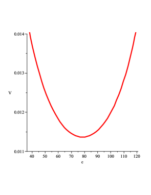
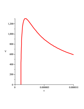
Figure 1: The volume as a function of the time variable $c$. We see a bounce occurring in the place where usual Kantowski–Sachs would have a singularity (left panel). The right panel shows the volume as a function of time close to the Kantowski–Sachs horizon ($b=0$), where the volume vanishes. Calculations use $M=5\times 10^{5}M_{\rm Planck}$.

In figure 2 we show the volume as a function of the “radial” variable $r^{2}=p_{c}$. The volume is multi-valued and it corresponds to the contracting and expanding phases. The rate at which the volume contracts depends on the value of $c_{0}$. We have chosen it here in such a way that the contracting and expanding rates are very close to each other. This, however, is a choice. In particular, the region where the holonomized theory departs from general relativity will change depending on such choice. If one chooses, as we did, a “symmetric” evolution, the region of departure is confined near the bounce in a symmetric way. Other choices can lead to the region extending far away from the bounce either into the future or the past of it. It is remarkable that no matter what choice of $c_{0}$ initially, the system will eventually go past the bounce and return to a regime where the holonomized theory approximates general relativity and a future horizon will develop with the same mass value. That is, the presence of both horizons and the bounce is robust. How the bounce occurs and when the holonomized theory starts and stops its departure from general relativity depends on the initial data. This is a reflection of the instabilities that were noticed in the recursion relations of the loop representation treatment of these models khanna .

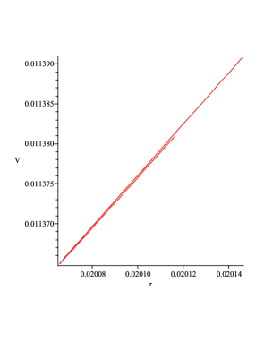
Figure 2: The volume as a function of the “radial” time variable $r^{2}=p_{c}$. It can be seen that it contracts till it achieves a minimum value, it then expands at the same expansion rate as it contracted. This is achieved if one chooses the initial data for $c_{0}$ at the horizon in such a way that the evolution is symmetric at the “bounce”. This, in particular implies that the region where the holonomized theory departs from general relativity is minimized. For other choices, the region of departure is larger.

Figure 3 shows the sine of $\mu b$ versus the time variable $c$. The sine of $\mu\,b$ divided by $\mu$ is the variable in the holonomized theory that replaces the connection $A_{\phi}$ in the usual theory. Both theories agree when the sine is small. We see that indeed the sine is small close to the horizons and maximal at the bounce. The time variable $c$ chosen is such that the region close to the “bounce” measured in terms of the radial variable is achieved very fast and lasts for a long “time”, therefore the sine of $\mu b$ is large through most of the evolution. One can see that when measured in terms of the volume the connection departs from it classical value close to bounce.

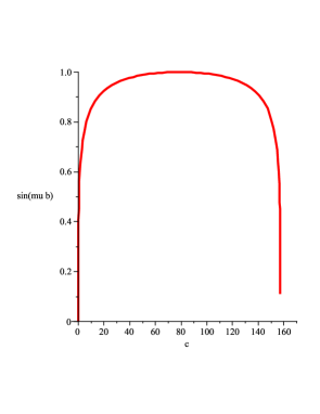
Figure 3: The sine of $\mu b$ vs $c$. When the sine is close to one the holonomized theory departs from general relativity significantly. We see that both theories agree at the initial and final moments, when the cosmological horizons are present. The diagram is symmetric in spite of its appearance, it is hard for the plotting program to numerically get to the points near the final horizon, since the points gather exponentially.

3.3 Quantum corrections

We have discussed the classical approximation. Let us now proceed to consider the quantum corrections, which involve the prefactor $A(b,c)$ in equation (27). We start by noting that the proposed solution for the wavefunction satisfies the boundary conditions implied by the kinematical Hilbert space. That is, $\Psi(-\pi/\mu,c)=\Psi(\pi/\mu,c)$, $\Psi(b,-\pi/\mu)=\Psi(b,\pi/\mu)$. We have required that the boundary conditions be periodic in $c$ and $b$ with period $2\pi/\mu$. It turns out that the only region of phase space of importance is between $0$ and $\pi/\mu$. In the other three regions one obtains the same $|\Psi|^{2}$ and the physical predictions are the same. It might appear surprising to impose boundary conditions in the variable $c$, which we are using as “time”. In principle one would think that specifying “future” boundary values would violate causality. Remarkably, this is not the case. The value of $c_{0}$ is arbitrary and the final result of the evolution is in no way determined by the periodicity imposed.

The dynamical Hilbert space is therefore given by arbitrary functions of the two constants of the motion $c_{0},M$. As the Schwarzschild external solution depends only of $M$ one can restrict the Hilbert space to the symmetric semi-classical solution around the bounce that are the ones whose behavior departs from the classical only close to radial distances of the order of Planck scale. Given $\mu$ this is equivalent to choose $c_{0}$ such that

$${c_{0}}=\frac{1}{\mu}\tan^{-1}\left[\frac{2\Theta^{2\Delta^{-1}}}{\Theta^{4\Delta^{-1}}-1}\right],$$ (36)

with

$$\Theta=\frac{{2}^{-\Delta/4}\left(2+\sqrt{2}\right)^{\Delta/2}}{\left(\sqrt{2}+2\Delta\right)\gamma^{2}\mu^{2}}\left(\left[-\sqrt{2}+4+2\,\Delta\right]\gamma^{2}\mu^{2}+\left(4-2\,\sqrt{2}\right)\left(1+\Delta\right)\right))$$ (37)

and $\Delta=\sqrt{1+\gamma^{2}\mu^{2}}$. Going to the full quantum theory, however, will not allow to choose precisely the values of $c_{0},M$ that correspond to the symmetric bounce, and one will have a spread implying that the region where the bounce occurs will be larger than the one we consider here in the symmetric case.

Finally, one can show that the evolution in $c$ is unitary. In fact one can see that $H_{\rm True}$ is self-adjoint by using the following technique porto4 : Check the dimensionality of the two subspaces: ${\cal K}_{+}={\rm ker}(H_{\rm True}+i)$ and ${\cal K}_{-}={\rm ker}(H_{\rm True}-i)$ They are self-adjoint if and only if both spaces have the same dimensionality. In this case the wavefunctions $\Psi$ multiplied by the exponential factor

$$\exp\left(\mp 4\,\tanh^{-1}\left({\frac{\cos\left(\mu\,{\it b}\right)\sin\left(\mu\,{\it c}\right)}{\gamma\mu\left({{\mu}^{2}{\gamma}^{2}+1}\right)}}\right)\right)$$ (38)

respectively belong to each kernel and are normalizable in the kinematical space. An important observation is in order here, the elements of the physical space $\Psi(b,c)$ are also normalizable with the inner product of the kinematical space and therefore they can be also used to define a relational evolution in terms of conditional probabilities, as for instance in the proposal of Page and Wootters PaWo ; njp . A detailed study of these definition of the evolution that do not require a deparametrization of the constraint will be given elsewhere.

We have therefore carried out a quantization of the interior of the Schwarzschild space-time using loop quantum gravity techniques. We have shown how the singularity is replaced by a bounce, and what conditions are needed for the bounce to occur in a regime of Planck energy. We have also outlined how one would construct the quantum theory for the model. It is interesting to compare the interior and exterior treatments. In the latter (and also in the complete space-time treatment of Kuchař kuchar ) one is left with an quantum theory in which wavefunctions are arbitrary functions mass of the space-time, which is conserved. Here, while treating the interior as a cosmology, we are left with arbitrary functions of an observable, which evaluated on the initial data is determined entirely by $c_{0}$. This is the variable conjugate to $p_{c}$, whose initial value is associated with the mass of the Schwarzschild space-time. Therefore the two pictures are clearly reconciled.

This work was supported in part by grant NSF-PHY-0554793, 9907949, 0456913, funds of the Hearne Institute for Theoretical Physics, The Eberly research funds of PennState, FQXi, CCT-LSU and Pedeciba (Uruguay).

References

- (1) M. Campiglia, R. Gambini and J. Pullin, Class. Quant. Grav. 24, 3649 (2007) [arXiv:gr-qc/0703135].
- (2) K. V. Kuchar, Phys. Rev. D 50, 3961 (1994) [arXiv:gr-qc/9403003].
- (3) M. Bojowald and R. Swiderski, Class. Quant. Grav. 23, 2129 (2006) [arXiv:gr-qc/0511108].
- (4) A. Ashtekar and M. Bojowald, Class. Quant. Grav. 23, 391 (2006) [arXiv:gr-qc/0509075].
- (5) L. Modesto, Int. J. Theor. Phys. 45, 2235 (2006) [arXiv:gr-qc/0411032].
- (6) C. G. Boehmer and K. Vandersloot, arXiv:0709.2129 [gr-qc].
- (7) A. D. Polyanin, V. F. Zaitsev, A. Moussiaux, “Handbook of first order partial differential equations”, Taylor and Francis, London, (2002). See also http://eqworld.ipmnet.ru/en/solutions/fpde/fpde2210.pdf
- (8) M. Bojowald, D. Cartin and G. Khanna, arXiv:0704.1137 [gr-qc] and references therein.
- (9) M. Reed and B. Simon, “Methods of Mathematical Physics Vol. II”, Academic Press, New York (1975); J. Weidmann, “Linear operators in Hilbert spaces” Springer Verlag, New York (1990).
- (10) D. N. Page and W. K. Wootters, Phys. Rev. D 27, 2885 (1983); W. Wootters, Int. J. Theor. Phys. 23, 701 (1984); D. N. Page, “Clock time and entropy” in “Physical origins of time asymmetry,” J. Halliwell, J. Perez-Mercader, W. Zurek (editors), Cambridge University Press, Cambridge UK, (1992).
- (11) R. Gambini, R. Porto, J. Pullin, New J. Phys. 6, 45 (2004) [arXiv:gr-qc/0402118].