Modeling disorder in graphene
Abstract
We present a study of different models of local disorder in graphene. Our focus is on the main effects that vacancies — random, compensated and uncompensated —, local impurities and substitutional impurities bring into the electronic structure of graphene. By exploring these types of disorder and their connections, we show that they introduce dramatic changes in the low energy spectrum of graphene, viz. localized zero modes, strong resonances, gap and pseudogap behavior, and non-dispersive midgap zero modes.
pacs:
71.23.-k,81.05.Uw,71.55.-iGraphene is poised to become a new paradigm in solid state physics and materials science, owing to its truly bi-dimensional character and a host of rich and unexpected phenomenaA.K.Geim and Novoselov (2007); Castro Neto et al. (2006, 2007). These have cascaded into the literature in the wake of the seminal experiments that presented a relatively easy route towards the isolation of graphene crystalsNovoselov et al. (2004).
Carbon is a very interesting element, on account of its chemical versatility: it can form more compounds than any other element Chang (1991). Its valence orbitals are known to hybridize in many different forms like , , , and others. As a consequence, carbon can exist in many stable allotropic forms, characterized by the different relative orientions of the carbon atoms. Carbon binds through covalence, and leads to the strongest chemical bonds found in nature. Common to the most interesting forms of carbon is the so-called graphene sheet, a single plane of carbon organized in an honeycomb lattice (Fig. 1). Graphite, for instance, is made of stackings of graphene planes, nanotubes from rolled graphene sheets, and fullerenes are wrapped graphene. Yet, for many years, it was believed that graphene itself would be thermodynamically unstable. This presumption has been overturned by a series of remarkable experiments in which truly bi-dimensional (one atom thick) sheets of graphene have been isolated and characterized Novoselov et al. (2004). This means that studies of the 2D (Dirac) electron gas can now be performed on a truly 2D crystal, as opposed to the traditional measurements made at interfaces as in MOSFET and other structures Novoselov et al. (2005a).
The crystalline simplicity of graphene — a plane of hybridized carbon atoms arranged in a honeycomb lattice — is deceiving. The characteristics of the honeycomb lattice make graphene a half-filled system with a density of states (DOS) that vanishes linearly at the neutrality point, and an effective, low energy quasiparticle spectrum characterized by a dispersion which is linear in momentumWallace (1949) close to the Fermi energy. These two features underlie the unconventional electronic properties of this material, whose quasiparticles behave as Dirac massless chiral electronsSemenof (1984). Consequently, many phenomena of the realm of quantum electrodynamics (QED) find a practical realization in this solid state material. They include: the minimum conductivity when the carrier density tends to zeroNovoselov et al. (2005b); the new half-integer quantum Hall effect, measurable up to room temperatureNovoselov et al. (2005b); Klein tunnelingKatsnelson and Novoselov (2007); strong overcritical positron-like resonances in the Coulomb scattering cross-section analogous to supercritical nuclei in QED Pereira et al. (2007); Shytov et al. (2007); the zitterbewegung in confined structuresPeres et al. (2006); anomalous Andreev reflectionsMiao et al. (2007); Beenakker et al. (2007); negative refraction Cheianov et al. (2007) in p-n junctions.
Arguably, the most interesting and promising properties from the technological point of view are its great crystalline quality, high mobility and resilience to very high current densitiesA.K.Geim and Novoselov (2007); the ability to tune the carrier density through a gate voltageNovoselov et al. (2004); the absence of backscatteringAndo and Nakanishi (1998) and the fact that graphene exhibits both spin and valley degrees of freedom which might be harnessed in envisaged spintronicKane and Mele (2005); Cho et al. (2007) or valleytronic devicesRycerz et al. (2007).
Disorder, ever present in graphene owing to its exposed surface and the substrates, is the central concern of this paper. In particular, we focus on the effects of vacancies and random impurities in the electronic structure of bulk graphene. The models examined below apply to situations in which Carbon atoms are extracted from the graphene plane (e.g. through irradiationEsquinazi et al. (2003)), in which adatoms and/or adsorbed species attach to the graphene planeSchedin et al. (2007), or in which some carbon atoms are chemically substituted for other elements. They are, therefore, models of local disorder. We do not consider explicitly other sources of disorder like rough edges or ripplesMeyer et al. (2007), or the dramatic effects of Coulomb impurities, which have been discussed elsewherePereira et al. (2007); Lewenkopf et al. (2007). In this article we expand the discussion of vacancies initiated in Ref. Pereira et al., 2006, using the same techniques, and discuss the consequences of local disorder originally presented in Ref. Pereira, 2006. Numerically we resort to exact diagonalization calculations and to the recursion methodHaydock et al. (1972, 1975). The latter allows the calculation of the DOS and other spectral quantities for very large system sizes with disorder. In our case, the calculations below refer to honeycomb lattices with carbon atoms, a size already of the order of magnitude of the real samples, if not larger for some experiments.
The article is organized as follows. In section I we present the basic electronic properties of electrons in the honeycomb lattice, mostly to introduce the notation and the details relevant for the subsequent discussions. In section II we present our results regarding the different models of disorder. This section is subdivided according to the different models of disorder studied: vacancies in II.1 and II.2, local impurities in II.3 and substitutional impurities in II.4. The discussion of the results is kept within each subsection and the principal findings of this paper are highlighted in the conclusion, in section III.
I Electrons in a Honeycomb Lattice
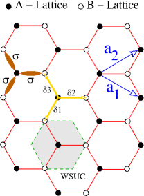
Graphene consists of carbon atoms organized into a honeycomb lattice, bonded through covalence between two orbitals of neighboring atoms (Fig. 1). The graphene plane is defined by the plane of the orbitals. The saturation of the resulting bonding orbitals, leaves an extra electron at the remaining orbital per carbon atom. Ideal graphene has therefore a half-filled electronic ground state.
The Bravais lattice that underlies the translation symmetries of the honeycomb lattice is the triangular lattice, whose primitive vectors and are depicted in Fig. 1. One of the consequences is the existence of two atoms per unit cell, that define two sublattices ( and in the figure): indeed, the honeycomb lattice can be thought as two interpenetrating triangular lattices. This bipartite nature of the crystal lattice, added to the half-filled band, imposes an important particle-hole symmetry as will be discussed later.
The electronic structure of graphene can be captured within a tight-binding approach, in which the electrons are allowed to hop between immediate neighbors with hopping integral eV, and also between next-nearest neighbors with an additional hopping :
| (1) |
The presence of the second term introduces an asymmetry between the valence and conduction bands, thus violating particle-hole symmetry. To emphasize the two sublattice structure of the honeycomb, we can write the Hamiltonian as
| (2) |
with operators and pertaining to sublattices and respectively. The vectors connect atom to its immediate neighbors, whereas the connect atom to its six second neighbors. Fourier transforming eq. (2) and introducing a spinor notation for the sublattice amplitudes leads to
| (3) |
Since the spin degree of freedom does not play a role in our discussion other than through a degeneracy factor, it will been omitted, for simplicity. The functions and read
| (4) | |||
| (5) |
where alone is the dispersion relation of a triangular lattice, and yield, after diagonalization of (3), the dispersion relations for graphene:
| (6) |
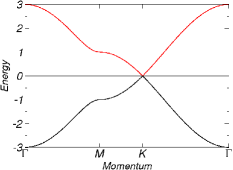
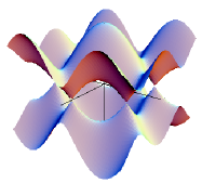
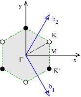
The two bands are represented in Fig. 2 in the domain . This unusual bandstructure makes graphene very peculiar with valence and conduction bands touching at the Fermi energy, at a set of points at the edge of the first Brillouin zone, equivalent to the points and by suitable reciprocal lattice translations. Its low energy physics is dictated by the dispersion around those two inequivalent points, which turns out to be linear in . In fact, expanding (5) around either
| (7) |
one gets the so-called effective bandstructureWallace (1949):
| (8) |
with a Fermi velocity, (, and we take units in which and ). When the dispersion is purely conical, as in a relativistic electron in 2D. For this reason, the two cones tipped at and are known as Dirac cones. The low-energy, continuum limit of (2) is given by
| (9) |
where is a two dimensional spinor obeying the Dirac equation in 2D González et al. (1992).
In panel 2 the band dispersion is plotted along the symmetry directions of the BZ indicated in Fig. 1, and in panel 3 the DOS for different values of the nearest-neighbor hopping, , are plotted. Focusing on the particle-hole symmetric case (), it is clear that, besides the marked van Hove singularities at , the most important feature is the linear vanishing of the DOS at the Fermi level, a fact that is at the origin of many transport anomalies in this material Peres et al. (2005); Castro Neto et al. (2007).
Particle-hole symmetry in this problem arises from the bipartite nature of the honeycomb lattice, and is a general property of systems whose underlying crystal lattice has this nature. When we have a bipartite lattice, the basis vectors of the Hilbert space can be ordered so that, for any ket, , the amplitudes in sublattice come first. For example, if are the Wannier functions for the orbitals in sublattice , and the ones in sublattice , then our ordered basis could be . If the Hamiltonian includes hopping only between nearest neighbors, this means that it only promotes itinerancy between different sublattices. The stationary Schrödinger equation then reads, in matrix block form in the ordered basis,
| (10) |
Expanding we get
| (11) |
and therefore, if is an eigenstate, so is . For a half-filled system, the elementary excitations around the Fermi sea can be thought, as usual, as particle-hole pairs. Since in that case , particles and holes have symmetric dispersions. This is completely analogous to the situation found in simple semiconductors or semimetals, although matters are slightly more complicated in graphene because there are two degenerate points, and in the BZ. Thus there will be two families of particle and hole excitations: one associated with the Dirac cone at , and the other with the cone at , like in a multi-valley semiconductor.
II Local Disorder in Graphene
Disorder is present in any real material, graphene being no exception. In fact, true long-range order in 2D implies a broken continuous symmetry (translation), which violates the Hohenberg-Mermin-Wagner theorem Mermin and Wagner (1966); Hohenberg (1967). So, by this reason alone, defects must be present in graphene and, in a sense, as paradoxical as it might sound, are presumably at the basis of its thermodynamic stability.
But the study of disorder effects on graphene is motivated by more extraordinary experimental results. One of them is the study undertaken by Esquinazi et al. (2003) in which highly oriented pyrolytic graphite (HOPG) samples were irradiated via high energy proton beams. As a result, the experiments revealed that the samples acquired a magnetic moment, displaying long range ferromagnetic order up to temperatures much above K. This triggered enormous interest, since the technological possibilities arising from organic magnets are many and varied. Furthermore, carbon, being the most covalent of the elements, has a strong tendency to saturate its shell in its allotropes, and is somehow the antithesis of magnetism. Besides the moment formation, it was found that the magnitude of the saturation moment registered in hysteresis curves was progressively increased with successive irradiations. This is strong evidence that the defects induced by the proton beam are playing a major role in this magnetism. In this context the study of defects and disorder in graphene gains a significant pertinence.
In the following paragraphs we will unveil some details and peculiarities that emerge from different models of disorder applied to free electrons in the honeycomb lattice.
II.1 Vacancies
Vacancies are one of the defects more likely to be induced in the graphene structure by proton irradiation. A vacancy is simply the absence of an atom at a given site. When an atom is removed two scenarios are possible: either the disrupted bonds remain as dangling bonds, or the structure undergoes a bond reconstruction in the vicinity of the vacancy, with several possible outcomes Ding (2005). In either case, a slight local distortion of the lattice is expected. In the following discussion, however, it is assumed that, as first approximation, the creation of a vacancy has the sole effect of removing the orbital at a lattice point, together with its conduction band electron. In this sense, the physics of the conduction band electrons is still described by the Hamiltonian (1), where now the hopping to the vacancy sites is forbidden.
II.1.1 Vacancies and a theorem
Vacancies have an interesting consequence when . If the distribution of vacant sites is uneven between the two sublattices, zero energy modes will necessarily appear. This follows from a theorem in linear algebraBrouwer et al. (2002) and can be seen as follows. Assume, very generally, that we have a bipartite lattice, with sublattices and (It can be any bipartite lattice like the square or honeycomb lattices in 2D, cubic in 3D, etc.), and that the number of orbitals/sites in () is (). Just as we did before, the basis vectors of the Hilbert space can always be ordered so that any ket, , has the amplitudes on sublattice appearing first, followed by the amplitudes on sublattice :
| (12) |
We now consider an Hamiltonian containing only nearest-neighbor hopping, plus some local energy () on each sublattice. The corresponding stationary Schrödinger equation will then be (in matrix block form that respects the ordering of the basis)
| (13) |
where is the identity matrix, a matrix, and () a vector in a subspace of dimension ().
To analyze the spectrum we note that
| (14) |
which, from cross-substitution, implies that
| (15) |
If we call to the (non-negative) eigenvalues of , the spectrum of is then
| (16) |
The symmetry about simply reflects the particle-hole symmetry.
II.1.2 Uncompensated lattices
States of a peculiar nature should appear when the number of sites in each sublattice is different. Without any loss of generality we take . Since the block in (13) is a linear application from a vector space having , onto a vector space with , it follows from basic linear algebra that
-
•
;
-
•
has no solutions other than the trivial one;
-
•
has non-trivial solutions that we call .
From the rank-nullity theorem,
| (17) |
and hence the null space of has dimension: . Consequently, there are states of the form
in which satisfies , that are eigenstates of with eigenvalue :
| (18) |
Furthermore, since implies the existence of linearly independent , this eigenstate has a degeneracy of . It should be stressed that a state of the form has only amplitude in the sublattice. Therefore, we conclude that, whenever the two sublattices are not balanced with respect to their number of atoms, there will appear states with energy , all linearly independent and localized only on the majority sublattice. In addition, one can modify sublattice in any way (remove more sites, for instance) that these zero modes will remain totally undisturbed.
We remark that in the above the details of the hopping matrix were not specified and need not be. The result holds in general, provided that the hopping induces transitions between different sublattice only, and that the diagonal energies are constant (diagonal disorder is excluded).
II.1.3 Zero modes
The case with is of obvious relevance for us, since our model for pristine graphene does not include any local potentials. In this situation, the above results imply that introducing a vacancy in an otherwise perfect lattice, immediately creates a zero energy mode. Now this is important because those states are created precisely at the Fermi level, and have this peculiar topological localization determining that they should live in just one of the lattices.
Even more interestingly, it is possible to obtain the exact analytical wavefunction associated with the zero mode induced by a single vacancy in a honeycomb lattice. This was done by the authors and collaborators in Ref. Pereira et al., 2006, and will not be repeated here. We only mention that the wavefunction can be constructed by an appropriate matching of the zero modes of two semi-infinite and complementary ribbons of graphene, and that, in the continuum limit, the wavefunction of the zero mode introduced by one vacancy has the formPereira et al. (2006)
| (19) |
The important point is that the amplitude of this state decays with the distance to the vacancy as , and thus has a quasi-localized character, although strictly not-normalizable. And such quasi-localized state appears exactly at the Fermi level.
Should another vacancy be introduced in the same sublattice, we already know that another zero mode will appear. However, the nature of the two zero modes will depend whether the vacancies are close or distant. In the latter case, the hybridization between the two modes should be small on account of the decay, and we can expect two states of the form (19) about each vacancy site. Of course significant effects in the thermodynamic limit can only arise with a finite concentration of vacancies, and for such analysis we undertook the numerical calculations described next.
II.1.4 Numerical Results – Single Vacancy
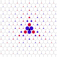
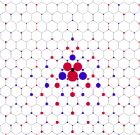
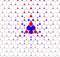
The first calculation is the numerical verification of the exact analytical result for the localized state in (19). For that, we consider the tight-binding Hamiltonian (1) and calculate numerically, via exact diagonalization, the full spectrum and eigenstates in the presence of a single vacancy. For some typical results we turn our attention to Fig. 4. There we plot a real-space representation of some selected wavefunctions. This has been done by drawing a circle at each lattice site, whose radius is proportional to the wavefunction amplitude at that site, and whose color (red/blue) reflects the sign (+/-) of the amplitude at each site. Thus bigger circles mean higher amplitudes. In the first panel, 4, we are showing the eigenstate with lowest, yet non-zero, absolute energy. It is visible that the wavefunction associated with such state spreads uniformly across the totality of the system. like a plane wave. In the second panel, 4, we draw the wavefunction of the state , that corresponds to (19). The state is clearly decaying as the distance to the central vacancy increases. In addition, the state exhibits the full point symmetry about the vacant site, just as expected. This picture provides a snapshot of the lattice versionPereira et al. (2006) of (19). Since only one vacancy was introduced, the state shown in Fig. 4 is the only zero mode present.
When particle-hole symmetry is disturbed by a non-zero , we still find states having this quasi-localized nature, where the wavefunction amplitude is still quite concentrated about the vacancy. Two examples are shown in panels 4 and 4. They are two eigenstates with neighboring energy calculated for the same system. An important difference occurs here, in that, unlike the case where only one localized state appears, the particle-hole asymmetric case opens the possibility for more than one of such states.
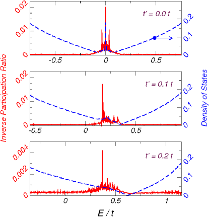
This fact can be seen more transparently through the inverse participation ratio (IPR) of the eigenstates. With such purpose in mind, the IPR
was calculated across the band in both the and cases, with a single central vacancy. Typical results are shown in Fig. 5.
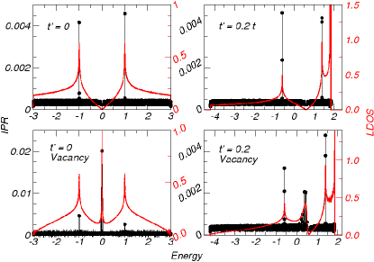
From 5 we do confirm that, when , the presence of a vacancy introduces a localized state at , which is reflected both by the enhanced IPR there, and by the sharply peaked LDOS calculated at the vicinity of the vacancy site. Although not shown in this figure, the amplitude of the peak in the LDOS at , , decays as the distance between and the vacancy increases, in total consistence with the analytical picture. When next-nearest neighbor hopping is included, we also confirm the appearance of states with a considerably enhanced IPR. Not only that, but, instead of one, we do observe a set of states with IPR much larger than the average for the remainder of the band. The LDOS is also enhanced near these energies, although the effect appears as a resonance on account of the finite DOS, in contrast with the sharp peak in the previous, particle-hole symmetric, case.
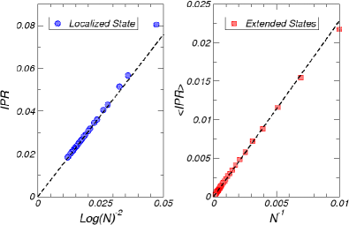
A more definite and quantitative analysis is provided by the results in the subsequent panel (Fig. 5). Here we present the dependence of on the number of carbon atoms in the system, . To understand the differences, we recall that the IPR for extended states should scale as
| (20) |
But, for the zero mode (it should be obvious that when the term zero mode is employed, we are referring to the case with .), we face an interesting circumstance. Remember that the wavefunction (19) is not normalizable. So, strictly speaking, the state is not localized, and hence the designation quasi-localized that we have adopted above. The consequence of this is that the normalization constant for depends on the system size:
| (21) |
This, in turn has an effect on the IPR because is defined in terms of normalized wavefunctions:
| (22) |
This scaling of the IPR with is precisely the one obtained numerically in Fig. 5 (left) for the zero mode, and is just another way of confirming the decay of this wavefunction.
II.1.5 Numerical Results – Finite Concentration of Vacancies
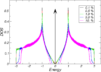
Unlike the single vacancy case, the dilution of the honeycomb via the introduction of a finite concentration of vacancies is not solvable using the analytical expedients employed in ref. Pereira et al., 2006, and numerical calculations become essential in this case. Our procedure consists in diluting the honeycomb lattice with a constant concentration of vacancies, which we call (). The diluted sites are chosen at random and the global DOS, averaged over several vacancy configurations, is calculated afterwards. This is clearly a disordered problem, and we employ the recursive method allowing us to obtain the DOS for systems with sites (which is already of the order of magnitude of the number of atoms in real mesoscopic samples of graphene studied experimentally). Some results are summarized in Fig. 6.
One of the effects of this disorder is, as always, the softening of the van-Hove singularities (not shown). But the most significant changes occur in the vicinity of the Fermi level (Fig. 6). In the presence of electron-hole symmetry (), the inclusion of vacancies brings an increase of spectral weight to the surroundings of the Dirac point, leading to a DOS whose behavior for mostly resembles the results obtained elsewhere within coherent potential approximation (CPA) Peres et al. (2005). Indeed, for higher dilutions, there is a flattening of the DOS around the center of the band just as in CPA. The most important feature, however, is the emergence of a sharp peak at the Fermi level, superimposed upon the flat portion of the DOS (apart from the peak, the DOS flattens out in this neighborhood as is increased past the shown here). The breaking of the particle-hole symmetry by a finite results in the broadening of the peak at the Fermi energy, and the displacement of its position by an amount of the order of . All these effects take place close to the the Fermi energy. At higher energies, the only deviations from the DOS of a clean system are the softening of the van Hove singularities and the development of Lifshitz tails (not shown) at the band edge, both induced by the increasing disorder caused by the random dilution. The onset of this high energy regime, where the profile of the DOS is essentially unperturbed by the presence of vacancies, is determined by , with being essentially the average distance between impurities.
To address the degree of localization for the states near the Fermi level, the IPR was calculated again, via exact diagonalization on smaller systems. Results for different values of are shown in Fig. 6 for random dilution at . One observes, first, that for all energies but the Fermi level neighborhood, as expected for states extended up to the length scale of the system sizes used in the numerics. Secondly, the IPR becomes significant exactly in the same energy range where the DOS exhibits the vacancy-induced anomalies discussed above. Clearly, the farther the system is driven from the particle-hole symmetric case, the weaker the localization effect, as illustrated by the results obtained with . To this respect, it is worth mentioning that the magnitude of the strongest peaks in at and is equal to the magnitude of the IPR calculated above for a single impurity problem. Such behavior indicates the existence of quasi-localized states at the center of the resonance, induced by the presence of the vacancies. For higher doping strengths, the enhancement of is weaker in the regions where the DOS becomes flat. This explains the qualitative agreement between our results and the ones obtained within CPA in that region, since CPA does not account for localization effects.
In summary, in this section, we saw that a single vacancy introduces a quasi-localized zero mode. Its presence is ensured by the uncompensation between the number of orbitals in the two sublattices, and a theorem from linear algebra. The presence of this mode translates in the appearance of a peak in the LDOS near the vacancy, and in an enhanced IPR for this state. When we go from one to a macroscopic number of vacancies, we saw that both the peak and the enhancement of the IPR persist in the global DOS at .
II.2 Selective Dilution
It is important to recall that the results of the previous section pertain to lattices that were randomly diluted. During such process, we expect the number of vacancies in sublattice to be equal to the number of vacancies in sublattice , on average. Strictly speaking, since our original lattices are always chosen with , the fluctuations on the degree of uncompensation, , should scale as thus vanishing in the thermodynamic limit. Because of this, in principle, we would expect the lattices used above to be reasonably compensated. But the theorem in § II.1.1 only guarantees the presence of zero modes when the lattice is uncompensated. It turns out that, notwithstanding our utilization of rather large system sizes, such fluctuations are still significant and the lattices were indeed slightly uncompensated.
This clearly begs the clarification of the origin of the zero modes in the cases with finite densities of vacancies. Do they appear only through these fluctuations in the degree of sublattice compensation, or can we have zero modes even with full compensation? To try to elucidate this we developed a controlled approach to this issue, in the following. From now on we consider only the particle-hole symmetric situation ().
II.2.1 Complete uncompensation
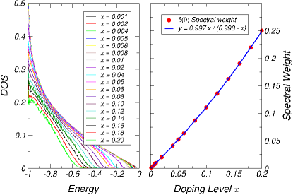
We have studied the DOS for systems in which only one of the sublattices was randomly diluted, with a finite concentration of vacancies. In this case, the system has precisely a number of zero modes that equals the number of vacancies. Starting from a clean lattice with sites, the latter corresponds to . We should thus expect a peak contributing to the global DOS, with an associated spectral weight, that coincides with the fraction of zero modes:
| (23) |
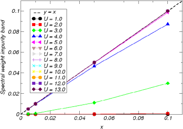
Since the total spectral weight is normalized to 1, the spectral weight at has to be transferred from the states in the band. In Fig. 7 we show what is happening. As seen in 7, the selective dilution promotes the appearance of a gap in the DOS, whose magnitude increases with the amount of dilution. At the center of the gap we can only see an enormous peak (not visible in the range used) staying precisely at , corroborating our expectations regarding the Dirac-delta in the DOS. But since it appears exactly at , we cannot resolve numerically its associated spectral weight. To obtain such spectral weight we calculated the spectral weight loss in the remainder of the band. The result and its variation with the amount of dilution, , is displayed in the right-most frame of Fig. 7. A non-linear fit to the data reveals that the dependence expected from (23) is indeed verified by the accord between the fitted curve in Fig. 7 and eq. (23).
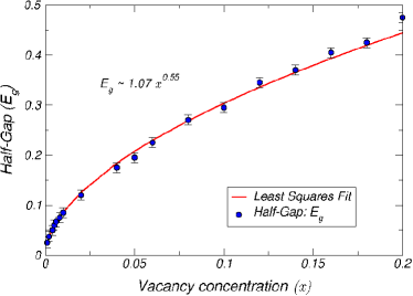
As Fig. 7 shows, the spectral weight is transferred almost entirely from the low energy region near and from the high energy regions at the band edges. This depletion near introduces the gap, . A gap implies the existence of a new energy scale in the problem. Since the hopping is the only energy scale in the Hamiltonian, such new scale has to come from the concentration of vacancies. By dimensional analysis, such scale is dictated essentially by the average distance between vacancies ()
| (24) |
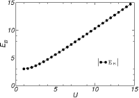
When the the magnitude of the gap found numerically is plotted against we arrive at the curve of Fig. 8. The least squares fit shown superimposed onto the numerical circles leaves confirms this assumption, and we arrive at a quite interesting situation, of having a half-filled, particle-hole symmetric and gapped system, with a finite concentration of (presumably quasi-localized) zero modes at the mid-gap point.
II.2.2 Controlled uncompensation
We now turn to a more controlled approach to the dilution and uncompensation. For that we introduce an additional parameter, , that measures the degree of uncompensation. As before, we want to study finite concentrations of vacancies. This is determined by in such a way that the number of vacancies in a lattice with sites will be . But now, the number of vacancies in each sublattice is determined by
| (25) |
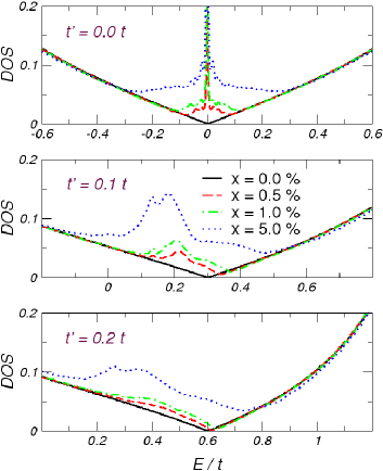
with . Therefore, the parameter permits an interpolation between completely uncompensated dilution (), and totally compensated dilution (). Let us look directly at the results for the DOS, calculated at different and , and plotted in Fig. 9.
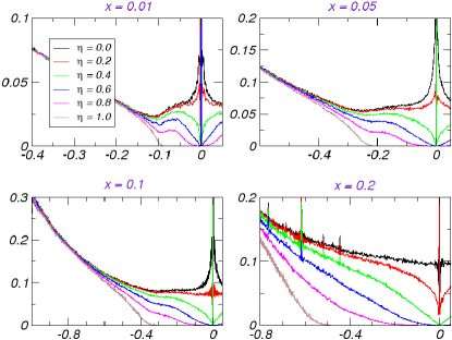
At any concentration the following sequence of events unfolds as decreases from 1 to 0: (i) There is a perfectly defined gap in the limit discussed above; (ii) for a small hump develops at the same energy scale of the previous gap; (iii) although the gap seems to disappear, it is clearly visible that when , the DOS decays to zero after the hump in a pseudo-gap like manner, and is zero at ; (iv) decreasing further towards complete compensation (say, for ), this behavior persists, being visible that the DOS drops to zero at ; (v) closer to full compensation () the DOS seems to display an upward inflection near , and apparently does not drop to zero. Unfortunately, we are unable to resolve this region numerically with the desired accuracy. For instance, at higher dilutions we can still see the curve of dropping to zero near .
Naturally that, for all the cases with , the existence of zero modes is guaranteed. As before, we inspected this by calculating the missing spectral weight in the bands, and confirmed that it does agree with the fraction of uncompensated vacancies. Hence, the picture emerging from these results seems to suggest that, although the gap disappears for , the DOS still drops to zero at , and might drop in a singular way as approaches zero. If we separate the contributions of the zero modes to the global DOS from the contribution of the other states, the consequence of this would be that, in a compensated lattice (), the DOS associated with the other states would seem to diverge as , but would be zero precisely at . Stated in another way, coming from high energies, we would see a decreasing DOS up to some typical energy , at which point it would turn upwards. At very small energies the DOS would seem to be diverging but, at some point arbitrarily close to , it would drop precipitously down to zero. Unfortunately, at the moment the numerical calculations are not so accurate as to allow the confirmation or dismissal of such possibility. In fact, the peaks for are of the same magnitude of the ones found when the dilution is completely random across the two sublattices (Fig. 6). So, although the evidence is compelling towards the affirmative, these results are still inconclusive as to whether the zero modes disappear in a perfectly compensated diluted lattice or not.
II.3 Local Impurities
Vacancies are local scatterers in the unitary limit. A vacancy can be thought as an extreme case of a local potential, , when . In this context we investigated the intermediate case characterized by a finite local potential. The Hamiltonian in this case changes from the pure tight binding in (1) to
| (26) |
The first term represents the local potential of magnitude at the impurity sites . These impurity sites belong to the underlying honeycomb lattice but their space distribution is random. The concentration of impurities, , is kept constant and we consider only the case with in the sequel.
Physically the model summarized in the Hamiltonian of eq. (26) could describe the situation in which some of the carbon atoms are substituted by a different species. Another realistic circumstance has to do with the fact that a real graphene sheet is expected to have some molecules from the environment adsorbed onto its surfaceSchedin et al. (2007). Consequently, even if the honeycomb lattice of the carbon atoms is not disrupted with foreign atoms, the presence of adsorbed particles can certainly induce a local potential at the sites where they couple to the carbon lattice.
Much of the details of this model can be understood from the local environment around a single impurity, in which case exact results and closed formulas are obtainable within a T-matrix approachElliot et al. (1974). Hence, we start by analyzing the single impurity problem in the honeycomb lattice, taking into account the full electronic dispersion and calculating the exact local Green’s functions, which allow the identification of the main spectral changes introduced by the scattering potential.
Within T-matrix, the electron Green’s function is written as
| (27) |
In the Dyson-like expansion above is the non-interacting Green’s function whose matrix elements are denoted by (sub/superscripts refer to position/sublattice), and the T-matrix, , is formally defined in terms of the scattering potential, , byElliot et al. (1974); Doniach and Sondheimer (1999)
| (28) |
Taking for a potential localized only on site of sublattice A, the local Green’s function on that site reads
| (29) |
The function is simply related to the density of states per carbon atom in the absence of impurity, , through
| (30) |
The knowledge of suffices for the determination of on account of the analytical properties of and the Kramers-Kronig relations. Moreover, any new poles of the exact Green’s function can come only from the denominator in (29), and are determined by the condition
| (31) |
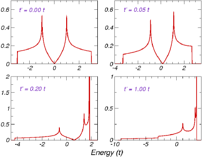
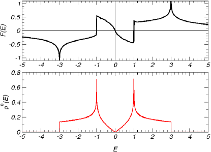
Should this condition be satisfied for within the branch cut of , the new poles will signal the existence of resonant states in the band, and bound states of the local potential otherwise. Since is known exactlyHanisch et al. (1995) (cfr. Fig. 3), so can be through eq. (30). The function is shown in Fig. 10. The profile of this function and the condition above, allows two immediate conclusions without further calculation: (i) the presence of the local potential induces bound states beyond the band continuum and (ii) a resonance appears at low energies beyond a certain threshold, , with energy of opposite sign with respect to the scattering potential, and which moves toward as .
The latter characteristic is certainly more interesting and we explore it a little further. To that extent notice that from (29) and (30) follows the interacting LDOS at the impurity site:
| (32) |
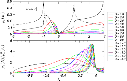
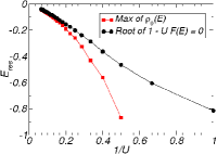
This quantity was calculated using the results of Fig. 10 and (32) and, at the same time, using the recursive method that we have been using so far. The two do coincide, just as expected since the solution of the single impurity problem is exact, and, on the other hand, the recursive method is exact for the particular case of the LDOSHaydock et al. (1972). The LDOS at the site of the impurity is shown in the top frame of Fig. 11 for several values of . The bottom frame shows the same data divided by the non-interacting DOS, which amounts to replacing by unity in the numerator of eq. (32). The resonance alluded above is visible in both panels through the marked enhancement of the LDOS in the vicinity of the Dirac point. The position of the maximum in differs slightly from the roots of eq. (31) due to the modulation introduced by in (32). This effect is shown in detail in Fig. 12 where the two values are explicitly compared. In addition, the LDOS also exhibits the Dirac-delta peak associated with the bound state (not shown in the figure), whose energy is plotted in Fig. 12 as a function of .
It is worth mentioning that analytical expressions can be obtained for the resonant condition (31) using the low energy Dirac approximation to the electronic dispersionPeres et al. (2005); Skrypnyk and Loktev (2006).
Returning now to our initial goal of populating the lattice with a finite concentration of local impurities, we expect the main features of the above analysis to hold to a large extent. But new features should also emerge from the possibility of multiple scattering and interference effects in a multi-impurity environment. Although some of these effects can be captured within standard approximations to impurity problemsDoniach and Sondheimer (1999), we choose to present the exact numerical results obtained with the recursion technique. Examples of such calculations are shown in Fig. 13, where the global DOS averaged over several configurations of disorder is shown for different potential strengths and concentrations.
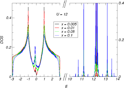
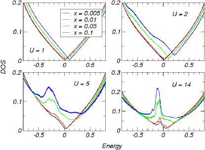
The presence of the local term clearly destroys the particle-hole symmetry, leading to the asymmetric curves in the figure. As Fig. 13 makes clear, among the features seen locally for a single impurity (Fig. 11), the ones that carry to the global DOS of the thermodynamic system with a finite concentration of impurities are the resonant enhancement of the DOS in the vicinity of the Dirac point, and the high energy features that dominate beyond the band edge, and are associated with the impurity states. One verifies that a finite concentration, , generates a sort of impurity band at scales of the order of , in accordance with the results in Fig. 12. This impurity band has an interesting splitted structure as can be seen in the figure and is completely detached from the main band for . In Fig. 13, we amplify the low energy region and display what happens as and vary. At small and the the DOS changes only through a simple translation of the band with the concomitant shift in the Dirac point, . This rigid shift of the band at low disorder is simply a consequence of the rigid band theoremKittel (1963): it states that the form of the DOS in an alloy system does not change with alloying, other than via a simple translation as given by first-order perturbation theory. In our case the magnitude of this shift is given by
| (33) |
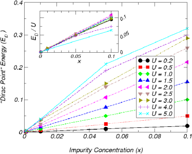
where an average over disorder is implied. We can confirm that the exact numerical results satisfy quantitatively this expectation by inspection of the data in Fig. 14. There we plot the position of the minimum in the DOS, , for several and , being evident that, for the concentrations analyzed, the relation (33) is quite accurately satisfied up to .
For local potentials higher than the rigid shift of breaks down and, in fact, the position of becomes slightly ill defined. We point out that concurrently with the shift of (and the band), there is a marked increase in the DOS at , unlike the single impurity case (cfr. Fig. 11). This, again, is expected and appears already in approximate methods like the CPA approximationPeres et al. (2005). Nonetheless, whereas shifts linearly for moderate potential strengths, the position of the resonance does not vary significantly with concentration, and is only enhanced with an increasing number of impurities (Fig. 13).
Another noteworthy aspect of this model has to do with the impurity band that emerges at high energies. Besides the effects just described, a change in the concentration of impurities implies a concomitant redistribution of spectral weight between the main band and the impurity band. This is plainly shown in Fig. 14 which displays the spectral weight in the impurity band against the concentration of impurities. This spectral weight is calculated by integrating the DOS in the region . As the figure shows, for the spectral weight of the impurity band saturates at the value , signaling the detachment of the impurity states from the main band. For those cases the spectral weight coincides with the concentration . It certainly had to be so because with increasing the impurity band drifts to higher energies, eventually disappearing from the problem in the unitary limit. As discussed previously in section II.1, the spectral weight of the main band is decreased by precisely , in the presence of a concentration of vacancies of . This is totally consistent with the fact that the local impurity interpolates between the clean case and the vacancy limit.
Finally, is also clear how the vacancy limit () emerges from the data in Fig. 13 as the resonance approaches and becomes more sharply defined. At the same time, the impurity band is displaced toward higher and higher energies, eventually projecting out of the problem in the vacancy limit.
II.4 Non-Diagonal Impurities
Another effect expected with the inclusion of a substitutional impurity in the graphene lattice is the modification of the hoppings between the new atom and the neighboring carbons. This happens because the host and substituting atoms have different radii, because the nature of the orbitals involved in the conduction band is different, or, most likely, a combination of both. Customary impurities in carbon allotropes are nitrogen, working as a donor, and boron, working as an acceptor Kaiser and Bond (1959). In fact, the selective inclusion of nitrogen and/or boron impurities in carbon nanotubes is a current practice in the hope to tune the nanotubes’ electronic response R. Droppa et al. (2004); Ciraci et al. (2004); Nevidomskyy et al. (2003).
In general the study of a perturbation in the hopping is much less studied in problems with impurities than the case of diagonal, on-site, perturbations. In the context of our investigations, the perturbation in the hopping can, again, be interpreted as an interpolation between a vacancy and an impurity. To be more precise, let us introduce the relevant Hamiltonian:
| (34) |
In this case, only nearest neighbor hopping is considered. Without the second term, above is the Hamiltonian for pure graphene. The last sum is restricted to the impurity sites, , and represents a perturbation in the hopping amplitude to its neighbors. Is plain to see that, when , all the impurity sites turn into vacancies since the hopping thereto is zero. As a result of that, this model provides another type of interpolation between pure graphene and diluted graphene. An important difference is that this model can be disordered when the impurities are placed at random, without breaking particle-hole symmetry, and, in this sense, is qualitatively much different from the case of local disorder discussed in the preceding section.
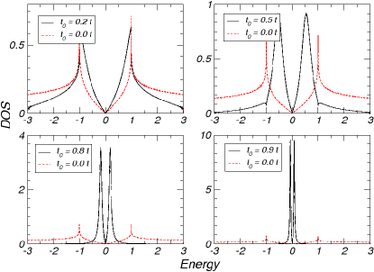
We first look at the LDOS in Fig. 15, which contains typical results for the local DOS near the impurity, and at the impurity site itself. Irrespective of whether the LDOS is calculated at or near the impurity, the resulting curves display a strong resonance in the low energy region, no bound states are formed and the curves are symmetrical with respect to the origin. As increases from zero, two simultaneous modifications in these resonances take place. The first is that they are clearly enhanced as approaches . The second is its shift in the direction of the Dirac point, in such a way that, when , the peak is already very close to . With regard to this last point, we systematically investigated the variation of the peak position in the LDOS at the impurity site with the value of .
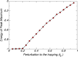
This dependence, which can be seen in Fig. 16, is approximately linear and, for , is reasonably well approximated by the linear function . The apparent saturation for smaller is due to the proximity to the van Hove singularity. The study of a single substitutional impurity has been also undertaken in ref. Peres et al., 2007, with identical results.
The double-peak structure close to the Dirac point can be qualitatively understood from the results regarding a vacancy. Suppose that one completely severs the hopping between a given atomic orbital and its immediate neighbors (i.e: set ). In this case we are left with an isolated orbital with energy and a vacancy in the honeycomb lattice, which we know also has a zero energy mode. If now is changed slightly, it will cause the hybridization of the two zero energy modes with the consequent splitting of the energy level, and hence the double peaked structure of the LDOS close to the Dirac point.
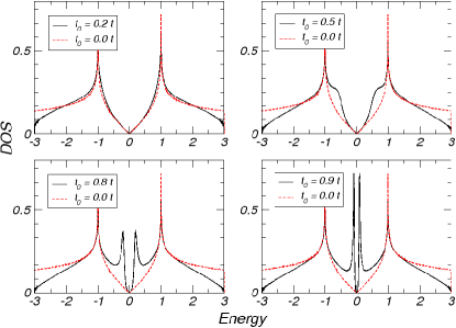
When we go from one impurity to a finite density of impurities, , we obtain a measurable influence in the thermodynamic limit. Our method in this case, consists in placing impurities at random positions in the lattice, keeping their concentration constant. The global DOS, averaged over several realizations of disorder, is presented in Fig. 17.
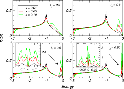
For intermediate values of , the perturbation in the hopping induces a resonance appearing at roughly the same energies as the ones found in Fig. 16. The resonance is enhanced at higher concentrations of impurities, and becomes more sharply defined as . Interestingly, as can be seen in the last panels of Fig. 17 and its inset, the resonant peak splits at higher perturbations. This splitting depends on the concentration of impurities being more pronounced for larger concentrations and is a new feature introduced by the finite number of impurities. As happened already in the case of local impurities, the exact numerical results have qualitative and quantitative features that could not be anticipated from calculations with a single impurity within the usual approximation methods. We would also like to point out the fact that, from inspection of the above figures, the DOS remains zero at , notwithstanding the sharp resonances in its vicinity. Since this model of disorder interpolates between clean graphene and graphene with vacancies, we are led to a situation similar to the one encountered in sec. II.2 for uncompensated vacancies. As before, it seems that, as the vacancy limit is approached, the DOS remains zero at the Fermi energy, despite diverging arbitrarily close to this point, and so the question of the DOS exactly at for vacancies lingers. Furthermore, unlike what happens with local impurities, there is no impurity band nor any high energy features appearing as : the action is all on the low energy regions. Strictly speaking, in the limit , the impurity sites become isolated from the carbon network. Hence those sites have to be removed from the Hilbert space for a meaningful physical description of the vacancy case as the limit (for local impurities the removal of the impurity sites is akin to the drift of the impurity band to infinity, carrying the spectral weight associated with the number of the impurities, which projects out of the problem).
Before closing, just a comment on the physical origin of this perturbation. In effect, the presence of a substitutional impurity like or will introduce, simultaneously, a perturbation in the hopping, and in the local energy. However, it is more or less clear from the discussions in the previous section that the clearest resonances near occur when the local potential, , is moderate or high, which is not the case for boron or nitrogen substituents. Hence, the perturbation in the hopping should perhaps be more significant in dictating the changes in the low-energy electronic structure in the real physical system.
III Conclusions
In this paper we have studied the influence of local disorder in the electronic structure of graphene, within the tight-binding approximation of eq. (1). We focused on vacancies in an otherwise perfect graphene plane and the not so extreme cases of local (diagonal) impurities and substitutional (non-diagonal, or both) impurities. In all cases we saw that disorder brings dramatic alterations of the spectrum in the vicinity of the Fermi level. This is highly significant since many of the peculiar physical properties of graphene stem from the vanishing of the DOS at the Dirac point.
In the case of vacancies, the DOS features a strong divergence at and close to , which is associated with the formation of quasi-localized states decaying as around the vacancies, which remain even in the presence of next-nearest neighbor hopping. Rather interesting is the particular case of lattices with uncompensated vacancies, in which case we found the appearance of a gap at low energies proportional to the concentration , and the coexistence of localized zero modes in the middle of this gap. For the extreme limit of dilution among sites of a given sublattice only, we showed that the gap is robust, and that a macroscopic number of quasi-localized zero modes dominates the spectral density in the middle of the gap. Moreover, these zero modes are strictly non-dispersive as imposed by symmetry, and give a contribution to the gapped DOS. This is very interesting, in particular if one reasons in terms of magnetic instabilities and formation of local magnetic moments. Such states might be at the origin of local magnetic moments, which would explain the magnetism seen experimentally in the irradiation experimentsEsquinazi et al. (2003).
We showed how the vacancy case emerges as the limiting case of a local impurity. In this case the exact calculation with a single impurity problem was presented, taking into account the full dispersion of the honeycomb lattice. The results of approximate methods such as CPA were subsequently compared with the exact numerical solution of the problem with finite concentrations of impurities, and we identified the values of the parameters for which these approximations qualitatively break down. The discussion of non-diagonal impurities provided yet another alternative view of the interpolation between clean graphene and vacancies, with relevance for systems with dopants that replace the host carbon atoms in the honeycomb lattice. One important aspect of the results with a finite concentration of these impurities regards the splitting of the low energy peaks (insets of Fig; 17), which is not captured at a single particle level. The effect has to do with situations in which substitutional impurities appear close to each other, causing interference and hybridization effects that lead to the re-splitting of the low energy resonances.
Finally, the results provided for the DOS and LDOS are directly testable in real-life samples through scanning tunneling spectroscopy techniques and, moreover, the effects on the global DOS should reflect themselves in the electric transport. For example, one might be able to distinguish whether the main effect of a substitutional impurity occurs through the modification of the hopping to its neighbors, or through the introduction of a local potential.
IV Acknowledgments
We acknowledge many motivating and fruitfull discussions with N. M. R. Peres and F. Guinea. V. M. Pereira is supported by Fundação para a Ciência e a Tecnologia via SFRH/BPD/27182/2006. V. M. Pereira and J. M. B. Lopes dos Santos further acknowledge POCI 2010 via the grant PTDC/FIS/64404/2006. A. H. Castro Neto was supported through the NSF grant DMR-0343790.
References
- A.K.Geim and Novoselov (2007) A.K.Geim and K. Novoselov, Nature Materials 6, 183 (2007).
- Castro Neto et al. (2006) A. H. Castro Neto, F. Guinea, and N. M. R. Peres, Physics World 19:11, 33 (2006).
- Castro Neto et al. (2007) A. H. Castro Neto, F. Guinea, N. M. R. Peres, K. S. Novoselov, and A. K. Geim, arXiv:0709.1163 (2007).
- Novoselov et al. (2004) K. S. Novoselov, A. K. Geim, S. V. Morozov, D. Jiang, Y. Zhang, S. V. Dubonos, I. V. Grigorieva, and A. A. Firsov, Science 306, 666 (2004).
- Chang (1991) R. Chang, Chemistry (McGraw Hill, Inc., 1991), 4th ed.
- Novoselov et al. (2005a) K. S. Novoselov, D. Jiang, F. Schedin, T. J. Booth, V. V. Khotkevich, S. V. Morozov, and A. K. Geim, Proc. Natl. Acad. Sci. USA 102, 10453 (2005a).
- Wallace (1949) P. R. Wallace, Phys. Rev. Lett. 71, 622 (1949).
- Semenof (1984) G. W. Semenof, Phys. Rev. Lett. 53, 2449 (1984).
- Novoselov et al. (2005b) K. S. Novoselov, A. K. Geim, S. V. Morozov, D. Jiang, M. I. Katsnelson, I. V. Grigorieva, S. V. Dubonos, and A. A. Firsov, Nature 438, 197 (2005b).
- Katsnelson and Novoselov (2007) M. I. Katsnelson and K. S. Novoselov, Solid State Commun. 143, 3 (2007).
- Pereira et al. (2007) V. M. Pereira, J. Nilsson, and A. H. Castro Neto, Phys. Rev. Lett. 99, 166802 (2007).
- Shytov et al. (2007) A. V. Shytov, M. I. Katsnelson, and L. S. Levitov, arXiv:0708.0837 (2007).
- Peres et al. (2006) N. M. R. Peres, A. H. Castro Neto, and F. Guinea, Phys. Rev. B 73, 241403 (2006).
- Miao et al. (2007) F. Miao, S. Wijeratne, Y. Zhang, U. C. Coskun, W. Bao, and C. N. Lau, Science 317, 1530 (2007).
- Beenakker et al. (2007) C. Beenakker, A. Akhmerov, P. Recher, and J. Tworzydlo, arXiv:0710.1309 (2007).
- Cheianov et al. (2007) V. V. Cheianov, V. Fal’ko, and B. L. Altshuler, Science 315, 1252 (2007).
- Ando and Nakanishi (1998) T. Ando and T. Nakanishi, J. Phys. Soc. Jpn. 67, 1704 (1998).
- Kane and Mele (2005) C. L. Kane and E. J. Mele, Phys. Rev. Lett. 95, 226801 (2005).
- Cho et al. (2007) S. Cho, Y.-F. Chen, and M. S. Fuhrer, arXiv:0706.1597 (2007).
- Rycerz et al. (2007) A. Rycerz, J. Tworzydlo, and C. W. J. Beenakker, Nature Physics 3, 172 (2007).
- Esquinazi et al. (2003) P. Esquinazi, D. Spemann, R. Höhne, A. Setzer, K.-H. Han, and T. Butz, Phys. Rev. Lett. 91, 227201 (2003).
- Schedin et al. (2007) F. Schedin, A. K. Geim, S. V. Morozov, D. Jiang, E. H. Hill, P. Blake, and K. S. Novoselov, Nature Materials 6, 652 (2007).
- Meyer et al. (2007) J. C. Meyer, A. K. Geim, M. I. Katsnelson, K. S. Novoselov, T. J. Booth, and S. Roth, Nature 446, 60 (2007).
- Lewenkopf et al. (2007) C. H. Lewenkopf, E. R. Mucciolo, and A. H. C. Neto, arXiv:0711.3202 (2007).
- Pereira et al. (2006) V. M. Pereira, F. Guinea, J. M. B. L. dos Santos, N. M. R. Peres, and A. H. Castro Neto, Phys. Rev. Lett. 96, 036801 (2006).
- Pereira (2006) V. M. Pereira, Ph.D. thesis, Universidade do Porto, Porto–Portugal (2006).
- Haydock et al. (1972) R. Haydock, V. Heine, and M. J. Kelly, J. Phys. C: Solid State Physics 5, 2845 (1972).
- Haydock et al. (1975) R. Haydock, V. Heine, and M. J. Kelly, J. Phys. C: Solid State Physics 8, 2591 (1975).
- González et al. (1992) J. González, F. Guinea, and M. A. H. Vozmediano, Phys. Rev. Lett. 69, 172 (1992).
- Peres et al. (2005) N. M. R. Peres, F. Guinea, and A. H. Castro Neto, Phys. Rev. B 73, 125411 (2005).
- Mermin and Wagner (1966) N. D. Mermin and H. Wagner, Phys. Rev. Lett. 17, 1133 (1966).
- Hohenberg (1967) P. C. Hohenberg, Phys. Rev. 158, 383 (1967).
- Ding (2005) F. Ding, Phys. Rev. B 72, 245409 (2005).
- Brouwer et al. (2002) P. W. Brouwer, E. Racine, A. Furusaki, Y. Hatsugai, Y. Morita, and C. Mudry, Phys. Rev. B 66, 14204 (2002).
- Elliot et al. (1974) R. J. Elliot, J. A. Krumhansl, and P. L. Leath, Rev. Mod. Phys. 46, 465 (1974).
- Doniach and Sondheimer (1999) S. Doniach and E. H. Sondheimer, Green’s Functions for Solid State Physicists (Imperial College Press, 1999).
- Hanisch et al. (1995) T. Hanisch, B. Kleine, A. Ritzl, and E. Mueller-Hartmann, Annalen der Physik 507, 303 (1995).
- Skrypnyk and Loktev (2006) Y. Skrypnyk and V. Loktev, Phys. Rev. B 73, 241402(R) (2006).
- Kittel (1963) C. Kittel, Quantum Theory of Solids (John Wiley & Sons, New York, 1963).
- Kaiser and Bond (1959) W. Kaiser and W. L. Bond, Phys. Rev. 115, 857 (1959).
- R. Droppa et al. (2004) J. R. Droppa, C. T. M. Ribeiro, A. R. Zanatta, M. C. dos Santos, and F. Alvarez, Phys. Rev. B 69, 045405 (2004).
- Ciraci et al. (2004) S. Ciraci, S. Dag, T. Yildirim, O. Gülseren, and R. T. Senger, J. Phys. C: Solid State Physics 16, R901 (2004).
- Nevidomskyy et al. (2003) A. H. Nevidomskyy, G. Csányi, and M. C. Payne, Phys. Rev. Lett. 91, 105502 (2003).
- Peres et al. (2007) N. M. R. Peres, F. D. Klironomos, S.-W. Tsai, J. R. Santos, J. M. B. L. dos Santos, and A. H. Castro Neto, Europhys. Lett. 80, 67007 (2007).
- Wu et al. (2007) S. Wu, L. Jing, Q. Li, Q. W. Shi, J. Chen, X. Wang, and J. Yang, arXiv:0711.1018 (2007).
- BZ
- Brillouin zone
- CPA
- coherent potential approximation
- DOS
- density of states
- HOPG
- highly oriented pyrolytic graphite
- IPR
- inverse participation ratio
- LDOS
- local density of states
- MOSFET
- metal-oxide-semiconductor field effect transistor
- QED
- quantum electrodynamics
- QHE
- quantum Hall effect
- STM
- scanning tunneling microscopy
- WS
- Wigner-Seitz