Asteroseismological measurements on PG 1159$-$035, the prototype of the GW Vir variable stars

Abstract

Aims. An asteroseismological study of PG 1159$-$035, the prototype of the GW Vir variable stars, has been performed on the basis of detailed and full PG1159 evolutionary models presented by Miller Bertolami & Althaus (2006).

Methods. We carried out extensive computations of adiabatic $g$-mode pulsation periods on PG1159 evolutionary models with stellar masses spanning the range $0.530$ to $0.741M_{\odot}$. These models were derived from the complete evolution of progenitor stars, including the thermally pulsing AGB phase and the born-again episode. We constrained the stellar mass of PG 1159$-$035 by comparing the observed period spacing with the asymptotic period spacing and with the average of the computed period spacings. We also employed the individual observed periods reported by Costa et al. (2007) to find a representative seismological model for PG 1159$-$035.

Results. We derive a stellar mass in the range $0.56-0.59M_{\odot}$ from the period-spacing data alone. We also find, on the basis of a period-fit procedure, an asteroseismological model representative of PG 1159$-$035 that reproduces the observed period pattern with an average of the period differences of $\overline{\delta\Pi_{i}}=0.64-1.03$ s, consistent with the expected model uncertainties. The model has an effective temperature $T_{\rm eff}=128\,000^{+8\,600}_{-2\,600}$ K, a stellar mass $M_{*}=0.565^{+0.025}_{-0.009}M_{\odot}$, a surface gravity $\log g=7.42^{+0.21}_{-0.12}$, a stellar luminosity and radius of $\log(L_{*}/L_{\odot})=2.15\pm 0.08$ and $\log(R_{*}/R_{\odot})=-1.62^{+0.06}_{-0.09}$, and a He-rich envelope thickness of $M_{\rm env}=0.017M_{\odot}$. The results of the period-fit analysis carried out in this work suggest that the surface gravity of PG 1159$-$035 would be $1\,\sigma$ larger than the spectroscopically inferred gravity. For our best-fit model of PG 1159$-$035, all of the pulsation modes are characterized by positive rates of period changes, at odds with the measurements by Costa & Kepler (2007).

1 Introduction

PG 1159$-$035 (GW Virginis) is the prototype of both the class of pulsating PG1159 stars —commonly known as GW Vir or DOV variables— and the spectral class of hot, hydrogen-deficient, post-asymptotic giant branch (AGB) stars with surface layers rich in helium, carbon and oxygen —the PG1159 stars (see Werner & Herwig 2006). GW Vir variables exhibit multiperiodic luminosity fluctuations with periods in the range $5-50$ minutes, attributable to nonradial gravity mode pulsations driven by the $\kappa$-mechanism due to partial ionization of carbon and oxygen in the outer layers (Starrfield et al. 1983; Gautschy et al. 2005; Córsico et al. 2006; Quirion et al. 2007). PG1159 stars are considered the evolutionary link between post-AGB stars and most of the hydrogen-deficient white dwarfs. It is accepted that these stars have their origin in a born-again episode induced by a post-AGB helium thermal pulse (see Herwig 2001, Blöcker 2001, Lawlor & MacDonald 2003, Althaus et al. 2005, Miller Bertolami et al. 2006 for recent references).

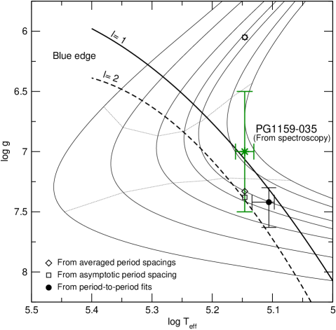
Figure 1: Our PG1159 full evolutionary tracks in the $\log T_{\rm eff}-\log g$ plane, with stellar mass (from right to left): $0.530,0.542,0.565,0.589,0.609,0.664$, and $0.742M_{\odot}$. The location of PG 1159$-$035  according to spectroscopy is indicated with a star symbol. The hollow squares (diamonds) display the predictions of the asymptotic (computed) period spacings (§3.1 and§3.2). The filled circle shows the location of PG 1159$-$035  according to the period fitting procedure (§4). Thin dotted lines define three different regimes for the theoretical rate of period change: models exhibit positive (negative) rates of period change below (above) the lower (upper) line, and positive and negative rates (between both lines). The hot boundaries of the theoretical dipole ($\ell=1$, solid line) and quadrupole ($\ell=2$, dashed line) GW Vir instability domain —according to Córsico et al. (2006)— are also shown. For details, see text.

PG 1159$-$035 is characterized by $T_{\rm eff}=140\,000\pm 5\,000$ K and $\log g=7.0\pm 0.5$ (Werner et al. 1991). Since the discovery of its photometric variations by McGraw et al. (1979), the star has been the focus of intensive scrutiny. In an impressive pulsational study, Winget et al. (1991) (WEA91) identified 122 peaks in the periodogram (Fourier spectrum) of PG 1159$-$035  obtained with the Whole Earth Telescope (WET; Nather et al. 1990). The peaks were attributed to high order nonradial $g$-modes with periods between $\approx 300-1000$ s, and with period spacings of $\Delta\Pi_{\ell=1}^{\rm O}=21.50\pm 0.03$ s and $\Delta\Pi_{\ell=2}^{\rm O}=12.67\pm 0.03$ s. The mode with the largest amplitude (7.2 mma), which was identified as a $\ell=1$, $m=+1$, has a period of $\approx 516$ s. By using a larger data set from different years (1983, 1985, 1989, 1993, and 2002) and improved data reduction and data analysis, Costa et al. (2007) (CEA07) identified 76 additional pulsation modes, enlarging to 198 the total number of pulsation periods for PG 1159$-$035, and placing it as the star with the largest number of modes detected after the Sun. CEA07 found $\Delta\Pi_{\ell=1}^{\rm O}=21.43\pm 0.03$ s and $\Delta\Pi_{\ell=2}^{\rm O}=12.38\pm 0.01$ s.

The determination of the stellar mass of PG 1159$-$035 has been the subject of numerous investigations. The stellar mass of pulsating pre-white dwarfs can be constrained from asteroseismology —the asteroseismological mass— either through the observed period spacing (see, for instance, Kawaler & Bradley 1994 (KB94); Córsico & Althaus 2006) or by means of the individual observed periods (see, e.g., KB94, Córsico & Althaus 2006, Córsico et al. 2007ac). The study of WEA91 found a mass of $0.586\pm 0.003M_{\odot}$ for PG 1159$-$035 on the basis of the observed period spacing for $\ell=1$ and $\ell=2$ modes and an asymptotic analysis based on the PG1159 structure models of Kawaler (1986, 1987, 1988). From a detailed period fit, KB94 found $M_{*}=0.59\pm 0.01M_{\odot}$ for PG 1159$-$035. Córsico & Althaus (2006) found a stellar mass of $0.56M_{\odot}$ from a period fitting procedure based on PG 1159 evolutionary models with several masses created artificially from the full sequence of $0.589M_{\odot}$ of Althaus et al. (2005). Finally, with the enlarged set of periods for PG 1159$-$035, CEA07 obtain a value of $M_{*}=0.59\pm 0.02M_{\odot}$ by using the parameterization of the asymptotic period spacing of KB94.

The total mass of PG1159 stars can also be estimated through the comparison of the spectroscopic values of $T_{\rm eff}$ and $g$ with evolutionary tracks —the spectroscopic mass. On the basis of the evolutionary tracks of O’Brien & Kawaler (2000), Dreizler & Heber (1998) derived a stellar mass of $0.54\pm 0.1M_{\odot}$ for PG 1159$-$035. The most recent determination is that of Miller Bertolami & Althaus (2006), who also derived a stellar mass of $0.54\pm 0.1M_{\odot}$ on the basis of PG1159 evolutionary models with different stellar masses that take fully into account the evolutionary history of their progenitor stars, particularly the thermally pulsing and born again phases.

The discrepancy between the asteroseismological and the spectroscopic mass of PG 1159$-$035 has been partially alleviated by the employment of Miller Bertolami & Althaus (2006) PG1159 evolutionary models and the average of the computed period spacings in the determination of the asteroseismological mass. In fact, at the effective temperature of PG 1159$-$035, the average of the computed $\ell=1$ period spacings is consistent with a stellar mass of $\approx 0.558M_{\odot}$ (Córsico et al. 2006).

The aim of this paper is to present a detailed asteroseismological study of PG 1159$-$035 based on the evolutionary models of Miller Bertolami & Althaus (2006) and the observational data of CEA07. The present study is the third time that such consistent PG1159 evolutionary models are employed in individual asteroseismological modeling of pulsating PG1159 stars, the first application being the study carried out by Córsico et al. (2007a) for the hottest known GW Vir star RX J2117.1+3412, and the second being the study performed by Córsico et al. (2007c) for the coolest member of the class, PG 0122+200.

The paper is organized as follows: in the next Section we briefly describe our PG1159 evolutionary models. In Sect. 3 we derive the stellar mass of PG 1159$-$035 by means of the observed period spacing. In Sect. 4 we derive structural parameters of this star by employing the individual observed periods. In this section we derive an asteroseismological model representative of PG 1159$-$035 (§4.3), and discuss aspects such as the mode-trapping properties (§4.4) and the rates of period changes (§4.5) of the best-fit model, and the asteroseismological distance of PG 1159$-$035 (§4.6). Finally, in Sect. 5 we summarize our main results and make some concluding remarks.

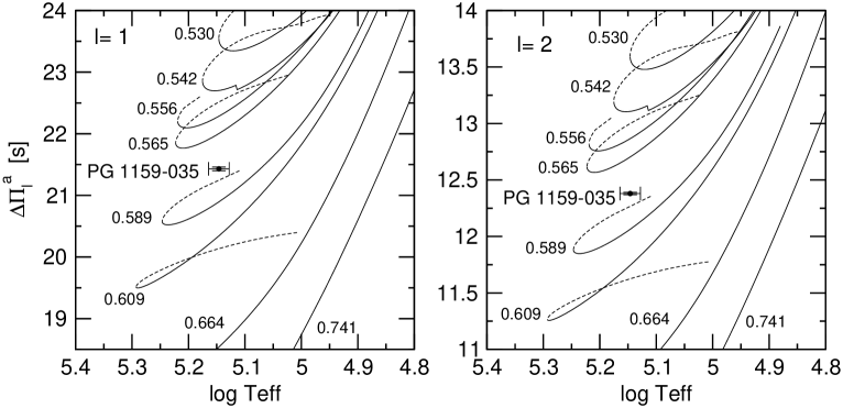
Figure 2: The dipole (left) and quadrupole (right) asymptotic period spacing ($\Delta\Pi^{\rm a}_{\ell}$) for different stellar masses in terms of the effective temperature. The stages before (after) the evolutionary “knee” are depicted with dashed (solid) lines. Numbers along each curve denote the stellar masses (in solar units). The plot also shows the location of PG 1159$-$035 according to CEA07.

2 Evolutionary models and numerical tools

The pulsation analysis presented in this work relies on a new generation of stellar models that take into account the complete evolution of PG1159 progenitor stars. Specifically, the stellar models were extracted from the evolutionary calculations recently presented by Althaus et al. (2005), Miller Bertolami & Althaus (2006), and Córsico et al. (2006), who computed the complete evolution of model star sequences with initial masses on the ZAMS in the range $1-3.75M_{\odot}$. All of the post-AGB evolutionary sequences computed with the LPCODE evolutionary code (Althaus et al. 2005) have been followed through the very late thermal pulse (VLTP) and the resulting born-again episode that give rise to the H-deficient, He-, C- and O-rich composition characteristic of PG1159 stars. The masses of the resulting remnants are 0.530, 0.542, 0.556, 0.565, 0.589, 0.609, 0.664, and $0.741M_{\odot}$. The evolutionary tracks in the $\log T_{\rm eff}-\log g$ plane for the PG1159 regime are displayed in Fig. 1.

The use of these evolutionary tracks constitutes an improvement with respect to previous asteroseismological studies. These evolutionary sequences reproduce (1) the spread in surface chemical composition observed in PG1159 stars, (2) the short born-again times of V4334 Sgr (Miller Bertolami et al. 2006 and Miller Betolami & Althaus 2007a), (3) the location of the GW Vir instability strip in the $\log T_{\rm eff}-\log g$ plane (Córsico et al. 2006), (4) the expansion age of the planetary nebula of RX J2117.1+3412 (Córsico et al. 2007ab), and (5) the period spectrum of the coolest GW Vir star, PG 0122+200 (Córsico et al. 2007c).

We computed $\ell=1$ and $\ell=2$ $g$-mode adiabatic pulsation periods with the same numerical code and methods we employed in our previous works (see Córsico & Althaus 2006 for details). We analyzed about 3000 PG1159 models covering a wide range of effective temperatures ($5.4\gtrsim\log(T_{\rm eff})\gtrsim 4.8$) and luminosities ($0\lesssim\log(L_{*}/L_{\odot})\lesssim 4.2$), and a range of stellar masses ($0.530\leq M_{*}/M_{\odot}\leq 0.741$).

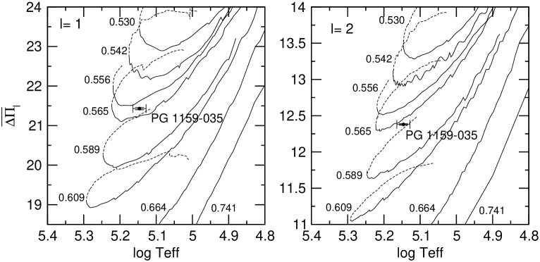
Figure 3: Same as Fig. 2, but for the average of the computed period spacings ($\overline{\Delta\Pi_{\ell}}$).

3 Mass determination from the observed period spacing

In this section we constrain the stellar mass of PG 1159$-$035 by comparing the asymptotic period spacing and the average of the computed period spacings with the observed period spacing (§3.1 and 3.2, respectively). These methods take full advantage of the fact that the period spacing of PG1159 pulsators depends primarily on the stellar mass, and weakly on the luminosity and the He-rich envelope mass fraction (KB94; Córsico & Althaus 2006).

Most of the published asteroseismological studies on PG1159 stars rely on the asymptotic period spacing to infer the total mass of GW Vir pulsators, the notable exception being the works by KB94 for PG 1159$-$035, Córsico et al. (2007a) for RX J2117.1+3412  and Córsico et al. (2007c) for PG 0122+200.

The precise evolutionary status of PG 1159$-$035 is not known a priori. Thus, we assume two possible cases in our following analysis: one situation in which the star is still on the rapid contraction phase before reaching its maximum effective temperature (i.e. before the evolutionary “knee”) and the other situation in which the star has just settled onto the white dwarf cooling track (i.e. after the evolutionary “knee”).

3.1 First method: comparison with the asymptotic period spacing, $\Delta\Pi_{\ell}^{\rm a}$

Fig. 2 displays the asymptotic period spacing for $\ell=1$ (left) and $\ell=2$ (right) modes as a function of the effective temperature for different stellar masses. Also shown in these diagrams is the location of PG 1159$-$035, with $T_{\rm eff}=140\pm 5$ kK (Werner et al. 1991), and $\Delta\Pi^{\rm O}_{\ell=1}=21.43\pm 0.03$ s and $\Delta\Pi^{\rm O}_{\ell=2}=12.38\pm 0.01$ s (CEA07). The asymptotic period spacing is computed as $\Delta\Pi_{\ell}^{\rm a}=\Pi_{0}/\sqrt{\ell(\ell+1)}$, where $\Pi_{0}=2\pi^{2}[\int_{r_{1}}^{r_{2}}(N/r)dr]^{-1}$, and $N$ the Brunt-Väisälä frequency (e.g. Tassoul et al. 1990).

From the comparison between the observed $\Delta\Pi^{\rm O}_{\ell}$ and $\Delta\Pi_{\ell}^{\rm a}$ we found a stellar mass between $\approx 0.585M_{\odot}$ (if the star is located before the evolutionary knee) and $\approx 0.577M_{\odot}$ (if the star is located after the evolutionary knee), irrespective of the $\ell$ value; see Table 1. The inferred range of mass is in agreement with the value $M_{*}\approx 0.59M_{\odot}$ derived by WEA91 and KB94 — and also in agreement with the value derived in CEA07 from the KB94 parameterization — on the basis of an asymptotic analysis of the period spacing.

As in our previous works, we must emphasize that the derivation of the stellar mass using the asymptotic period spacing may not be entirely reliable in pulsating PG1159 stars (see Althaus et al. 2007). This is because the asymptotic predictions are strictly valid in the limit of very high radial order (long periods) and for chemically homogeneous stellar models, while PG1159 stars are supposed to be chemically stratified and characterized by strong chemical gradients built up during the progenitor star life. A more realistic approach to infer the stellar mass of PG1159 stars is to compare the average of the computed period spacings with the observed period spacing.

Table 1: Stellar mass (in $M_{\odot}$) of PG 1159$-$035 derived from the period-spacing data.

	From	$\Delta\Pi^{\rm a}_{\ell}$	From	$\overline{\Delta\Pi_{\ell}}$
	$\ell=1$	$\ell=2$	$\ell=1$	$\ell=2$
Before knee	0.585	0.585	0.586	0.587
After knee	0.577	0.577	0.561	0.569

3.2 Second method: comparison with the average of the computed period spacings, $\overline{\Delta\Pi_{\ell}}$

The quantity $\overline{\Delta\Pi_{\ell}}$ is assessed by averaging the computed forward period spacings ($\Delta\Pi_{k}=\Pi_{k+1}-\Pi_{k}$) in the range of the observed periods in PG 1159$-$035: $390-990$ s for $\ell=1$ and $350-860$ s for $\ell=2$ (see Tables 4 and 12 of CEA07).

In Fig. 3 we show the run of average of the computed period spacings for $\ell=1$ (left) and for $\ell=2$ (right) in terms of the effective temperature for all of our PG1159 evolutionary sequences. Note that the run of $\overline{\Delta\Pi_{\ell}}$ depends on the range of periods on which the average of the computed period spacing is done. Again, the stages before (after) the evolutionary knee are depicted with dashed (solid) lines. By adopting the effective temperature of PG 1159$-$035  as given by spectroscopy ($T_{\rm eff}=140\pm 5$ kK) we found a stellar mass in the range $\approx 0.586-0.587M_{\odot}$ (if the star is located before the evolutionary knee) and $\approx 0.56-0.57M_{\odot}$ (if the star is located after the evolutionary knee); see Table 1. Note that these values are somewhat different to the mass derived in Córsico et al. (2006) ($\approx 0.558M_{\odot}$) because in that paper the authors used a different range of periods to compute the average of the period spacing, and a older value for observed period spacing value.

From Table 1 we see that, if the star is evolving before the knee, the value of $M_{*}$ derived from the $\overline{\Delta\Pi_{\ell}}$ is only slightly larger ($0.25\%$) than the value inferred from $\Delta\Pi_{\ell}^{\rm a}$. If star is evolving after the knee, instead, the stellar mass derived from $\overline{\Delta\Pi_{\ell}}$ is $\sim 3\%$ lower than the mass derived from $\Delta\Pi_{\ell}^{\rm a}$.

In the plot of Fig. 1, the squares correspond to the approximate location of the star as predicted by $\Delta\Pi^{\rm a}_{\ell}$, whereas the diamonds depict the situation as predicted by $\overline{\Delta\Pi_{\ell}}$. For the case in which the star is evolving before the knee, the location derived from $\Delta\Pi^{\rm a}_{\ell}$ coincides with that predicted from $\overline{\Delta\Pi_{\ell}}$. In this case the star would be located well inside the theoretical GW Vir instability strip, but the surface gravity would be excessively low ($\log g\approx 6$) as compared with the spectroscopically inferred value ($\log g=7\pm 0.5$). Thus, we will discard this solution. On the other hand, if the star is evolving after the knee, the surface gravity would be somewhat larger ($\log g\approx 7.5$) but well within the spectroscopic uncertainty, although in this case the nonadiabatic model is pulsationally stable against $\ell=1$ modes, contradicting the observational evidence.

4 Constraints from the individual observed periods

In this approach we seek a pulsation model that best matches the individual pulsation periods of PG 1159$-$035. The goodness of the match between the theoretical pulsation periods ($\Pi_{k}$) and the observed individual periods ($\Pi_{i}^{\rm O}$) is measured by means of a merit function defined as

$$\chi^{2}(M_{*},T_{\rm eff})=\frac{1}{n}\sum_{i=1}^{n}\min[(\Pi_{i}^{\rm O}-\Pi_{k})^{2}],$$ (1)

where $n$ is the total number of the observed periods considered. Note that taking the square root of $\chi^{2}$ we obtain the standard deviation between the observed and the theoretical periods. The PG 1159 model that shows the lowest value of $\chi^{2}$ will be adopted as the “best-fit model”. This approach —which is usually called the forward method in asteroseismology— has also been used in the context of pulsating PG1159 stars by Córsico & Althaus (2006) and Córsico et al. (2007ac). We evaluate the function $\chi^{2}(M_{*},T_{\rm eff})$ for stellar masses of $0.530,0.542,0.556,0.565,0.589,0.609,0.664$, and $0.741M_{\odot}$. For the effective temperature we employed a finer grid ($\Delta T_{\rm eff}\sim 100-1000$ K) which is given by the time step adopted in our evolutionary calculations.

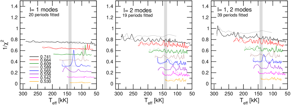
Figure 4: The inverse of the quality function corresponding to period fits considering $\ell=1$ modes only (left panel), $\ell=2$ modes only (centre panel), and $\ell=1,2$ modes simultaneously (right panel). Lines with different colours correspond to sequences with different stellar masses. Dotted (solid) lines correspond to stages before (after) the maximum effective temperature of each evolutionary sequence is reached. All of the observed $m=0$ periods were extracted from Table 3 of WEA91. For clarity, the curves have been artificially shifted upward (with a step of 0.1), except for the lower-most curve which corresponds to the $0.530M_{\odot}$ sequence. The vertical grey band displays the PG 1159$-$035  spectroscopic effective temperature and its uncertainties. [Color figure only available in the electronic version of the article]

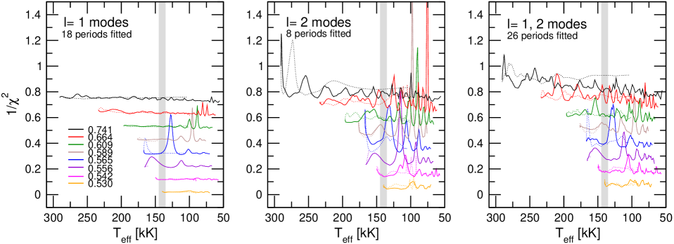
Figure 5: Same as Fig. 4, but for the case of the observed $m=0$ periods with identification secure only, extracted from Table 3 of WEA91. [Color figure only available in the electronic version of the article]

4.1 The WEA91 observed periods

Table 2: Observed periods ($\Pi_{i}^{\rm O}$) of identified $m=0$ and $\ell=1,2$ modes for PG 1159$-$035.

WEA91		CEA07		WEA91		CEA07
$\ell=1$		$\ell=1$		$\ell=2$		$\ell=2$
		390.30	s	339.24	s
		412.01	s	351.01	s	350.75
430.04	s	432.37		361.76	s	363.39
450.71		452.06	s			376.03
469.57	s	472.08		388.07	s	387.47
494.85	s	494.85	s	398.89		400.06	s
517.18	s	517.16	s	413.30	s	413.14
538.16	s	538.14	s	425.03	s	425.04
558.44	s	558.14	s	438.00	s	(437.91)
581.29		579.12		(453.62)		449.43
603.04	s	603.04				498.73	s
622.60	s	622.00				511.98	s
643.41	s	643.31	s			524.03
666.22	s	668.09				536.37
687.71	s	687.74	s			547.00
707.92	s	709.05				561.99	s
729.50	s	729.51	s	577.17	s	573.69	s
753.12	s	752.94				585.26
773.77	s	773.74		635.92
790.94	s	791.80		649.67
817.12	s	814.58				660.46
840.02	s	838.62	s			672.20
		861.72				684.48
		883.67		694.88		696.83
		903.19	s			709.87
		925.31	s	(734.87)		746.38	s
		945.01		779.48		783.19
		966.98	s	812.57		820.90	s
		988.13		833.31
						858.84
				(929.38)
				982.22
20	18	29	14	19	8	26	7

Note: parenthesis indicate $m=0$ periods which are actually absent from the power spectrum. Their values are estimated by averaging the components $m=\pm 1$.

We first performed period-to-period fits by considering the old set of PG 1159$-$035 observed $m=0$ periods of WEA91. They are reproduced in the first and third columns of our Table 2 in units of seconds. A letter “s” indicates a mode with a secure identification of $m$ and $\ell$. The last row shows the total number of periods of the corresponding column. The results of our period fits are displayed in Figs. 4 and 5, where the quantity $(\chi^{2})^{-1}$ in terms of $T_{\rm eff}$ for different stellar masses is shown. In the interest of clarity, the curves are shifted upwards with a step of 0.1 starting from the curve corresponding to the $0.530M_{\odot}$ sequence. The spectroscopic $T_{\rm eff}$ and its uncertainties are depicted with a vertical grey strip. A peak in the inverse of the merit function with $(\chi^{2})^{-1}\gtrsim 0.3$ will be considered as a good match between the theoretical and the observed periods.

We started our analysis by performing a period fit considering the supposed $m=0,\ \ell=1$ modes only (first column of Table 2). In this way, the value of $\ell$ of the computed periods is fixed to be $\ell=1$ in our period fit procedure. The function $(\chi^{2})^{-1}$ is characterized by a rather smooth behaviour except for a few pronounced peaks at stages after the turning point in $T_{\rm eff}$ is reached (left panel of Fig. 4). In particular, there exists a primary peak that is seen for the first time at high effective temperatures ($\approx 160\,000$ K) for the $0.556M_{\odot}$ sequence. The peak gradually shifts to lower $T_{\rm eff}$ for the sequences with higher masses, lying at $\sim 65\,000$ K for $M_{*}=0.741M_{\odot}$. The maximum amplitude of the peak (i.e., the best period match) is reached for a $0.565M_{\odot}$ model with $T_{\rm eff}\sim 128\,000$ K, somewhat lower than the spectroscopic effective temperature of PG 1159$-$035 ($T_{\rm eff}=140\,000\pm 5\,000$ K). In other words, if the $\ell=1$ modes were the only modes present in PG 1159$-$035, our best asteroseismological solution derived from a period fit should be a model with $T_{\rm eff}=127\,680$ K and $M_{*}=0.565M_{\odot}$. The quality of our period fit is measured by the average of the absolute period differences, $\overline{\delta\Pi_{i}}=(\sum_{i=1}^{n}|\delta\Pi_{i}|)/n$, where $\delta\Pi_{i}=\Pi_{i}^{\rm O}-\Pi_{k}$, and by the root-mean-square residual, $\sigma_{{}_{\delta\Pi_{i}}}=\sqrt{(\sum|\delta\Pi_{i}|^{2})/n}$. For this solution we obtain $\overline{\delta\Pi_{i}}=1.32$ s and $\sigma_{{}_{\delta\Pi_{i}}}=1.80$ s.

Next, we carried out a period fit taking into account the supposed $m=0,\ \ell=2$ modes only (third column of Table 2). The value of $\ell$ of the theoretical periods is fixed to be $\ell=2$. The results are depicted in the centre panel of Fig. 4. The behaviour of $(\chi^{2})^{-1}$ is very different as compared with the $\ell=1$ period fit. Remarkably, $(\chi^{2})^{-1}$ exhibits numerous peaks of almost similar amplitude, irrespective of the stellar mass. This means that the quadrupole period spectrum of the star could not be fitted by a unique PG1159 model, due to the existence of numerous and almost equivalent possible solutions . We conclude that if the $\ell=2$ modes were the only present in PG 1159$-$035, a satisfactory asteroseismological solution could not be found.

Finally we made a period fit using the $m=0,\ \ell=1$ and $m=0,\ \ell=2$ modes simultaneously (first and third columns of Table 2). In this case the value of $\ell$ for the theoretical periods is not fixed but instead is obtained as an output of our period fit procedure, although the allowed values are 1 and 2. The results are displayed in the right panel of Fig. 4. The $(\chi^{2})^{-1}$ function shows the same behaviour as in the case of the $\ell=2$ period fit. Thus, we are unable to find an asteroseismological model satisfying simultaneously both the $\ell=1$ and $\ell=2$ sets of observed periods.

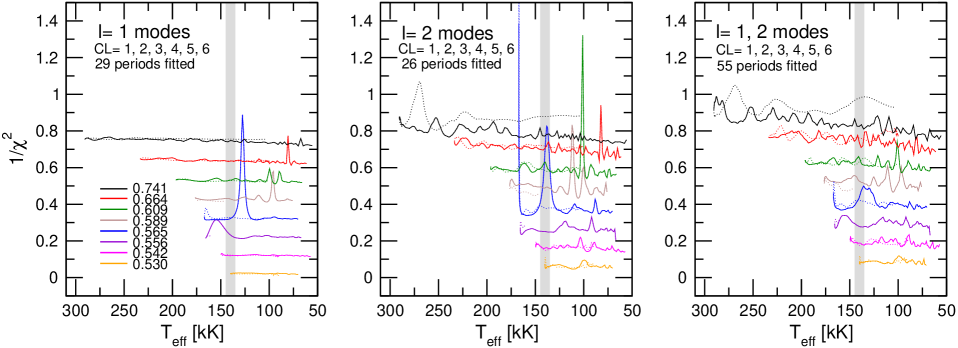
Figure 6: Same as Fig. 4. Here, all of the observed $m=0$ periods (having a Confidence Level of 1, 2, 3, 4, 5, or 6) have been extracted from Tables 4 and 12 of CEA07. [Color figure only available in the electronic version of the article]

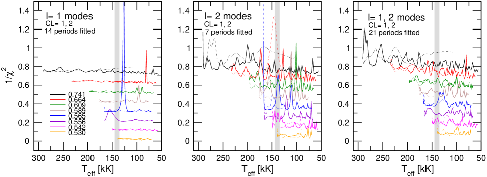
Figure 7: Same as Fig. 6, but for the case of the observed $m=0$ periods with Confidence Level of 1 or 2 only, extracted from Tables 4 and 12 of CEA07. [Color figure only available in the electronic version of the article]

Our next step was to repeat the above period fits, but this time by considering only the subset of observed periods for which the $\ell$ and $m$ identification is considered as secure and free of ambiguities by WEA91. The periods employed are labelled with a letter “s” in Table 2. As a result of this selection, the number of observed $\ell=1$ periods is slightly reduced from 20 to 18, but for $\ell=2$ modes the number is substantially reduced from 19 to 8 periods.

The results of the period fits are shown in Fig. 5. To begin with, for $\ell=1$ modes (left panel) the behaviour of $(\chi^{2})^{-1}$ remains unaltered as compared with the situation analyzed in the left panel of Fig. 4, due to both period fits being essentially the same. For the best-fit model, which is again the $0.565M_{\odot}$ model at $T_{\rm eff}=127\,680$ K, we obtain $\overline{\delta\Pi_{i}}=1.24$ s and $\sigma_{{}_{\delta\Pi_{i}}}=1.76$ s. For the $\ell=2$ period fit, on the other hand, the $(\chi^{2})^{-1}$ function experiences appreciable changes as compared with the situation analyzed before. In particular, the numerous peaks present in $(\chi^{2})^{-1}$ exhibit larger amplitudes, revealing period matches that are somewhat better as a result of the smaller number of periods to be fitted.

Finally, the simultaneous fit to $\ell=1$ and $\ell=2$ observed periods results again in a $(\chi^{2})^{-1}$ function with a complex peaked structure. Nevertheless, it is possible to distinguish in this case a prominent peak corresponding to the same best-fit model previously found, with $T_{\rm eff}=127\,680$ K and $M_{*}=0.565M_{\odot}$, and the period fit in this case is characterized by $\overline{\delta\Pi_{i}}=1.25$ s and $\sigma_{{}_{\delta\Pi_{i}}}=1.6$ s. A detailed comparison of the observed periods with the theoretical periods for this period fit is provided in Table 3.

Note that the assignation of the $\ell$ value for the theoretical periods differs from the identification of the observed periods in some cases.

4.2 The CEA07 observed periods

Table 3: Comparison between the observed $(\ell,m)=(1,0)$ and $(\ell,m)=(2,0)$ periods ($\Pi_{i}^{\rm O}$, in units of seconds) for PG 1159$-$035 taken from WEA91 and the theoretical $(\ell,m)=(1,0)$ and $(\ell,m)=(2,0)$ periods ($\Pi_{k}$, in units of seconds) of the best-fit model with $M_{*}=0.565M_{\odot}$ and $T_{\rm eff}=127\,680$ K. $\delta\Pi_{i}=\Pi_{i}^{\rm O}-\Pi_{k}$ represents the period differences, $k$ the radial orders, and $\dot{\Pi}_{k}$ the rates of period change (in units of $10^{-11}$ s/s).

$\Pi_{i}^{\rm O}$	$\ell^{\rm O}$	$\Pi_{k}$	$\ell$	$\delta\Pi_{i}$	$k$	$\dot{\Pi}_{k}$
339.24	2	340.79	2	$-1.55$	25	0.88
351.01	2	353.43	2	$-2.42$	26	0.45
361.76	2	365.04	2	$-3.28$	27	0.85
388.07	2	389.14	1	$-1.70$	16	1.22
413.30	2	412.06	1	$1.24$	17	0.75
425.03	2	426.63	2	$-1.60$	32	0.67
430.04	1	431.47	1	$-1.43$	18	0.54
438.00	2	439.28	2	$-1.28$	33	0.97
469.57	1	465.22	2	$4.35$	35	1.05
494.85	1	494.45	1	$0.40$	21	0.70
517.18	1	516.41	1	$0.77$	22	1.40
538.16	1	538.34	1	$-0.18$	23	1.05
558.44	1	558.04	1	$0.40$	24	0.77
577.17	2	576.23	2	$0.94$	44	1.72
603.04	1	602.64	1	$0.40$	26	1.03
622.60	1	621.89	1	$0.71$	27	0.98
643.41	1	644.05	1	$-0.64$	28	1.77
666.22	1	665.84	1	$0.38$	29	0.93
687.71	1	686.62	1	$1.09$	30	1.43
707.92	1	708.30	1	$-0.38$	31	1.70
729.50	1	729.32	1	$0.18$	32	1.48
753.12	1	754.38	2	$-1.26$	58	1.50
773.77	1	772.65	1	$1.12$	34	1.89
790.94	1	792.85	2	$-1.91$	61	2.38
817.12	1	816.94	2	$0.18$	63	1.73
840.02	1	837.38	1	$2.64$	37	2.38

Table 4: Observed $(\ell,m)=(1,0)$ periods ($\Pi_{i}^{\rm O}$, in units of seconds) and amplitudes (in units of mma) for PG 1159$-$035 taken from CEA07, theoretical $(\ell,m)=(1,0)$ periods ($\Pi_{k}$ in units of seconds) of the best-fit model with $M_{*}=0.565M_{\odot}$ and $T_{\rm eff}=127\,680$ K. $\delta\Pi_{i}=\Pi_{i}^{\rm O}-\Pi_{k}$ represents the period differences, $k$ are the radial orders, $\dot{\Pi}_{k}$ are the rates of period change (in units of $10^{-11}$ s/s), and $\ddot{\Pi}_{k}$ are the second order rates of period change (in units of $10^{-23}$ s/s²).

$\Pi_{i}^{\rm O}$	$A_{i}^{\rm O}$	$\Pi_{k}$	$\delta\Pi_{i}$	$k$	$\dot{\Pi}_{k}$	$\ddot{\Pi}_{k}$
390.30 s	1.0	389.14	$1.16$	16	1.22	$-0.41$
412.01 s	0.6	412.06	$-0.05$	17	0.76	$-2.54$
432.37	0.5	431.47	$0.90$	18	0.54	$1.54$
452.06 s	3.0	453.34	$-1.28$	19	1.21	$-0.26$
472.08	0.4	474.47	$-2.39$	20	0.71	$-2.30$
494.85 s	0.7	494.45	$0.40$	21	0.70	$2.08$
517.16 s	4.2	516.41	$0.75$	22	1.40	$0.14$
538.14 s	0.6	538.34	$-0.20$	23	1.05	$-2.53$
558.14 s	2.4	558.04	$0.10$	24	0.77	$1.51$
579.12	0.1	579.83	$-0.71$	25	1.65	$-0.02$
603.04	0.2	602.64	$0.40$	26	1.03	$-3.25$
622.00	0.3	621.89	$0.11$	27	0.98	$2.42$
643.31 s	0.5	644.05	$-0.74$	28	1.77	$-0.98$
668.09	0.3	665.84	$2.25$	29	0.93	$-2.65$
687.74 s	0.4	686.62	$1.12$	30	1.43	$2.65$
709.05	0.3	708.30	$0.75$	31	1.70	$-0.76$
729.51 s	0.3	729.32	$0.19$	32	1.48	$-2.81$
752.94	0.9	751.52	$1.42$	33	1.40	$1.04$
773.74	0.3	772.65	$1.09$	34	1.89	$1.92$
791.80	6.0	794.58	$-2.78$	35	2.06	$-3.98$
814.58	0.4	815.61	$-1.03$	36	1.07	$-1.37$
838.62 s	0.6	837.38	$1.24$	37	2.38	$4.41$
861.72	0.5	860.89	$0.83$	38	2.20	$-4.61$
883.67	6.0	880.45	$3.22$	39	1.42	$-2.15$
903.19 s	0.7	902.38	$0.81$	40	2.31	$2.21$
925.31 s	0.3	925.30	$0.01$	41	2.31	$-0.91$
945.01	0.3	947.13	$-2.12$	42	2.21	$-3.40$
966.98 s	0.9	967.94	$-0.96$	43	1.76	$-0.75$
988.13	0.2	989.13	$-1.00$	44	2.66	$3.69$

In this section we repeat the above analysis but this time taking full advantage of the updated and augmented set of observed periods of PG 1159$-$035 reported by CEA07. Indeed, these authors have identified 76 new pulsation modes, increasing to 198 the total number of pulsation periods of PG 1159$-$035. We reproduce in the second and fourth columns of Table 2 the subset of $\ell=1,m=0$ and $\ell=2,m=0$ periods we use here in our period fits. They correspond to Tables 4 and 12 of CEA07. In our Table 2, a letter “s” means a Confidence Level of 1 or 2. The observational uncertainties in the values of the periods are between $\sim 0.002$ and $\sim 1$ s, with an average of $\sim 0.3$ s.

We note that the pulsation periods of PG 1159$-$035 are changing with rates up to $\sim\pm 30$ ms/yr (Costa & Kepler 2007 [CK07]). So, between 1983 and 2002, the periods could have experienced variations up to $0.6$ s. Thus, for modes present in more than one periodogram, the periods in Tables 4 and 12 of CEA07 (and also in our Table 2) are the average values. At variance with this, the periods included in Table 6 of CEA07 are the values at the epoch of the largest amplitude of each mode. Thus, these periods correspond to different annual data sets. In our period fit procedure below —and also in the analysis of the period spacing of Sect. 4.4— we shall employ the set of the average values of periods (Tables 4 and 12 of CEA07) because the use of periods from different epochs (Table 6 of CEA07) seems inappropriate.

Regarding the reliability of the detected modes, CEA07 classified the possible pulsation periods by their confidence level (CL), in six different levels of decreasing probability from 1 to 6. The six probability levels are listed in Table 2 of CEA07.

The results for the $\ell=1$ period fit are displayed in the left panel of Fig.6. As previously, a quite prominent peak in $(\chi^{2})^{-1}$ is found, corresponding to the $0.565M_{\odot}$ model at $T_{\rm eff}=127\,680$ K. Remarkably, the period match turns out be of an excellent quality, with $\overline{\delta\Pi_{i}}=1.03$ s and $\sigma_{{}_{\delta\Pi_{i}}}=1.7$ s, in spite of the large number (29) of $\ell=1$ fitted periods. The recurrent presence of this solution throughout all of our period fits is striking and indicates that this PG1159 model could constitute a meaningful asteroseismological solution for PG 1159$-$035.

The results of the period fit for $\ell=2$ (centre panel of Fig. 6) are not very different from those of the $\ell=2$ period fits previously discussed. However, in the present case there exists a very pronounced peak in $(\chi^{2})^{-1}$ corresponding to a $0.565M_{\odot}$ model at $\approx 167\,000$ K, associated with a period match characterized by $\overline{\delta\Pi_{i}}=0.60$ s and $\sigma_{{}_{\delta\Pi_{i}}}=0.33$ s. Unfortunately, since this period fit relies on the observed $\ell=2$ periods only, which generally have more uncertain identifications of $\ell$ and $m$ than dipole periods, and because this solution does not also appear for the dipole modes —for which we are confident of the $\ell$ and $m$ values— we must discard this model as a meaningful asteroseismological solution for PG 1159$-$035. Other important peak seen in $(\chi^{2})^{-1}$ is located at $T_{\rm eff}\approx 100\,000$ K for $M_{*}=0.609M_{\odot}$. In decreasing order of importance, we found other peaks at $T_{\rm eff}\approx 138\,000$ K ($M_{*}=0.565M_{\odot}$), $T_{\rm eff}\approx 112\,500$ K ($M_{*}=0.589M_{\odot}$), $T_{\rm eff}\approx 83\,500$ K ($M_{*}=0.664M_{\odot}$), and $T_{\rm eff}\approx 271\,000$ K ($M_{*}=0.741M_{\odot}$).

All of the significant peaks described above are ironed out when we consider a period fit for the $\ell=1$ and $\ell=2$ periods simultaneously, as can be seen in the right panel of the Fig. 6. Again, no clear solution emerges satisfying simultaneously both the $\ell=1$ and $\ell=2$ sets of observed periods, although there is a wide bump just below $\sim 140\,000$ K for the sequence with $M_{*}=0.565M_{\odot}$.

Next, we repeated the period fits described above, but this time by considering only the most probable modes of the data set, i.e. the modes with CL= 1 or 2. Modes with CL= 1 have large amplitudes and appear in one or more of the periodograms of CEA07, whereas modes with CL= 2 have lower amplitudes but even above the detection limit, and appear in two or more periodograms. The periods of the modes with CL= 1 or 2 according CEA07 are labelled with a letter “s” in Table 2. Note that in this case the periods to be fitted are drastically reduced in number, from 29 to 14 for $\ell=1$ and from 26 to 7 for $\ell=2$.

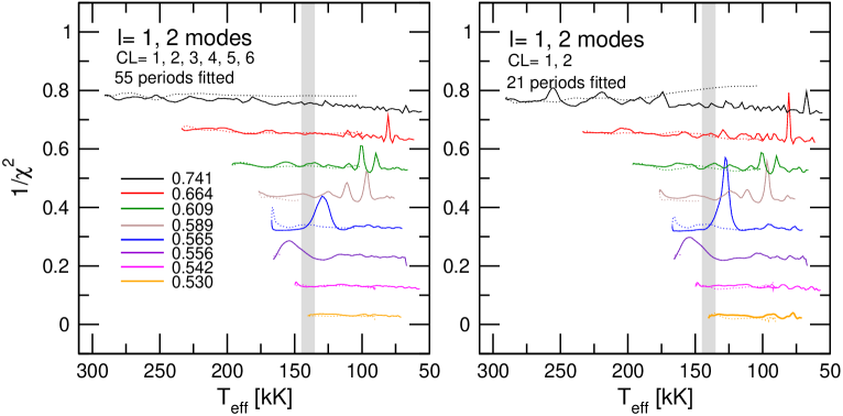
Figure 8: The inverse of the quality function corresponding to period fits considering $\ell=1,2$ modes simultaneously. Observed $\ell=1$ ($\ell=2$) periods are compared with theoretical $\ell=1$ ($\ell=2$) periods. The left panel corresponds to a period fit that includes all of the observed $m=0$ periods (having a Confidence Level of 1, 2, 3, 4, 5, or 6) extracted from Tables 4 and 12 of CEA07. The right panel corresponds to a period fit in which only the high confidence periods (those having CL= 1 or 2) are employed. [Color figure only available in the electronic version of the article]

The results of our analysis are presented in Fig. 7. Notably, for the $\ell=1$ period fit we again recover the persisting solution with $M_{*}=0.565M_{\odot}$ and $T_{\rm eff}=127\,680$ K. Remarkably, the quality of this fit for PG 1159$-$035 is much better than of those previously discussed in this paper for $\ell=1$ modes, with $\overline{\delta\Pi_{i}}=0.64$ s and $\sigma_{{}_{\delta\Pi_{i}}}=0.75$ s. A comprehensive comparison of the observed periods with the theoretical periods for this fit is provided in Table 4.

Figure 9: Same as Fig. 6, but for the case in which the observed $m=0$ periods are weighted with the square of the corresponding amplitude in the period fit procedure. [Color figure only available in the electronic version of the article]

For the $\ell=2$ period fit we obtain similar results than above (see centre panel of Fig. 7). In particular, the acute peak corresponding to the $0.565M_{\odot}$ model at $\approx 167\,000$ K persists, and in the present case it is characterized by $\overline{\delta\Pi_{i}}=0.71$ s and $\sigma_{{}_{\delta\Pi_{i}}}=0.75$ s. The new feature is the presence of a pronounced peak in $(\chi^{2})^{-1}$ corresponding to a $0.664M_{\odot}$ model at $T_{\rm eff}\sim 147\,000$ K, before the turning point in $T_{\rm eff}$ is reached. The peak at $T_{\rm eff}\approx 100\,000$ K for $M_{*}=0.609M_{\odot}$, on the other hand, has suffered from a notable reduction of its amplitude.

Again we are unable to found a unambiguous solution for the case in which the $\ell=1$ and $\ell=2$ sets of observed periods are compared simultaneously with $\ell=1,2$ theoretical periods. This is evident from the right panel of Fig. 7.

4.2.1 Fixing the $\ell$ value of the observed periods

Here we perform additional period fits for $\ell=1$ and $\ell=2$ simultaneously but forcing the $\ell=1$ observed modes to be fitted by $\ell=1$ theoretical modes, and the $\ell=2$ observed modes to be fitted by $\ell=2$ theoretical modes. In other words, we assume that the $\ell$ values adopted by CEA07 for the observed periods are correct. Fig. 8 displays in the left panel the results for a period fit considering all the periods (CL= 1, 2, 3, 4, 5, or 6) and in the right panel the results for a period fit in which only the CL= 1 or 2 are taken into account. Note that in both cases we found again the best-fit model with $M_{*}=0.565M_{\odot}$ and $T_{\rm eff}=127\,680$ K. The fact that both period fits —one involving 55 periods and the other only 21— lead to similar results lends confidence to this asteroseismological solution.

4.2.2 Weighting the period fits

We have finally performed period fits by using the observed periods of CEA07 with CL= 1, 2, 3, 4, 5 and 6, but weighting each period in the quality function $\chi^{2}$ with the corresponding amplitude. Specifically, the quality function now reads:

$$\chi^{2}(M_{*},T_{\rm eff})=\frac{\sum_{i=1}^{n}\min[(\Pi_{i}^{\rm O}-\Pi_{k})^{2}]A_{i}^{2}}{\sum_{i=1}^{n}A_{i}^{2}},$$ (2)

where we have adopted the amplitudes $A_{i}$ of the observed modes —extracted from Tables 4 and 12 of CEA07— as the weights. In this way, the period fits are more influenced by modes with large amplitudes than by modes with low amplitude. In other words, modes of large amplitude must match better the theoretical model than modes of small amplitude. Note that if we set $A_{i}=1$ for $i=1,\cdots,n$, i.e., assume the same weight for all of the modes, Eq. (2) reduces to Eq. (1), which we used in the period fits of the previous sections.

As before, in the period fits the harmonic degree was allowed to adopt the values $\ell=1$ or $\ell=2$. The results are shown in Fig. 9. Unfortunately, no apparent solution is found, neither in the case of $\ell=1$ (left panel) or $\ell=2$ (centre panel) period fits, nor in the case of period fits to $\ell=1$ and $\ell=2$ modes simultaneously (right panel). This is somehow expected since by using Eq. (2) the period fit is dominated by only a few large-amplitude modes (those with periods 390.30, 452.44, 517.16, 558.14, 791.80, and 883.67 s), whereas the remaining modes, which have notably smaller amplitudes, barely contribute to the weighting process. As a result, multiple and almost equivalent minima in the $\chi^{2}$ function are obtained, rendering it virtually impossible to find an unambiguous asteroseismological solution.

Table 5: The main characteristics of PG 1159$-$035.

Quantity	Spectroscopy	Asteroseismology	Pulsations	Asteroseismology
		(KB94)	(CEA07, CK07)	(this work)
$T_{\rm eff}$ [kK]	$140\pm 5^{\rm(a)}$	$136$	—	$128^{+8.6}_{-2.6}$
$M_{*}$ [$M_{\odot}$]	$0.54\pm 0.1^{\rm(b)}$	$0.59\pm 0.01$	$0.59\pm 0.02$	$0.565^{+0.025}_{-0.009}$
$\log g$ [cm/s2]	$7.0\pm 0.5^{\rm(a)}$	$7.38\pm 01$	—	$7.42^{+0.21}_{-0.12}$
$\log(L_{*}/L_{\odot})$	$2.73_{-0.55}^{0.41\rm(c)}$	$2.29\pm 0.05$	—	$2.15\pm 0.08$
$\log(R_{*}/R_{\odot})$	—	$-1.60\pm 0.09$	—	$-1.62^{+0.06}_{-0.09}$
$M_{\rm env}$ [$M_{\odot}$]	—	$0.002$	—	$0.017$
$r_{\rm c}/R_{*}$	—	$0.60-0.65$	$0.83\pm 0.05$	$0.55$
C/He, O/He(∗)	$1.5,0.5^{\rm(c)}$	—	—	$0.81,0.56$
$M_{\rm V}$ [mag]	—	—	—	$6.975\pm 0.4$
$M_{\rm bol}$ [mag]	—	—	—	$-0.625\pm 0.2$
$A_{\rm V}$ [mag]	—	—	—	$0.06^{+0.003}_{-0.004}$
$d$ [pc]	$800^{+600{\rm(a)}}_{-400}$	$440\pm 40$	—	$363_{-61}^{+73}$
$\pi$ [mas]	$1.25_{-0.54}^{+1.25}$	$2.27_{-0.18}^{+0.23}$	—	$2.75_{-0.46}^{+0.56}$
$\dot{R}_{*}/R_{*}$ [$10^{-11}$s-1]	—	—	$-0.89\pm 0.2$	$-0.009$
$\dot{T}/T$ [$10^{-11}$s-1]	—	—	$-1.84\pm 0.04$	$0.0004$
$k$ for $\Pi=517$ s	—	22	20	22

Note: $(*)$Abundances by mass

References: (a) Werner et al. (1991); (b) Miller Bertolami & Althaus (2006); (c) Werner & Herwig (2006).

4.3 The asteroseismological best-fit model

The results described in the last sections strongly suggest the existence of a significant asteroseismological solution for PG 1159$-$035 corresponding to a model with a stellar mass of $M_{*}=0.565M_{\odot}$ and $T_{\rm eff}=127\,680$ K. We arrive at this conclusion by considering mostly $\ell=1$ period fits, although this model also provides a good period fit for $\ell=1$ and $\ell=2$ modes simultaneously if we force observed $\ell=1$ periods to be compared with theoretical $\ell=1$ periods, and observed $\ell=2$ periods to be compared with theoretical $\ell=2$ periods (Sect. 4.2.1). Also, we found a good period fit for this model when we consider the observed periods with secure identification of WEA91, allowing the periods to be $\ell=1$ or $\ell=2$ without constraining any to be one or the other (Table 3). This model will be adopted as the “best-fit model” representative of PG 1159$-$035.

The quality of our $\ell=1$ period fits for PG 1159$-$035 using the periods of CEA07 is characterized by $\overline{\delta\Pi_{i}}=1.02$ s (when we consider modes with CL= 1, 2, 3, 4, 5, or 6; see Fig. 6) and $\overline{\delta\Pi_{i}}=0.62$ s (if we take into account modes with CL= 1 or 2 only; see Fig. 7). These period fits are of better quality than those obtained by KB94 and Córsico & Althaus (2006) ($\overline{\delta\Pi_{i}}=1.19$ s and $\overline{\delta\Pi_{i}}=1.79$ s, respectively) for PG 1159-035. The $\ell=2$ periods of our best-fit model do not match the observed quadrupole period spectrum as accurately as the dipole periods do. In spite of this fact, the best-fit model yields an average of the computed period spacings for $\ell=2$ of $\overline{\Delta\Pi_{\ell=2}}=12.61$ s, in good agreement with the observed value of $\Delta\Pi_{\ell=2}^{\rm O}=12.38\pm 0.01$ s. This property renders consistency to the derived best-fit model.

As in our previous asteroseismological analysis of GW Vir stars, we are able to get a PG1159 model that reproduces the period spectrum observed in the star under study without tuning ad hoc the value of structural parameters such as the thickness of the outer envelope, the surface chemical abundances or the shape of the core chemical profile which, instead, are kept fixed at the values predicted by the evolutionary computations.

Table 4 shows a detailed comparison between the 29 $\ell=1$ CEA07 observed periods ($\Pi_{i}^{\rm O}$) and the theoretical $\ell=1$ periods ($\Pi_{k}$) of our best-fit model. Note that if we consider all the 29 periods (CL= 1, 2, 3, 4, 5 or 6), we have $|\delta\Pi_{i}|\leq 1$ s for 17 modes ($59\%$), $1\ \mbox{s}<|\delta\Pi_{i}|\leq 2$ s for 7 modes ($24\%$), $2\ \mbox{s}<|\delta\Pi_{i}|\leq 3$ s for 4 modes ($14\%$), and $|\delta\Pi_{i}|>3$ s for 1 mode ($3.5\%$). However, if we adopt the 14 periods with the highest level of probability only (CL= 1 or 2), we obtain $|\delta\Pi_{i}|\leq 1$ s for 11 modes ($\approx 80\%$) and $1\ \mbox{s}<|\delta\Pi_{i}|\leq 2$ s for 3 modes ($\approx 20\%$).

The fifth column of Table 4 presents the radial order $k$ for the modes of our best-fit model. The $k$ values are in complete agreement with those of the best-fit model of KB94, and also in agreement (to within $\Delta k=\pm 2$) with the values proposed by CEA07. As a reference, we show the radial order of the mode with the largest amplitude ($\Pi\sim 517$ s), according to the different authors, in the last row of Table 5.

In Table 5 we show the main features of our best-fit model and also the parameters of PG 1159$-$035 extracted from other published studies. Specifically, the second column corresponds to spectroscopic results, the third column presents results from the asteroseismological analysis of KB94, the fourth column corresponds to the pulsation results of CEA07 and Costa & Kepler (2007) (CK07), and the fifth column shows the characteristics of the asteroseismological model of this work. The quoted uncertainties in the stellar mass and the effective temperature of our best fit model ($\sigma_{\rm M_{*}}$ and $\sigma_{T_{\rm eff}}$) resulting from the period fit procedure are calculated according to the following expression, derived by Zhang et al. (1986):

$$\sigma_{i}^{2}=\frac{d_{i}^{2}}{S-S_{0}}$$ (3)

where $S_{0}=\chi^{2}(M_{*}^{0},T_{\rm eff}^{0})$ is the absolute minimum of $\chi^{2}$ which is reached at ($M_{*}^{0},T_{\rm eff}^{0}$) corresponding to the best-fit model, and $S$ the value of $\chi^{2}$ when we change the parameter $i$ (in our case, $M_{*}$ or $T_{\rm eff}$) by an amount $d_{i}$ keeping fixed the other parameter. The quantity $d_{i}$ can be evaluated as the minimum step in the grid of the parameter $i$. Specifically, we use the $\ell=1$ period fit shown in the left panel of Fig. 7, that is, by considering the 14 dipole periods with CL= 1 or 2 measured by CEA07. We have $d_{T_{\rm eff}}\equiv\Delta T_{\rm eff}\sim 1000$ K and $d_{M_{*}}\equiv\Delta M_{*}$ in the range $0.009-0.024M_{\odot}$.

Our best-fit model has a stellar mass of $M_{*}=0.565M_{\odot}$, which is $\sim 1.9\%$ smaller than the value derived from the average of the computed period spacing, $M_{*}\sim 0.576M_{\odot}$, and $\sim 3\%$ lower than that inferred from the asymptotic period spacing, $M_{*}\sim 0.581M_{\odot}$ (see §3). On the other hand, CEA07 have inferred a value of the stellar mass of PG 1159$-$035 by using an interpolation formula to the period spacing derived by Kawaler & Bradley (1994) on the basis of a large grid of artificial PG1159 models in the luminosity range $1.6\lesssim\log(L_{*}/L_{\odot})\lesssim 3.0$. These authors obtain a rather high value of $0.59\pm 0.02M_{\odot}$, in line with the early determinations of WEA91 and KB94 ($0.586\pm 0.003M_{\odot}$ and $0.59\pm 0.01M_{\odot}$, respectively), but in disagreement — about $4.5\%$ larger — with the mass of our best-fit model.

Figure 10: Distribution of the forward period spacing $\Delta\Pi$ for the case of the observed periods according to Table 6 —panel (a)— and according to Table 4 —panel (b)— of CEA07.

The $M_{*}$ value of our best-fit model is somewhat higher than the spectroscopic mass of $0.54M_{\odot}$ derived by Miller Bertolami & Althaus (2006) (see also Dreizler & Heber 1998) for PG 1159$-$035. Note that a discrepancy between the asteroseismological and the spectroscopic values of $M_{*}$ is generally encountered among PG1159 pulsators (see Córsico et al. 2006, 2007ac and Althaus et al. 2007). Until now, the asteroseismological mass of PG 1159$-$035 has been about $9\%$ larger ($\Delta M_{*}\approx 0.05M_{\odot}$) than the spectroscopic mass. In light of the best-fit model derived in this paper, this discrepancy is reduced to less than about $5\%$ ($\Delta M_{*}\approx 0.025M_{\odot}$).

The location of the best-fit model in the $\log T_{\rm eff}-\log g$ diagram is displayed in Fig. 1. Note that the model is characterized by a $T_{\rm eff}$ somewhat lower than the spectroscopic value. Also, the model lies certainly slightly outside the $\ell=1$ GW Vir instability domain, at odds with the observational evidence.

4.4 Period spacing and mode trapping

The mode-trapping properties of PG1159 stars have been discussed at length by KB94 and Córsico & Althaus (2006); we refer the reader to those works for details. We will consider the observed $\ell=1$ forward period spacing ($\Delta\Pi=\Pi_{k+1}-\Pi_{k}$) taking advantage of the uninterrupted string of 29 dipole periods with consecutive radial orders from $k=14$ to $k=42$, according CEA07.

In panel (a) of Fig. 10 we show the $\Delta\Pi$ vs $\Pi$ diagram for the observed periods according to Table 6 of CEA07. The uncertainties in the observed period spacings are between $0.01$ and $1.2$ s, with an average value of $0.4$ s. As we mentioned at the beginning of Sect. 4.2, the periods of PG 1159$-$035  are changing with time. So, the values included in Table 6 of CEA07 are the periods corresponding to the epoch of the largest amplitude of each mode. This diagram is used by those authors to identify five modes trapped in the He-rich envelope of PG 1159$-$035. They arrive at this conclusion under the assumption that trapped modes appear as points of minimum in this diagram. By assuming the presence of a single chemical interface, CEA07 derive $r_{\rm c}/R_{*}\approx 0.83$, where $r_{\rm c}$ is the radial coordinate of the O/C/He chemical interface. In our best-fit model this chemical interface is located at markedly deeper layers ($r_{\rm c}/R_{*}\approx 0.55$), in agreement with the models of KB94 ($r_{\rm c}/R_{*}\approx 0.60-0.65$).

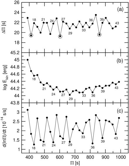
Figure 11: Panel (a): distribution of $\Delta\Pi$ for the best-fit model, the primary minima being marked with circles. Panel (b): the computed distribution of the kinetic energy. Panel (c): the theoretical values of the relative rates of period change. Modes trapped in the outer envelope model are labelled with their radial order $k$.

Note that some periods used to construct the diagram of panel (a) in Fig. 10 (extracted from Table 6 of CEA07) slightly differ from the periods included in Table 4 of CEA07 (and in our Tables 2 and 4) because, as stated before, they are the average values of periods on several annual data sets. The slight differences in some of the periods are translated into appreciable differences in some values of the period spacing, as can be seen in panel (b) of Fig. 10, where we plot the same diagram but on the basis of the periods given in Table 4 of CEA07. Since the period fits performed in the present work are based on these periods, we shall concentrate on the diagram of panel (b) of Fig. 10. It can be compared with panel (a) of Fig. 11, in which the $\Delta\Pi$ vs $\Pi$ diagram for the best-fit model is displayed. Note that, in spite of the excellent match between the observed periods and the theoretical periods of the best-fit model (Table 4), the pertinent period spacing distribution looks somewhat different. The disagreement has its origin in the fact that small differences in period —because the period match is not perfect— are translated into large differences in period spacing. Besides the disagreement between individual values of $\Delta\Pi$, we note that generally the amplitude of the observed period spacing are remarkably larger than that of the best-fit model. This suggests that the chemical interfaces present in PG 1159$-$035  could be considerably steeper than predicted by our PG1159 modeling.

Notwithstanding the mentioned differences between the period spacing distributions in PG 1159$-$035  and in our best-fit model, they share a common feature: both exhibit primary and secondary minima, characteristic of mode trapping due to the presence of more than one chemical interfaces. In fact, our best-fit model has two chemical transition regions: the inner interface of O/C and the more external interface of O/C/He. As we have already demonstrated (see, e.g., Córsico & Althaus 2006 and Córsico et el. 2007ac), for periods below $\approx 650-700$ s the mode-trapping features of our PG1159 models are induced mostly by the chemical gradient at the O/C/He interface, the O/C interface being more relevant for longer periods. We conclude that the presence of primary and secondary minima in the $\Delta\Pi_{k}$ pattern of PG 1159$-$035 is an indication that the star could be characterized by more than one chemical interfaces, possibly two.

Regarding the identification of trapped modes by means of the $\Delta\Pi$ vs $\Pi$ diagram —which constitutes the main observational tool of mode trapping in PG1159 stars— we emphasize that generally a trapped mode with radial order $k$ is associated with a minimum $\Delta\Pi$ which corresponds to a radial order $k\pm 1$, and in some cases to $k$. This is illustrated in panel (b) of Fig. 11, in which we show the kinetic energy distribution $E_{\rm kin}$, of our best-fit model. Local minima in the $E_{\rm kin}$ distribution correspond to trapped modes, because these modes propagate mainly in the low density regions of the outer He-rich envelope. Note that, for instance, the minimum of $\Delta\Pi$ with radial order $k=23$ is related to a minimum in $E_{\rm kin}$ of the trapped mode with $k=24$. Modes trapped in the envelope are also characterized by minima in $\dot{\Pi}/\Pi$, because they should be more strongly sensitive to the effects of the surface contraction —that induces a secular decrease of the periods— than untrapped modes —which are more affected by cooling. This effect is well illustrated in panel (c) of Fig. 11.

4.5 Period changes and the cooling rate of PG 1159$-$035

In Table 4 we show the rate of period change for the modes of our best-fit model (sixth column). Our calculations predict all of the pulsation periods to increase with time ($\dot{\Pi}>0$), in accordance with the decrease of the Brunt-Väisälä frequency in the core of the model induced by cooling. This property is shared by all of the PG1159 models located below the lower thin dotted line in Fig. 1. Note that at the effective temperature of our best-fit model, cooling possibly has the largest effect on $\dot{\Pi}$, but gravitational contraction —which should result in a decrease of periods with time— is not negligible and could affect the $\dot{\Pi}$ values, in particular for the case of modes trapped in the envelope (see Fig. 11).

Our best fit model does not reproduce the recent measurements of CK07, which indicate that the pulsation modes of PG 1159$-$035 have positive and negative values of $\dot{\Pi}$. Our PG1159 models having a mix of positive and negative $\dot{\Pi}$ values are located between the two thin dotted lines in Fig. 1. Remarkably, the measurements of CK07 are consistent with the spectroscopic location of PG 1159$-$035 on the $\log T_{\rm eff}-\log g$ diagram. Thus, to be consistent with the findings of CK07 our best-fit model for PG 1159$-$035 should be located at earlier evolutionary stages.

CK07 report values of the rate of period change in PG 1159$-$035  that are generally more than one order of magnitude larger than the theoretical $\dot{\Pi}$ values characterizing our best-fit model. In particular, they report $\dot{\Pi}=(+18.2\pm 0.8)\times 10^{-11}$ s/s for the large amplitude $m=0,\ \ell=1$ mode with period 517.1 s, excessively larger than the value predicted by our computations for that mode ($\dot{\Pi}=1.40\times 10^{-11}$ s/s). In addition, CK07 have been able to measure the second order rates of period change ($\ddot{\Pi}$) for eight modes in PG 1159$-$035. Again, the measured values ($|\ddot{\Pi}|\sim 0.01-9\times 10^{-19}$ ss^-2) are strikingly larger than our theoretical predictions ($|\ddot{\Pi}|\sim 0.1-5\times 10^{-23}$ ss^-2).

Finally, by using the $\dot{\Pi}/\Pi$ values measured for the ($m=0$) 517.1 s and the ($m=+1$) 516.0 s modes, CK07 roughly estimate for PG 1159$-$035 a contraction rate of $\dot{R}_{*}/R_{*}=-8.9\pm 0.2\times 10^{-12}$s^-1 and a cooling rate of $\dot{T}/T=-1.84\pm 0.04\times 10^{-11}$s^-1, orders of magnitude larger than our theoretical predictions for the best-fit model, of $\dot{R}_{*}/R_{*}=-9.0\times 10^{-14}$s^-1 and $\dot{T}/T=4.0\times 10^{-15}$s^-1.

4.6 The asteroseismological distance and parallax of PG 1159$-$035

We employ the luminosity of our best-fit model to infer the seismic distance of PG 1159$-$035 from the Earth. First, we compute the bolometric magnitude from the luminosity of the best-fit model by means of $M_{\rm bol}=M_{\odot{\rm bol}}-2.5\log(L_{*}/L_{\odot})$, with $M_{\odot{\rm bol}}=4.75$ (Allen 1973). Next, we transform the bolometric magnitude into the absolute magnitude, $M_{\rm v}=M_{\rm bol}-{\rm BC}$, where ${\rm BC}$ is the bolometric correction. For PG 1159$-$035 we adopted ${\rm BC}=-7.6\pm 0.2$ from Werner et al. (1991). We account for the interstellar absorption, $A_{\rm V}$, using the interstellar extinction model developed by Chen et al. (1998). We compute the seismic distance $d$ according to the well-known relation: $\log d=\frac{1}{5}\left[m_{\rm v}-M_{\rm v}+5-A_{\rm V}(d)\right]$ where the apparent magnitude is $m_{\rm v}=14.84$. The interstellar absorption $A_{\rm V}(d)$ varies non linearly with the distance and also depends on the Galactic latitude ($b$) and longitude ($\ell$). For the equatorial coordinates of PG 1159$-$035  (Epoch B2000.00, $\alpha=12^{\rm h}\ 1^{\rm m}\ 46^{\rm s}.1$, $\delta=-3^{\circ}\ 45^{\prime}\ 39^{\prime\prime}$) the corresponding Galactic coordinates are $b=-56^{\circ}\ 51^{\prime}\ 55^{\prime\prime}.44$ and $\ell=279^{\circ}\ 49^{\prime}\ 10^{\prime\prime}.2$. We solve for $d$ and $A_{\rm V}$ iteratively and obtain a distance $d\sim 360$ pc and an interstellar extinction $A_{\rm V}\sim 0.06$. Note that our distance is a factor of more than two smaller than the estimation of $800^{+600}_{-400}$ of Werner et al. (1991) and with its accuracy substantially improved. Finally, our calculations predict a parallax of $\pi\sim 2.8$ mas.

5 Discussion and conclusions

In this paper we carried out a comprehensive asteroseismological study of PG 1159$-$035, a $g$-mode pulsator that defines the class of pulsating PG1159 stars — the GW Vir variables— and the PG 1159 spectral class of hydrogen-deficient stars. Our analysis is based on the full PG1159 evolutionary models presented in Althaus et al. (2005), Miller Bertolami & Althaus (2006), Córsico et al. (2006) and Córsico et al. (2007c). These models represent a solid basis to analyze the evolutionary and pulsational status of GW Vir stars like PG 1159$-$035.

We first took advantage of the strong dependence of the period spacing of variable PG1159 stars on the stellar mass, and derived a value of the mass in the range $0.577-0.585M_{\odot}$ by comparing the observed mean period spacing $\Delta\Pi^{\rm O}$ with the asymptotic period spacing of our models. We also compared $\Delta\Pi^{\rm O}$ with the computed period spacing averaged over the period range observed in PG 1159$-$035, and derived a value in the range $0.561-587M_{\odot}$. Note that in both derivations of the stellar mass we made use of the spectroscopic constraint that the effective temperature of the star should be $\sim 140$ kK.

Next, we adopted a less conservative approach in which the individual observed pulsation periods alone —i.e., ignoring “external” constraints such as the spectroscopic values of the surface gravity and effective temperature— naturally lead to an “asteroseismological” PG1159 model that is assumed to be representative of the target star. Specifically, the method consists in looking for the model that best reproduces the observed periods. The period fits were made on a grid of PG1159 models with a quite fine resolution in effective temperature although admittedly coarse in stellar mass. We employed the period data from WEA91 and also the more modern — and enlarged— period data of CEA07. We considered period fits taking into account observed $\ell=1$ modes only, observed $\ell=2$ modes only, and observed $\ell=1$ and $\ell=2$ modes simultaneously. We found a persisting and significant asteroseismological solution for PG 1159$-$035 corresponding to a model with a stellar mass of $M_{*}=0.565M_{\odot}$ and $T_{\rm eff}=127\,680$ K whose $\ell=1$ periods match the observed periods identified as $\ell=1$ with an average of the period differences (observed versus theoretical) of only $0.64$ s (for 14 $\ell=1$ periods fitted) and $1.03$ s (for 29 $\ell=1$ periods fitted). Also, for this “best-fit model” we obtain a good period match when we consider a period fit for dipole and quadrupole modes simultaneously if we constrain the $\ell$ value of the input periods from the outset.

The main results of this work are summarized in Fig. 1 and Table 5, where the best-fit model solution as well as the inferences from the period spacing analysis are displayed together with the spectroscopic inferences. Note that the best-fit model is characterized by a stellar mass similar to the mass value predicted by the period spacing approach, although with a lower effective temperature (slightly outside the 1 $\sigma$ error bar). However, at this location, and according to the nonadiabatic pulsation analysis of the PG1159 sequences employed here (Córsico et al. 2006) the model should be pulsationally stable against $\ell=1$ modes and the rates of period changes all positive, in disagreement with the observations. In this sense, we must warn the reader that the location of the theoretical blue edge of the GW Vir instability strip shown in Fig. 1 is not to be taken at face value. This is because changes in the surface abundances predicted by stellar modeling are expected to shift the predicted blue edge location. For instance, Quirion et al. (2007) have found that increasing the carbon and oxygen abundance in the outer layers shifts the blue edge to larger effective temperatures. In particular, by varying the oxygen abundance from $X_{\rm O}\sim 0.20$ to $0.40$ (with He being replaced by O) and keeping fixed the carbon abundance at $X_{\rm C}\sim 0.40$, the blue edge of the GW Vir instability strip can be pushed to higher effective temperatures by about $10\,000$ K.

We can independently constrain the location of PG 1159$-$035  in the $\log T_{\rm eff}-\log g$ plane by examining the trend of secular period changes. In fact, CK07 have reported the period change of 27 pulsation modes. They found that some modes show an increase in their periods, while other exhibit a clear decrease. This could be reflecting that PG 1159$-$035 is a pre-white dwarf that still has significant ongoing contraction. To elaborate this point further, we mark in Fig. 1 with thin dotted lines the limits of the region for which our PG1159 sequences predict the simultaneous presence of modes with positive and negative $\dot{\Pi}$ . To be consistent with the findings of CK07 our best-fit model for PG 1159$-$035 should be located at earlier evolutionary stages, as suggested by spectroscopy. In fact, our predicted best-fit model falls in the region of the $\log T_{\rm eff}-\log g$ diagram where all of the pulsational modes are expected to exhibit a positive value of the period change.

Finally, we note that generally the rates of period change measured by CK07 are about one order of magnitude larger than the values predicted by the best-fit model. This is particularly true for the large amplitude mode at 517.1 s, for which CK07 report a value $\dot{\Pi}=(+18.2\pm 0.8)\times 10^{-11}$ s/s, at odds with our theoretical value $\dot{\Pi}=1.40\times 10^{-11}$ s/s — the same problem occurs with all other previous calculations, including those of Kawaler (1986). Also, our best-fit model for PG 1159$-$035 fails to reproduce the large values of the second order rates of period changes observed in the star, and the contraction and cooling rates estimated by CK07. Those authors do point out that these estimates need corroboration.

The results of the period-fit procedure carried out in this work suggest that the asteroseismological mass of PG 1159$-$035  ($\sim 0.565M_{\odot}$) could be $\sim 4\%$ lower than thought hitherto ($\sim 0.59M_{\odot}$; see WEA91, KB94 and more recently CEA07) and in closer agreement with the spectroscopic mass of $0.54M_{\odot}$ as derived by Miller Bertolami & Althaus (2006) (see also Dreizler & Heber 1998). This suggests that a reasonable consistency between the asteroseismological mass and the spectroscopic mass should be expected when the same evolutionary tracks are used for both derivations of $M_{*}$, as we have done in Córsico et al. (2007c) for PG 0122+200 and we do in the present work for PG 1159$-$035. The exception to this assertion is RX J2117.1+3412, for which we found an asteroseismological mass about $25\%$ lower than the spectroscopic value (Córsico et al. 2007ac), employing the same stellar evolution and pulsation modeling as in the present work. As we suggested in that paper, the discrepancy in mass could be due to large errors in the spectroscopic determination of $\log g$ and $T_{\rm eff}$ for RX J2117.1+3412. Uncertainties in the location of the evolutionary tracks in the HR and $\log T_{\rm eff}-\log g$ diagrams due to the modeling of PG1159 stars and their precursors can be discarded in view of the recent work by Miller Bertolami & Althaus (2007b). They conclude that the tracks of PG1159 stars of Miller Bertolami & Althaus (2006) are robust enough as to be used for spectroscopical mass determinations of PG 1159-type stars.

In closing, in this paper we have been able to find a PG1159 model that reproduces the observed pulsation periods of PG 1159$-$035 without invoking any artificial adjustments of the structural parameters (the O/C chemical profile, the surface He abundance, or the thickness of the He-rich envelope) which, instead, are kept fixed at the values predicted by our evolutionary computations. In particular, our PG1159 models are characterized by thick He-rich envelopes.

However, our best-fit model is unable to explain a number of important observed properties of PG 1159$-$035, such as:

• the nature itself of PG 1159$-$035 as a variable star, because the best-fit model lies outside the theoretical dipole GW Vir instability domain, i.e., the nonadiabatic treatment indicates pulsational stability of the model against $\ell=1$ $g$-modes,

• the larger range of the period spacings of PG 1159$-$035, as compared with those of the best-fit model,

• the mixture of positive and negative rates of period change measured in PG 1159$-$035, because the best-fit model has all the theoretical rates of period changes positive,

• the large magnitude of the rates of period change detected in PG 1159$-$035, because they are an order of magnitude larger than the theoretical values of the best-fit model.

In view of the above shortcomings, we must investigate if PG 1159$-$035 could harbor a thinner helium-rich envelope than predicted by our evolutionary models, a possibility sustained by the fact that PG 1159 and born-again stars are observed to suffer from appreciable mass loss. Further asteroseismological analysis on the basis of PG1159 evolutionary models characterized by thin He-rich envelopes, and additional observational campaigns will be needed to make definite conclusions about the internal structure and evolutionary status of PG 1159$-$035.

- (1) Althaus, L. G., Serenelli, A. M., Panei, et al. 2005, A&A, 435, 631
- (2) Althaus, L. G., Córsico A. H., Kepler, S. O. & Miller Bertolami, M. M. 2007, A&A, submitted
- (3) Blöcker, T. 2001, Ap&SS, 275, 1
- (4) Córsico, A. H., & Althaus, L. G. 2006, A&A, 454, 863
- (5) Córsico, A. H., Althaus, L. G., & Miller Bertolami, M. M. 2006, A&A, 458, 259
- (6) Córsico, A. H., Althaus, L. G., Miller Bertolami, M. M., & Werner, K. 2007a, A&A, 461, 1095
- (7) Córsico, A. H., Althaus, L. G. & Miller Bertolami, M. M. 2007b, A&A, 470, 1021
- (8) Córsico, A. H., Miller Bertolami, M. M., Althaus, L. G., Vauclair, G., & Werner, K. 2007c, A&A, in press
- (9) Costa, J. E. S., Kepler, S. O., Winget, D. E., et al. 2007, A&A, to be published (ArXiv e-prints, 711, arXiv:0711.2244) (CEA07)
- (10) Costa, J. E. S. & Kepler, S. O. 2007, A&A, submitted (CK07)
- (11) Dreizler, S., & Heber, U. 1998, A&A, 334, 618
- (12) Gautschy, A., Althaus, L. G., & Saio, H. 2005, A&A, 438, 1013
- (13) Herwig, F. 2001, ApJ, 554, L71
- (14) Kawaler, S. D., & Bradley, P. A. 1994, ApJ, 427, 415 (KB94)
- (15) Kawaler, S. D. 1986, Ph.D. Thesis, University of Texas
- (16) Kawaler, S. D. 1987, in Stellar Pulsation, Ed. A. N. Cox, W. M. Sparks, & S. G. Starrfield (Berlin: Springer), 367
- (17) Kawaler, S. D. 1988, in IAU Symposium 123, Advances in Helio- and Asteroseismology, ed. J. Christensen-Dalsgaard & S. Frandsen (Dordrecht: Reidel), 329
- (18) Lawlor, T. M., & MacDonald, J. 2003, ApJ, 583, 913
- (19) McGraw, J. T., Starrfield, S. G., Liebert, J., Green, R. F. 1979, in: White dwarfs and variable degenerate stars. (Rochester, NY) 377
- (20) Miller Bertolami, M. M., & Althaus, L. G. 2007a, MNRAS, 380, 763
- (21) Miller Bertolami, M. M., & Althaus, L. G. 2007b, A&A, 470, 675
- (22) Miller Bertolami, M. M., & Althaus, L. G. 2006, A&A, 454, 845
- (23) Miller Bertolami, M. M., Althaus, L. G., Serenelli, A. M., & Panei, J. A. 2006, A&A, 449, 313
- (24) Nather, R. E., Winget, D. E., Clemens, J. C., Hansen, C. J., Hine, B. P. 1990, ApJ, 361, 309
- (25) O’Brien, M. S., & Kawaler, S. D. 2000, ApJ, 539, 372
- (26) Quirion, P.-O., Fontaine, G., & Brassard, P. 2007, ApJS, 171, 219
- (27) Starrfield, S. G., Cox, A. N., Hodson, S. W., & Pesnell, W. D. 1983, ApJ, 268, L27
- (28) Tassoul, M., Fontaine, G., & Winget, D. E. 1990, ApJS, 72, 335
- (29) Werner, K., & Herwig, F. 2006, PASP, 118, 183
- (30) Werner, K., Heber, U., & Hunger, K. 1991, A&A, 244, 437
- (31) Winget, D. E., Nather, R. E., Clemens, J. C., et al. 1991, ApJ, 378, 326 (WEA91)
- (32) Zhang, E.-H., Robinson, E. L., & Nather, R. E. 1986, ApJ, 305, 740