Quantum Computational Method of Finding the Ground State Energy and Expectation Values
Abstract
We propose a new quantum computational way of obtaining a ground-state energy and expectation values of observables of interacting Hamiltonians. It is based on the combination of the adiabatic quantum evolution to project a ground state of a non-interacting Hamiltonian onto a ground state of an interacting Hamiltonian and the phase estimation algorithm to retrieve the ground-state energy. The expectation value of an observable for the ground state is obtained with the help of Hellmann-Feynman theorem. As an illustration of our method, we consider a displaced harmonic oscillator, a quartic anharmonic oscillator, and a potential scattering model. The results obtained by this method are in good agreement with the known results.
pacs:
03.67.Lx, 03.67.Mn, 03.65.UdI Introduction
Quantum simulation might be a real application of medium-scale quantum computers with qubits Schack06 . As Feynman suggested, a quantum computer can simulate quantum systems better than a classical computer because it is also a quantum system Feynman82 . Lloyd demonstrated that almost all quantum systems can be simulated on quantum computers Lloyd96 . Abrams and Lloyd presented a quantum algorithm to find eigenvalues and eigenvectors of a unitary operator based on the quantum phase estimation algorithm Abrams99 . Although it is an efficient quantum algorithm, there is room for improvement. First, one has to prepare an input state close to unknown eigenstates. Second, it has been little explored how to obtain physical properties except the energy spectrum.
In this paper, we propose a new refined quantum computational method to calculate the ground state energy and expectation values of observables for interacting quantum systems. The main idea is as follows. Adiabatic turning on an interaction makes the ground state of a non-interacting system evolve to the ground state of an interacting system. During the adiabatic evolution, the phase estimation algorithm extracts the phase of an evolving quantum system continuously without the collapse of a quantum state. So the ground energy of an interacting system is obtained as a function of coupling strength. With the help of the Hellmann-Feynman theorem Hellmann , the expectation value of an observable for the ground state of an interacting system is obtained. As a test of our method, we simulate on classical computers three quantum systems: a displaced harmonic oscillator, a quartic anharmonic oscillator Bender69 , and a potential scattering model Kehrein .
II Method
Let us start with a brief review of Abrams and Lloyd’s algorithm. Its goal is to find eigenvalues and eigenstates of a time-independent Schrödinger equation
| (1) |
Their key idea to solve (1) is to consider its time evolution
| (2) |
where is an input or trial state. The information on eigenvalues in the input state is transfered to index qubits by applying the quantum phase estimation algorithm. The measurement of the index qubits gives us a good approximation to with probability , and makes collapse to . It is instructive to compare (2) with the quantum Monte Carlo method which uses the imaginary time to project the input state onto the ground state Foulkes01
| (3) |
First, in order to find the ground state energy, both (2) and (3) require a good input state close to . If the input state does not contain the information about the ground state, both will fail. Second, for each run, while (2) outputs randomly, (3) produces always. Finally, (2) is a real time evolution, however, (3) is the imaginary time evolution, i.e., a diffusion process, which is implemented by classical random walks.
Our goal is to find a ground state energy with probability 1 even if an input state contains little information on the ground state. Our method uses a real time projection onto the ground state by adiabatically turning on an interaction. Ortiz et al. suggested the use of the Gell-Mann-Low theorem to find the spectrum of a Hamiltonian with quantum computers Gellmann51 ; Ortiz01 . Farhi et al. developed the adiabatic quantum computation Farhi01 .
We divide the Hamiltonian into two parts: non-interacting Hamiltonian and interaction , , As usual, it is assumed that the eigenvalues and eigenstates of are known, . We recast to be time-dependent
| (4) |
where a slowly varying function satisfies and with running time . The role of the constant energy will be explained later. As the interaction is turned on slowly, the input state evolves adiabatically to
| (5) |
where is a time-ordering operator Geomtric . Notice the similarity and difference between (2), (3), and (5). The quantum phase estimation algorithm can extract the information on from (5). Since, during the adiabatic evolution, the quantum system is in an instantaneous ground state of , one can apply frequently the phase estimation algorithm without the collapse of the quantum state to the exited states.
Since the phase is defined in , the phase estimation algorithm gives us only the absolute value of an energy . Its sign can be determined by adding . When is negative, while is positive, makes all the spectrum positive. Also is useful for stabilizing the algorithm. If is close to zero, a long time needs to make the phase finite.
The expectation value of an observable can be obtained with the help of the Hellmann-Feynman theorem Hellmann . It states that if with parameter , then the following relation holds
| (6) |
By modifying the full Hamiltonian to have a linear coupling to , , (6) becomes
| (7) |
Therefore, the expectation value of an observable is obtained from a derivative of at . In practice, (7) is obtained from a numerical approximation . This is comparable with an expectation estimation algorithm Knill07 . Notice that our scheme does not require the repeated measurements and the average over the individual outcomes Schack06 .
III Application to Quantum Systems
III.1 Displaced harmonic oscillator
As an illustration of our method, let us consider a simple Hamiltonian,
| (8) |
For convenience, we set . It is well known that (8) is exactly solvable, a usual perturbation theory for it works well, and its ground state is a coherent state.
The first step to quantum simulation is to map a physical system to a qubit system. The position in (8) is continuous, but qubits are discrete. A usual approach is to discretize . Another way is to map the eigenstates of to the computational basis of qubits, with and or . Then is given by a diagonal matrix,
| (9) |
The quantum dynamics of (9) was simulated on an NMR quantum computer by Somaroo et al. Somaroo99 . On the other hand, is written as a tridiagonal matrix,
| (10) |
A quantum state at time can be expressed in terms of , .
The adiabatic time evolution (5) is implemented by solving the time-dependent Schrödinger equation with the forth-order Runge-Kutta method on a classical computer. We take . We assume hat the phase estimation algorithm is implemented very accurately. The adiabatic switching-on function used here is given by . One may expect it would take a long time for a quantum system to evolve adiabatically. However, in the case considered here, it takes the running time to obtain the ground state energy with accuracy , where is the period of the ground state of , , and is the numerical value.
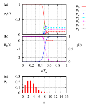
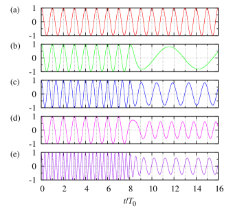
Fig. 1 shows how the dynamical phase of the system changes as the interaction is slowly turned on. In Fig. 1 (a), , and the oscillation period is . Figs. 1 (b) and (c) show how the constant energy is used to change the frequency corresponding to the ground state energy of an interacting Hamiltonian. In Fig. 1 (b), and . So the frequency become very low. However, in Fig. 1 (c), the constant energy shifts the frequency so it can be easily measured. In Figs. 1 (d) and (e), we take so the exact energy is . Since the phase estimation algorithm produces only the absolute value of energy, , the constant energy is added in (4) to decide its sign. In Fig. 1 (d), . At the end of running, the estimated energy is . So the phase estimation algorithm fails to calculate the exact ground state energy . However, in Fig. 1 (e), . the phase estimation algorithm gives us the energy . So we know that the exact energy is .
For any , the ground state of (8) is a coherent state. As shown in Fig. 2, the probability that qubits are in the number state follows a Poisson distribution. So the ground state obtained by the quantum simulation might be called a pseudo-coherent state because it is defined on the truncated Hilbert space. It is a collective state of qubits.
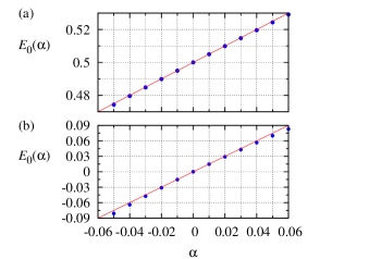
The coherent state is also characterized by the minimum uncertainties in and . Its mean square deviation of , is for any . The ground state of (8) is displaced from the origin to . So . With the help of the Hellmann-Feynman theorem, we calculate for and . To this end, the final Hamiltonian is modified as . Fig. 3 shows the ground state energy as a function of . The derivative of at gives us the expectation value of , As illustrated in Fig. 3, we have for . Thus . For , . Again we have .
III.2 Quartic anharmonic oscillator
Let us consider an anharmonic oscillator, whose Hamiltonian is given by
| (11) |
where is the coupling constant. In their seminal paper Bender69 , Bender and Wu showed that the Rayleigh-Schrödinger perturbation theory for (11) becomes divergent for any . Various non-perturbative methods have been applied to this simple model.
One can write , where
| (12) |
The matrix of (12) is more denser than (10). So more qubits are used in (12) in order to get the accurate energy.
III.3 Potential scattering model
Finally, we consider spinless electrons with a contact potential with Hamiltonian
| (13) |
where with level spacing , is a creation operator, and the coupling constant. Although this model is very simple and exactly solvable, it contains rich physics Kehrein . The naive perturbation theory breaks down no matter small is. For an attractive potential, i.e., , the lowest eigenstate of (13) becomes a bound state. Also it exhibits the Anderson orthogonality catastrophe Anderson67 which states that the ground state of becomes orthogonal to the ground state of in the thermodynamic limit.
We map the single-particle energy level of to a computational basis, , where is a vacuum state. In (13), can be written as a diagonal matrix, . Whereas are given by , which is more dense than (10) and (12).
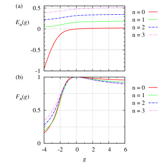
As is turned on adiabatically, the initial state evolves to the final state . We use the notation . Fig. 5 (a) illustrates the single-particle levels . One see that there is one bound state with negative energy for , but otherwise it is positive. Fig. 5 (b) shows the fidelity as a function of . Surprisingly, it is also calculated with the help of the Hellmann-Feynman theorem. One can rewrite with . As shown in Fig. 5 (b), the fidelity decrease more rapidly for than for . One can see that even single-particle levels for and become orthogonal. It is interesting that the fidelity between the interacting and non-interacting many-body ground states can be obtained from all the information of single-particle levels Ohtaka90 .
IV conclusions
In conclusion, we have proposed a new method to find the ground state energy by adiabatically turning on an interaction. The expectation values of an observable has been obtained by switching on a modified interaction which contains an observable and by applying the Hellmann-Feynman theorem. Our method has been successfully tested by solving three quantum systems. We expect that our method could be applied to the simulation of more interesting quantum systems.
Finally, let us discuss the limits of our method. Our method is based on the combination of adiabatic quantum computation and the phase estimation algorithm. So, the computational resources needed to implement our method is approximately equal to the sum of those involved in adiabatic quantum computation and the phase estimation algorithm. The running time of the adiabatic evolution increases if the gap between the energy levels decreases. However, it is expected that the quantum Zeno effect Misra77 might release this limitation. A quantum state after applying a quantum phase estimation algorithm is approximately given by where and for small and subscripts “S” and “I” refer to the system and the index qubits, respectively. The measurement on the index qubits gives us with high probability. The frequent applications of a quantum phase estimation algorithm and measurement on the index qubits could accelerate an adiabatic evolution. This will be investigated in a future study.
Acknowledgements.
S.O. thanks A. Buchleitner for helpful comments.References
- (1) R. Schack, Informatik Forsch. Entw. 21, 21 (2006);
- (2) R.P. Feynman, Int. J. Theor. Phys. 21, 467 (1982).
- (3) S. Lloyd, Science 273, 1073 (1996).
- (4) D.S. Abrams and S. Lloyd, Phys. Rev. Lett. 83, 5162 (1999).
- (5) H. Hellmann, Einfuhrung in die Quantenchemie (Deuieke, Leipzig, 1937); R.P. Feynman, Phys. Rev. 56, 340 (1939).
- (6) C.M. Bender and T.T. Wu, Phys. Rev. 184, 1231 (1968).
- (7) S. Kehrein, The Flow Equation Approach to Many-Particle Systems (Springer-Verlag, Berlin, 2006).
- (8) W.M.C. Foulkes, L. Mitas, R.J. Needs, and G. Rajagopal, Rev. Mod. Phys. 73, 33 (2001).
- (9) M. Gell-Mann and F. Low, Phys. Rev. 84, 350 (1951).
- (10) G. Ortiz, J.E. Gubernatis, E. Knill, and R. Laflamme, Phys. Rev. A64, 022319 (2001); ibid. 65, 029902 (2002).
- (11) E. Farhi, J. Goldstone, S. Gutmann, J. Lapan, A. Lundgren, and D. Preda, Science 292, 472 (2001).
- (12) E. Knill, G. Ortiz, and R.D. Somma, Phys. Rev. A75, 012328 (2007).
- (13) In addition to the dynamical phase, the system acquires a geometric phase.
- (14) S. Somaroo, C.H. Tseng, T.F. Havel, R. Laflamme, and D.G. Cory, Phys. Rev. Lett. 82, 5381 (1999).
- (15) W. Janke and H. Kleinert, Phys. Rev. Lett. 75, 2787 (1995).
- (16) P.W. Anderson, Phys. Rev. Lett. 18, 1049 (1967).
- (17) K. Ohtaka and Y. Tanabe, Rev. Mod. Phys. 62, 929 (1990).
- (18) B. Misra and E.C.G. Sudarshan, J. Math. Phys. 18, 756 (1977).